1. INTRODUCTION
Transfer alignment means the alignment of a launched Slave Inertial Navigation System (SINS) through the use of accurate information from the Master Inertial Navigation System (MINS) mounted on the vehicle. Transfer alignment consists of a sequential structure of coarse alignment and fine alignment. The coarse alignment directly copies the position, velocity and attitude information from the MINS to the SINS. The coarse alignment has the advantage of a fast alignment speed, but a misalignment can occur due to the lever-arm effect, flexure motion and the mounting clearance (Kain and Cloutier, Reference Kain and Cloutier1989). In addition, it cannot compensate for the SINS accelerometer and gyro turn-on biases that can cause fatal navigation errors. Therefore, it is essential to compensate for these errors by the implementation of fine alignment after the coarse alignment, except in situations requiring an emergency launch. For fine alignment, filtering techniques are mainly used to perform the minimum variance estimation of the misalignment between the MINS and the SINS (Schneider, Reference Schneider1983; Rogers, Reference Rogers1991; Spalding, Reference Spalding1992; Groves, Reference Groves2003). Prior to detailed fine alignment utilising MINS data, the transfer alignment must take into account the actual environment. The lever-arm effect, ship flexure, mount misalignment and time delay need to be considered and have been studied (Joon and You-Chol, Reference Joon and You-Chol2009; Pehlivanolu and Ercan, Reference Pehlivanolu and Ercan2013). In addition, real time estimation of ship flexure and lever-arm vector, which is a major error factor in transfer alignment has also been studied (Wu et al., Reference Wu, Chen and Qin2013; Lu and Cheng, Reference Lu and Cheng2014).
In general, the transfer alignment matching method can be divided into two classes: calculated parameter matching and measured parameter matching. The calculated parameter matching method uses the estimated velocity and attitude information from the MINS (Yang et al., Reference Yang, Wang, Li, Liu and Zhang2013; Cheng et al., Reference Cheng, Wang, Guan and Li2016), while measured parameter matching uses the angular velocity and acceleration from the MINS. If sufficient alignment time can be secured, high-performance transfer alignment is possible with just the calculated parameter matching method. In the alignment filter, the accelerometer and gyro turn-on biases as well as the navigation solution must be estimated. However, for rapid alignment with insufficient alignment time, it is difficult to estimate these accurately with calculated parameter matching, which may cause large navigation errors after finishing the transfer alignment. To increase the alignment speed for rapid alignment, transfer alignment techniques using estimated parameters (Liu et al., Reference Liu, Xu, Liu and Wang2014) and measured parameters have been studied (Spalding, Reference Spalding1992; Cao et al., Reference Cao, Zhong and Guo2016). Transfer alignment with angular rate matching is widely used, whereas the acceleration-matching method is considered an unworkable option for transfer alignment in many military aircraft because of the lever-arm effect, flexure motion and mounting misalignment (Titterton and Weston, Reference Titterton and Weston2004). To consider the lever-arm effect, angular acceleration is essential when acceleration matching is used. Since angular acceleration, which is obtained by the numerical differentiation of the measured angular velocity, has large noise, acceleration matching is often not used. However, in the case of the shipboard transfer alignment, acceleration matching can be effective depending on the performance of the MINS angular random walk, the SINS velocity random walk, the lever-arm length and the alignment time.
In this study, conditions where the acceleration-matching method is effective are analysed. Transfer alignment in which the matching methods are used is implemented in consideration of the lever-arm effect, time-delay, mounting misalignment and ship flexure that can occur in a real environment. Based on simulation results, the aim of this study is to elucidate the effectiveness of acceleration matching.
The remainder of this paper is structured as follows. In Section 2, the transfer-alignment algorithm considering real environments is explained. In Section 3, the matching methods with error modelling are elucidated. In Section 4, the simulation results showing the factors affecting the effectiveness of the acceleration matching in the rapid transfer alignment are reported.
2. TRANSFER ALIGNMENT CONSIDERING REAL ENVIRONMENTS
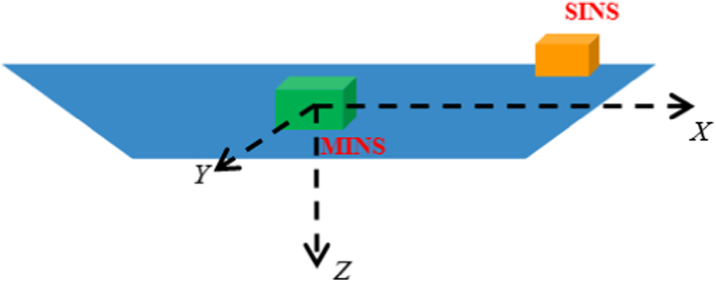
The problems that need to be considered in terms of transfer alignment include the lever-arm effect, ship flexure, mounting misalignment and time delay as shown in Figure 1. The effects of lever-arm effect and ship flexure confine the alignment accuracy and rapidity in the presence of the ship dynamics, which are difficult to compensate for due to their uncertainties. The lever-arm effect is caused by the relative distance between the MINS and the SINS. Since the ship flexure is difficult to accurately model due to the error that is caused by the bending of the ship, it is generally applied to the nonlinear filter for the transfer alignment through the assumption of a second-order Markov model. The time delay does not have much of an effect in the stationary state, but the time difference between the MINS and the SINS causes an error when the ship is at sea. The mounting misalignment between the MINS and the SINS causes a large error if it is not compensated.
Figure 1. The structure of the transfer alignment process.
2.1. Lever-arm effect
In transfer alignment, the lever arm effect means that relative velocity and acceleration occurs due to the relative distance between SINS and MINS, as shown in Figure 2. Therefore, since transfer alignment aligns the SINS by using information from the MINS, the lever-arm effect should be considered (Joon and You-Chol, Reference Joon and You-Chol2009). If the ship is a rigid body, the lever arm effect affects velocity and acceleration, and this is considered for the performance of velocity acceleration matching. The relationship between the relative velocity and the angular velocity is as follows:

Figure 2. Relative position of the SINS to the MINS.
 $$V_S^n=V_M^n+C_M^n(\omega_{nM}^{M}\times r_0)$$
where  $V_{S}^{n}$ is the SINS velocity,
  $V_{M}^{n}$ is the MINS velocity,
  $\omega_{nM}^{M}$ is the MINS angular velocity,
  $C_{M}^{n}$ is the MINS body-to-navigation frame direction cosine matrix and r 0 is the fixed lever-arm vector without considering ship flexure.
2.2. Ship flexure
Ship flexure is generally applied to nonlinear filters for transfer alignment, assuming a second-order Markov model. This is because it is difficult to model ship flexure due to the error caused by the bending of the ship (Joon and You-Chol, Reference Joon and You-Chol2009). It is assumed that the flexure angle changes due to ship flexure as follows:
 $$\begin{align} &\ddot{\theta}+\alpha\dot{\theta}+\beta\theta=\eta\\ &\alpha=2\zeta w_n,\quad \beta=w_n^2,\quad \eta\sim N(0,\sigma^2) \end{align}$$
where θ is the flexure angle  $\dot{\theta}$,
  $\ddot{\theta}$ are angular velocity and angular acceleration of the flexure angle and
  $\zeta, w_{n},\sigma$ are parameters of the Markov model.
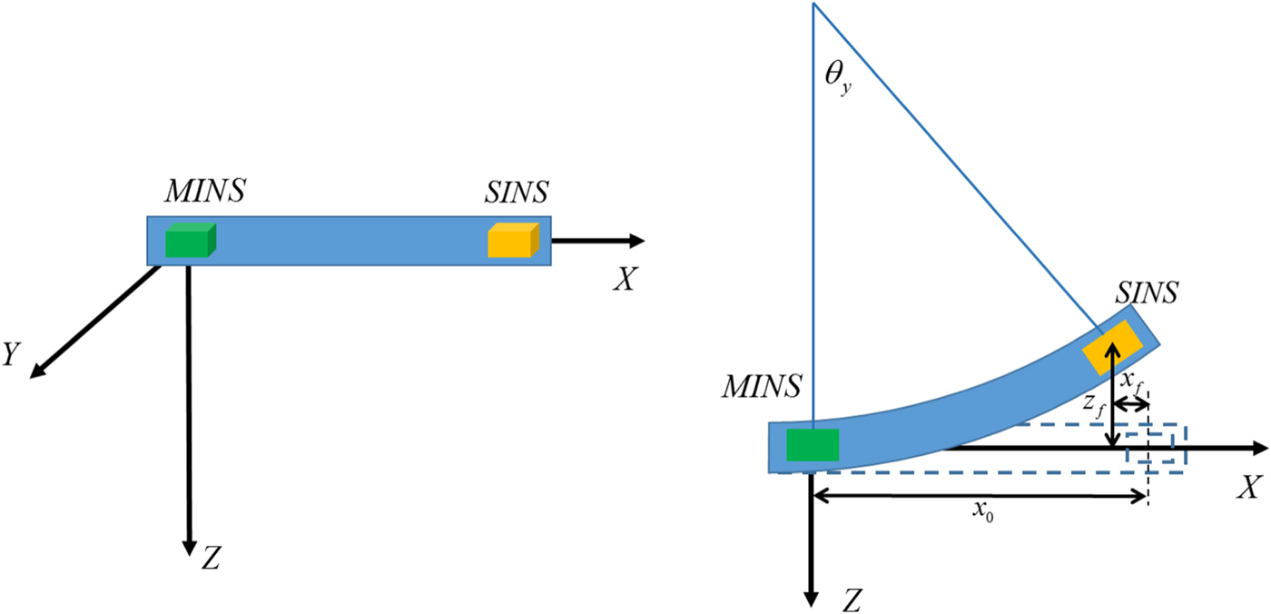
The lever-arm variations are caused by the flexure angle, as shown in Figure 3; this relationship allows us to calculate the changed lever-arm vector according to the flexure angle. First, the changed value of the lever-arm vector due to the y-axis flexure angle of the ship is expressed as follows:
 $$\begin{align} z_f&=x_0\frac{1-\cos\theta_y}{\theta_y}=x_0\frac{2\sin^2\frac{\theta_y}{2}}{\theta_y}\label{eq3} \end{align}$$
 $$\begin{align} x_f&=-x_0\left(1-\frac{\sin \theta_y}{\theta_y}\right)\label{eq4} \end{align}$$
Assuming that θ y is a small angle, it can be simplified as follows:
 $$\begin{align} & z_f\ \widetilde{=}\ x_0\frac{\theta_y}{2}\label{eq5} \end{align}$$
 $$\begin{align} & x_f\ \widetilde{=}\ 0\label{eq6} \end{align}$$
Therefore, if the other axes are calculated, the lever-arm vector for the ship flexure is as follows:
 $$\begin{align}r=\left[\begin{matrix} x_0+\dfrac{\theta_y}{2}z_0-\dfrac{\theta_z}{2}y_0 \\\noalign{\vskip6pt} y_0+\dfrac{\theta_z}{2}x_0-\dfrac{\theta_x}{2}z_0 \\\noalign{\vskip6pt} z_0+\dfrac{\theta_x}{2}y_0-\dfrac{\theta_y}{2}x_0 \end{matrix}\right]=r_0-\left(\frac{1}{2}r_0\times\right)\theta \end{align}$$
where  $r_{0}=\left[\begin{smallmatrix}x_{0}& y_{0}& z_{0}\end{smallmatrix}\right]^{T}$ and
  $\theta=\left[\begin{smallmatrix}\theta_{x}& \theta_{y}& \theta_{z}\end{smallmatrix}\right]^{T}$.

Figure 3. Relationship between the y-axis flexure angle and the lever-arm vector.
2.3 Transfer-alignment system model
Regarding the model for the design of the Extended Kalman Filter (EKF) for which the ship flexure, mounting misalignment and time delay are considered, the 19 error states are expressed as follows:
 $$\delta x=\left[\begin{matrix}\delta V^n& \varphi^n&\nabla^S&\varepsilon^S& \delta\theta^M&\delta\dot{\theta}^M&\delta t_{delay} \end{matrix}\right]^T$$
where the velocity errors (δ V n), attitude errors (φn), accelerometer bias (∇S), gyro biases  $(\varepsilon^{S})$ of the SINS and the flexure angle errors
  $(\delta\theta^{M})$, flexure angular velocity errors
  $(\delta\dot{\theta}^{M})$, and time delay errors
  $(\delta t_{delay})$ are contained.
Since the flexure angle and the flexure angular velocity follow the second-order Markov model, a corresponding system-error model should be established as follows:
 $$\begin{align}\label{eq9} \delta\dot{x}(t)&=F(t)\delta x(t)+w(t),\ w(t)\sim N(0,Q)\nonumber\\ &=\left[\begin{matrix} F_{vv}& F_{v\varphi}& F_{v\nabla}&0_{3\times 3}&0_{3\times 3}&0_{3\times 3}&0_{3\times 1}\\ F_{\varphi v}& F_{\varphi\varphi}&0_{3\times 3}& F_{\varphi\varepsilon}&0_{3\times 3}&0_{3\times 3}&0_{3\times 1}\\ 0_{6\times 3}&0_{6\times 3}&0_{6\times 3}&0_{6\times 3}&0_{6\times 3}&0_{6\times 3}&0_{6\times 1}\\ 0_{3\times 3}&0_{3\times 3}&0_{3\times 3}&0_{3\times 3}&0_{3\times 3}& F_{\theta\dot{\theta}}&0_{3\times 1}\\ 0_{3\times 3}&0_{3\times 3}&0_{3\times 3}&0_{3\times 3}& F_{\dot{\theta}\theta}& F_{\dot{\theta}\dot{\theta}}&0_{3\times 1}\\ 0_{1\times 3}&0_{1\times 3}&0_{1\times 3}&0_{1\times 3}&0_{1\times 3}&0_{1\times 3}&0_{1\times 1}\\ \end{matrix}\right]\delta x(t)+\left[\begin{matrix}w_a(t)\\ w_g(t)\\ 0_{10\times1}\\ \sigma(t)\end{matrix}\right] \end{align}$$
where w a is the velocity random walk of the SINS and w g is the angular random walk of the SINS.
 $$\begin{align}F_{vv}&=\left[\begin{matrix} v_D/(R_m+h)&2\Omega_D+2\rho_D&\rho_E\\ -2\Omega_D-\rho_D&(v_N\tan L+v_D)/(R_t+h)&2\Omega_N+\rho_N\\ 2\rho_E&-2\Omega_N-3\rho_N&0 \end{matrix}\right],\\ F_{v\varphi}&=\left[\begin{matrix} 0&-f_D& f_E\\ f_D&0&-f_N\\ -f_E& f_N&0 \end{matrix}\right]=(C_b^nf^b)\times F_{\varphi v}=\left[\begin{matrix} 0&1/(R_t+h)&0\\ -1/(R_m+h)&0&0\\ 0&-\tan L/(R_t+h)&0 \end{matrix}\right], \\ F_{\varphi\varphi}&=\left[\begin{matrix} 0&\Omega_D+\rho_D&-\rho_E\\ -\Omega_D-\rho_D&0&\Omega_N+\rho_N\\ \rho_E&-\Omega_N-\rho_N&0 \end{matrix}\right]\\ F_{\theta\dot{\theta}}&=I_{3\times3},\ F_{\dot{\theta}\theta}=- \left[\begin{matrix} 0&-\alpha_z&\alpha_y\\ \alpha_z&0&-\alpha_x\\ -\alpha_y&\alpha_x&0 \end{matrix}\right],\ F_{\dot{\theta}\dot{\theta}}=-\left[\begin{matrix} 0&-\beta_z&\beta_y\\ \beta_z&0&-\beta_x\\ -\beta_y&\beta_x&0 \end{matrix}\right]\end{align}$$
F vv, F vφ, F φ v and  $F_{\varphi\varphi}$ are well-known values in inertial navigation systems and readers are referred to Titterton and Weston (Reference Titterton and Weston2004).
  $F_{\theta\dot{\theta}}$ and
  $F_{\theta\dot{\theta}}$ are the values associated with flexure.
3. MATCHING METHODS
Transfer alignment in real environments should be able to estimate sensor turn-on biases as well as velocity and attitude solutions with consideration of the several environmental parameters mentioned in the previous section. However, it may be difficult to estimate the sensor biases accurately when sufficient alignment time is not permitted. It is assumed that the velocity and attitude measurements are used, and this is the calculated parameter matching method. It is well known that this method is observable. However, fast estimation of the sensor biases is not provided in rapid alignment. To increase the alignment speed, the angular velocity measurement can be additionally used. That is the measured parameter matching method. One more measured parameter – acceleration – can be considered as another measurement to include. To consider the lever-arm effect, angular acceleration information is essential when the acceleration measurement is adopted, however, this information can be obtained by numerical differentiation of the angular velocity measurement. Therefore, the effectiveness of the acceleration matching depends on the MINS angular random walk, SINS velocity random walk and lever-arm length. In this respect, the effectiveness of the acceleration matching method must be analysed in terms of the estimation accuracy and alignment speed. In this section, several measurement equations are designed according matching measurements.
3.1. Velocity matching
The measurement equation for the velocity matching method for which the ship flexure is considered, as defined in Section 2.2, can be expressed as follows:
 $$\begin{align}z_v=\hat{V}_S^n-(V_M^n+C_M^n(\omega_{nM}^{M}\times\hat{r}+\hat{\dot{r}})),\ r=r_0-\left(\frac{1}{2}r_0\times\right)\theta,\ \dot{r}=-\left(\frac{1}{2}r_0\times\right)\dot{\theta}\end{align}$$
The measurement equation can be expanded as following equation for generating an error equation that will be used in the EKF as follows:
 $$\begin{align} z_v&=\delta V_S^n-\delta V_M^n-C_M^n(\omega_{nM}^M\times \delta r+\delta \dot{r})+ \left(\frac{V_{S,k-1}^n-V_S^n}{dt}\right)\delta t_{delay}\nonumber\\ &=\delta V_S^n-\delta V_M^n-C_M^n\left(\omega_{nM}^M\times\left(-\left(\frac{1}{2}r_0\times\right) \delta\theta\right)+\left(-\left(\frac{1}{2}r_0\times\right)\delta\dot{\theta}\right)\right)\nonumber\\ &\quad +\left(\frac{V_{S,k-1}^n-V_S^n}{dt}\right)\delta t_{delay}\label{eq11} \end{align}$$
This is represented by the measurement matrix as follows:
 $$\begin{align}\label{eq12} z_v&=H\delta x+v=[ \vphantom{( \dfrac{V_{S,k-1}^n-V_S^n}{dt}) ( -\dfrac{r_0}{2}\times) }I_{3\times3}\quad 0_{3\times3}\quad 0_{3\times3}\quad 0_{3\times3}\quad -C_M^n(\omega_{nM^M}\times)( -\dfrac{r_0}{2}\times) \nonumber\\ &\quad -C_M^n( -\dfrac{r_0}{2}\times) \quad ( \dfrac{V_{S,k-1}^n-V_S^n}{dt}) ] \delta x+v, \end{align}$$
where  $v\sim N(0,R_{V_{M}})$ is the MINS velocity noise.
3.2. Attitude matching
The attitude matching is performed in a Direction Cosine Matrix (DCM) matching form, considering flexure angle as follows:
 $$\begin{align} Z_{\varphi}&=C_{M}^n\hat{C}_{M'}^{M}C_{S}^{M'}\hat{C}_{n}^{S}-I_{3\times 3}\label{eq13} \end{align}$$
 $$\begin{align} Z_{\varphi}&=C_{M}^n(I_{3\times 3}-(\delta\theta\times))C_{M'}^{M} C_{S}^{M'}(I_{3\times 3}+(\omega_{nS}^S\times)\delta t_{delay}) C_n^S(I_{3\times 3}+(\varphi\times))-I_{3\times 3}\nonumber\\ &\approx(\varphi\times)-C_M^n(\delta\theta\times)+C_S^n(\omega_{nS}^S\times)\delta t_{delay}\label{eq14} \end{align}$$
where  $w_{nS}^{S}$ is the SINS angular velocity,
  $C_{S}^{M'}$ is the DCM of the known attitude between the MINS and the SINS and
  $C_{M'}^{M}$ is the DCM of the flexure angle. Since the values on the right-hand side are all skew-symmetric matrix types, the following equation can be defined:
 $$z_{\varphi}=\left(\begin{matrix}-Z_{\varphi} (2,3)\\\noalign{\vskip4pt} Z_{\varphi} (1,3)\\\noalign{\vskip4pt} -Z_{\varphi} (1,2)\end{matrix}\right)= \varphi-C_M^n\delta\theta+C_S^n\omega_{nS}^S\delta t_{delay}+v\label{eq15}$$
 $$z_{\varphi}=H\delta x+v=\left[\begin{matrix}0_{3\times3}& I_{3\times3}&0_{3\times3}&0_{3\times3}&-C_M^n&0_{3\times3}& C_S^n\omega_{nS}^S\end{matrix}\right]\delta x+v$$
where  $v\sim N(0,R_{\varphi_{M}})$ is the MINS attitude noise.
3.3. Angular-velocity matching
If the angular-velocity information of the MINS can be utilised, a measurement model can be constructed with the use of the SINS and MINS angular velocities as follows:
 $$\begin{align} z_{\omega}&=\omega_{nS}^{S}-\hat{C}_{M'}^{S}\hat{C}_{M}^{M'} (\omega_{nM}^{M}-\hat{\dot{\theta}})\label{eq17} \end{align}$$
 $$\begin{align} z_{\omega}&=C_{M'}^{S}(C_{M}^{M'}(\omega_{nM}^M-\dot{\theta}))\times\delta\theta+ C_{M'}^{S}C_{M}^{M'}\delta\dot{\theta}+\left(\frac{\omega_{nS,k-1}^S-\omega_{nS,k}^{S}}{dt}\right)\delta t_{delay}+v\label{eq18} \end{align}$$
 $$\begin{align} z_{\omega}&=H\delta x+v=[ 0_{3\times3}\quad 0_{3\times3}\quad 0_{3\times3}\quad I_{3\times3}\quad C_{M'}^{S}(C_{M}^{M'}(\omega_{nM}^M-\dot{\theta})) \nonumber\\ &\quad\times\left. C_{M'}^{S}C_{M}^{M'}\quad\left(\frac{\omega_{nS,k-1}^S-\omega_{nS,k}^{S}}{dt}\right)\right]\delta x+v\label{eq19} \end{align}$$
where  $v\sim N(0,R_{\omega})$,
  $R_{\omega}=(\gamma_{SINS})^{2}+(\gamma_{MINS})^{2}$, for which γSINS is the white noise of the SINS gyroscope signal and γMINS is the white noise of the MINS gyroscope signal.
3.4. Acceleration matching
If the MINS measured acceleration can be utilised, a measurement model can be constructed as follows:
 $$\begin{align} z_{f}&=f^S-\hat{C}_{M'}^S\hat{C}_{M}^{M'}(f^M+\omega_{nM}^M\times \omega_{nM}^M\times \hat{r} +2\omega_{nM}^{M}\times \hat{\dot{r}}+\alpha_{nM}^M\times\hat{r}+\ddot{r})\label{eq20} \end{align}$$
 $$\begin{align} z_{f}&=\delta f^{S}+\left(\frac{f_{k-1}^{S}-f_k^S}{dt}\right)\delta t_{delay}+C_{M'}^S\nonumber\\ &\quad \times( C^{M'}_M(f^M+\omega_{nM}^{M}\times\omega_{nM}^{M}\times r+2\omega_{nM}^{M} \dot{r}+\alpha_{nM}^M\times r)) \times \delta\theta\nonumber\\ &\quad -C_{M'}^SC^{M'}_M((\delta f^{M}+\omega_{nM}^{M}\times \omega_{nM}^{M}\times \delta r+2\omega_{nM}^{M}\times \delta\dot{r}+\alpha_{nM}^{M}\times\delta r+r\times\delta\alpha_{nM}^M\nonumber\\ &\quad -(\omega_{nM}^{M}\times r\times + (\omega_{nM}^{M}\times r)\times+2\dot{r}\times)\delta\omega_{nM}^{M}))\label{eq21} \end{align}$$
where f M and f S are the MINS and SINS accelerations, respectively, and  $\alpha_{nM}^{M}$ is the MINS angular acceleration that is obtained from the numerical differentiation of the measured MINS angular velocity. This is represented by the measurement matrix as follows:
 $$\begin{align} z_f&=H\delta x+v,v\sim N(0,R_f)\\ z_f&=H\delta x+v=[0_{3\times 3}\quad 0_{3\times 3}\quad I_{3\times 3}\quad 0_{3\times 3}\quad H_{\theta}\quad H_{\dot{\theta}}\quad H_{\delta t_{delay}}]\delta x+v \end{align}$$
where the following formulae apply:
 $$\begin{align}{H_{\theta}&=( C_{M'}^{S}( C_{M'}^{M}( f^{M}+\omega_{nM}^{M}\times \omega_{nM}^{M}\times r+2\omega_{nM}^{M}\times \dot{r}+\alpha_{nM}^{M}\times r) ) \times) \\ &\quad +C_{M'}^{S}\ C_{M}^{M'}( \omega_{nM}^{M}\times\omega_{nM}^{M}\times +\alpha_{nM}^{M}\times) \left(\frac{1}{2}r_{0}\times\right),\\ H_{\dot{\theta}}&=C_{M'}^{S}\ C_{M}^{M'}( 2\omega_{nM}^{M}\times) \left(\frac{1}{2}r_{0}\times\right),\quad H_{\delta t_{delay}}=\left(\frac{f_{k-1}^{S}-f_{k}^{S}}{dt}\right), \quad \nu\sim N(0,R_{f})}\end{align}$$
The effectiveness of the acceleration matching is determined according to R f, which contains various error factors. Detailed R f is discussed in Section 4.2. It is difficult to yield analytical results to evaluate the effectiveness of the acceleration matching. In this paper, therefore, simulation results are presented under the various error factors.
4. SIMULATION RESULTS
To analyse the acceleration matching, simulation of the transfer alignment is implemented in consideration of the lever-arm effect, ship flexure and time delay. In this simulation, we focus on the major factors that have a significant impact on the performance of the transfer alignment using accelerated matching. In the rapid alignment, the alignment performance is less affected by motion; therefore, this simulation deals with constant velocity motion, which varies slightly due to waves (Joon and You-Chol, Reference Joon and You-Chol2009).
4.1. Performance difference by matching methods
Ship flexure is modelled according to the Markov process with the ship-flexure parameter, as shown in Table 1 (Joon and You-Chol, Reference Joon and You-Chol2009). The simulation conditions are specified in Tables 2 to 4. The SINS and MINS error elements are taken into consideration for the actual sensor performance.
Table 1. Ship-flexure parameters

Table 2. Simulation environments
Table 3. SINS error elements.

Table 4. MINS error elements.
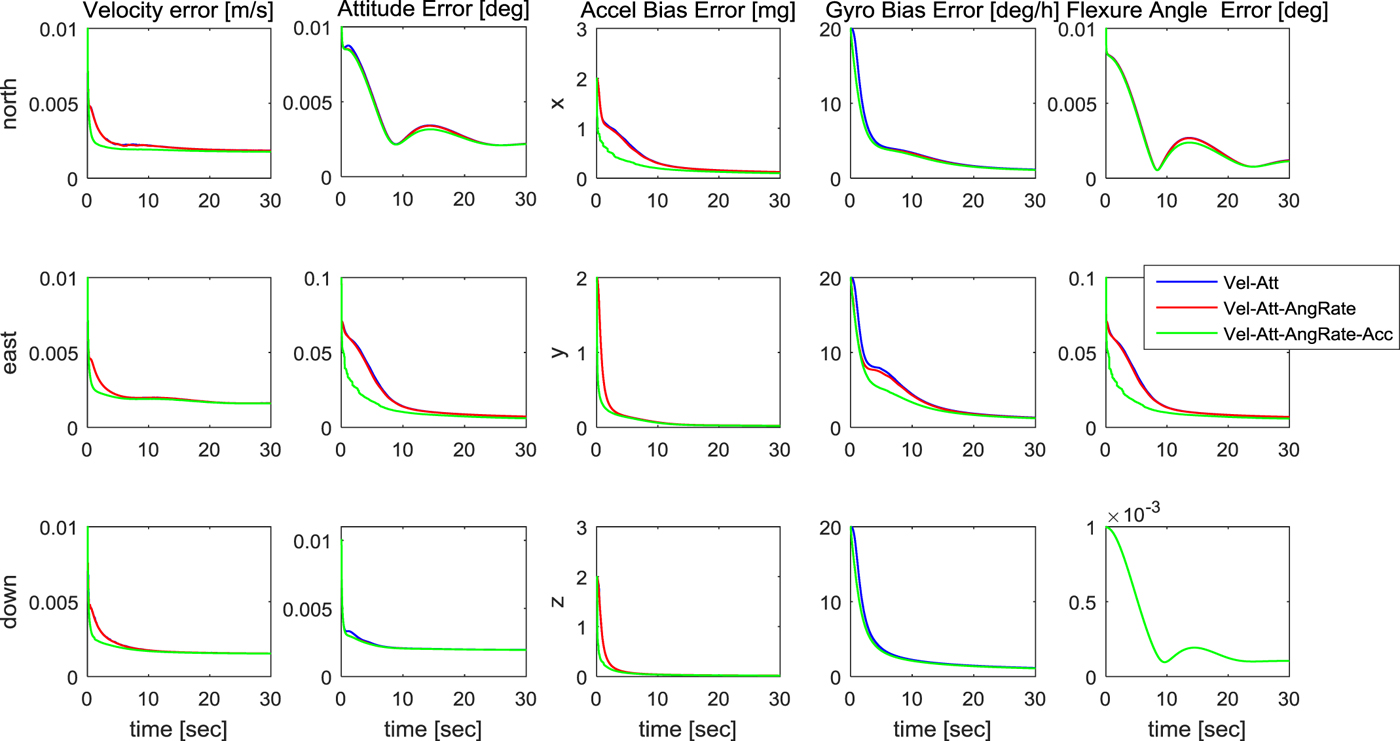
The convergence speed of the error standard deviation by matching methods is shown in Figure 4. Each panel shows error standard deviation of the velocity, attitude, accelerometer bias, gyro bias and flexure angle, respectively. Each panel in the longitudinal direction represents the error covariance of each axis. Velocity and attitude error are shown on the north, east, down axes, and accelerometer bias, gyro bias, flexure angle error are shown on the x, y, z axes. Figure 5 shows the convergence speed of the time delay error standard deviation by matching methods. When angular rate matching is added to velocity and attitude matching, a large convergence speed improvement is not shown. However, when acceleration matching is added to velocity, attitude and angular rate matching, the convergence speed noticeably increases. As shown in Equation (22), in the case of acceleration matching, the acceleration measurements have a direct effect on the estimation of the acceleration bias, flexure angle and time delay. Therefore, the directly affected states are estimated quickly. Especially, the y-axis flexure angle can be estimated quickly during acceleration matching because the flexure angle in the y-axis direction of the ship is larger than the other axes. When all of the four matching measurements are used, the acceleration matching method also has an effect on the performance of other matching methods. First, the attitude error of the y-axis is quickly estimated due to the fast estimation of the y-axis flexure angle during the attitude matching. In addition, the x-axis accelerometer bias ∇X is also estimated quickly by the velocity matching. This can be confirmed through the following velocity error model:

Figure 4. Error standard deviation convergence speed by matching methods.
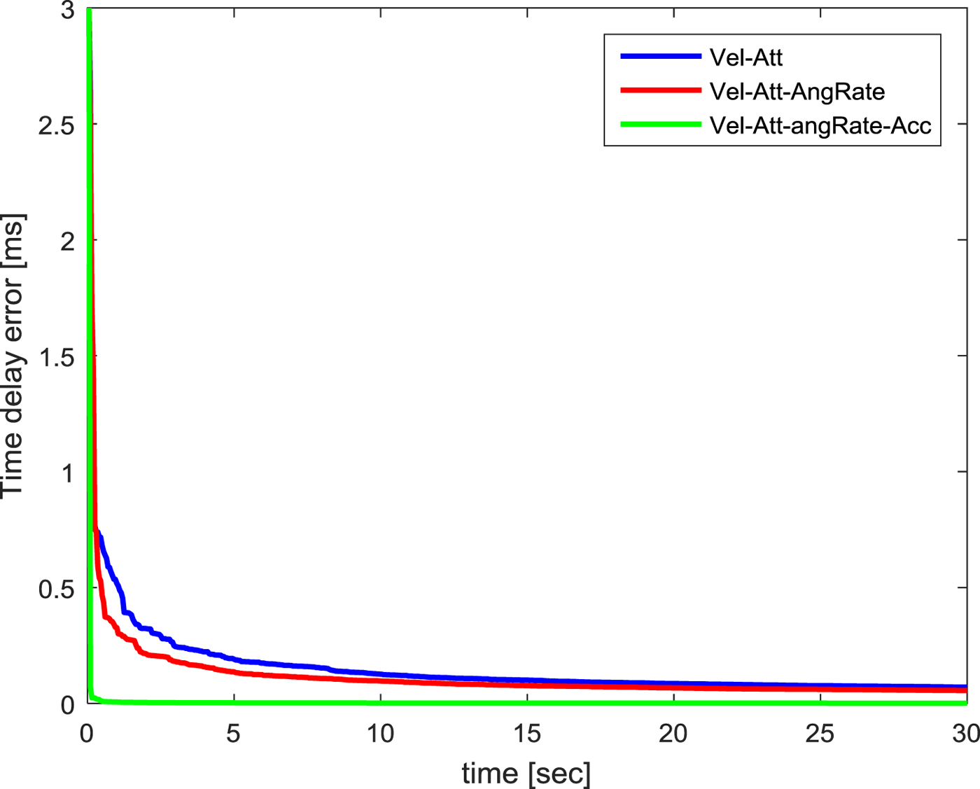
Figure 5. Convergence speed of time delay error standard deviation by matching methods.
 $$\begin{align}\label{eq23} \delta\dot{V}&=F_{\nu\nu} V^{n}+F_{v\varphi}\varphi^{n}+F_{\nu\nabla}\nabla^{S}\nonumber\\ &=F_{\nu\nu}\left[\begin{matrix}\delta \nu_{N}\\ \delta \nu_{E}\\ \delta \nu_{D}\end{matrix}\right]+( C_{b}^{n}\ f^{b}) \times \left[\begin{matrix}\phi_{N}\\ \phi_{E}\\ \phi_{D}\end{matrix}\right]+C_{b}^{n}\left[\begin{matrix}\nabla_{X}\\ \nabla_{Y}\\ \nabla_{Z}\end{matrix}\right] \end{align}$$
where  $F_{\nu\nu},F_{\nu\varphi},F_{\nu\nabla}$ are as mentioned in Equation (9). The result obtained by multiplying
  $C_{n}^{b}$ by both sides and using the properties of a skew symmetric matrix are as follows:
 $$\begin{align}\label{eq24} C_{n}^{b} \delta\dot{V}^{n}&=C_{n}^{b} F_{\nu\nu}\left[\begin{matrix}\delta \nu_{N}\\ \delta \nu_{E}\\ \delta \nu_{D}\end{matrix}\right]+C_{n}^{b}( ( C_{b}^{n}\ f^{b}) \times) C_{n}^{b}\left[\begin{matrix}\phi_{X}\\ \phi_{Y}\\ \phi_{Z}\end{matrix}\right]+C_{n}^{b} C_{b}^{n}\left[\begin{matrix}\nabla_{X}\\ \nabla_{Y}\\ \nabla_{Z}\end{matrix}\right]\nonumber\\ &=C_{n}^{b} F_{\nu\nu}\left[\begin{matrix}\delta \nu_{N}\\ \delta \nu_{E}\\ \delta \nu_{D}\end{matrix}\right]+\begin{bmatrix}0&-f_{Z}& f_{X}\\ f_{Z}& 0 & -f_{Y}\\ -f_{Y}& f_{X} & 0\end{bmatrix}\left[\begin{matrix}\phi_{X}\\ \phi_{Y}\\ \phi_{Z}\end{matrix}\right]+\left[\begin{matrix}\nabla_{X}\\ \nabla_{Y}\\ \nabla_{Z}\end{matrix}\right] \end{align}$$
Generally, the z-axis acceleration f Z including gravity has a larger value than f X and f Y. In the first line of the velocity error model, the y-axis attitude error ϕ Y is multiplied by f Z, which has a large value. Therefore, the smaller ϕ Y is, the faster estimation of the acceleration ∇X bias. In other words, the largest y-axis flexure angle is rapidly estimated during acceleration matching, and ϕ Y and ∇X are estimated quickly by attitude and velocity matching. This relationship is also shown in Figures 4 and 5. Therefore, acceleration matching helps improve the error state estimation speed. In this paper, we use the x-axis acceleration bias as the performance criterion, which has a remarkably improved estimation speed.
4.2. Analysis of performance improvement by acceleration matching
As mentioned previously, acceleration matching can be effective depending on the performance of the MINS angular random walk, the SINS velocity random walk, the lever-arm length and the alignment time. To indicate the performance of acceleration matching, the performance index is set as follows:
 $$E_{AM}=\sqrt{P_{\nabla_{X}}}-\sqrt{P_{\nabla_{X},acceleration matching}}$$
where E AM is the performance index of the acceleration matching and  $P_{\nabla_{X},acceleration matching}$ and
  $P_{\nabla_{X}}$ are the error covariance of the x-axis accelerometer bias. Both values are the results of performance velocity, attitude and angular rate matching with the difference being due to whether acceleration matching is performed or not. E AM shows by how much the estimation error of the x-axis acceleration bias is reduced by the acceleration matching. As mentioned in Section 4.1, in the case of a ship, in general with a long shape along the x-axis, the y-axis attitude error may be large due to ship flexure. Therefore, the y-axis flexure angle can be quickly estimated when acceleration matching is adopted. Consequently, the y-axis attitude error and the associated x-axis accelerometer bias can also be estimated quickly. Therefore, in this study, E AM is used as the performance evaluation criterion of the acceleration matching method.
E AM according to alignment time is shown in Figure 6. Acceleration matching has a profound effect when the alignment time is short. Since there are many factors affecting the transfer alignment performance according to the acceleration matching, we show the result that the alignment time is fixed to one second and the transfer alignment performance according to several factors is analysed in the rapid transfer alignment with the fixed alignment time. The effectiveness of the acceleration matching is determined according to R f, which is the measurement noise, as follows:
 $$R_{f}=( \delta a^{S}) ^{2}+ A( \delta w_{nM}^{M}) ^{2}\ A^{T}+B( \delta\alpha_{nM}^{M}) ^{2} B^{T}+C( \alpha a^{M}) ^{2} C^{T}$$
 $$A=C_{M'}^{S} C_{M}^{M'}( \omega_{nM}^{M}\times r \times +( \omega_{nM}^{M}\times r) \times +2\dot{r}\times ),\quad B=C_{M}^{S},C_{M}^{M'}r\times,\quad C=C_{M'}^{S}\ C_{M}^{M'}$$
where δ a S is the SINS-accelerometer white noise,  $\delta\omega_{nM}^{M}$ is the MINS-gyro white noise,
  $\delta\alpha_{nM}^{M}$ is the MINS white noise of the angular acceleration and δ a M is the MINS-accelerometer white noise. Since
  $\delta\alpha_{nM}^{M}$ is obtained by numerical differentiation of the measured angular velocity
  $\delta\omega_{nM}^{M},\delta\alpha_{nM}^{M}$ has a much greater white noise than
  $\delta\omega_{nM}^{M}\cdot \delta\alpha_{nM}^{M}$ can be expressed as the numerical derivative of
  $\delta\omega_{nM}^{M}$, as follows:
 $$\delta\alpha_{nM}^{M}=\frac{\sqrt{2}}{dt}\delta\omega_{nM}^{M}$$
where dt is the sampling rate of the sensors. In addition, δ a S is generally much larger than δ a M; so the effects of  $\delta\omega_{nM}^{M}$ and δ a M are negligible, and
  $\delta\alpha_{nM}^{M}$ and δ a S largely influence the effectiveness of the acceleration matching. The lever-arm length, r, is also important because it is tied to
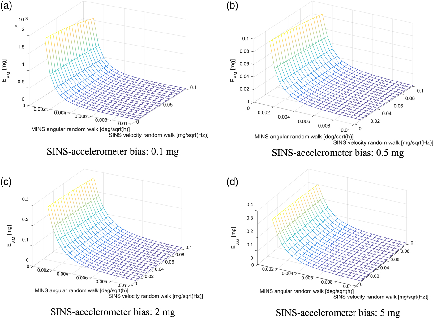
  $\delta\alpha_{nM}^{M}$. To analyse the effect on these values, various simulations were carried out by changing the values in Table 5. As shown in Figure 7, when the lever-arm length is large,
  $\delta\omega_{nM}^{M}$ is more important than δ a S in the acceleration-matching performance. As shown in Figure 7, there is no performance difference for δa S when the lever-arm is large. Comparing Figure 7(a) with 7(d), the larger the initial acceleration bias is, the greater the effect of acceleration matching, but the above tendency does not change significantly.
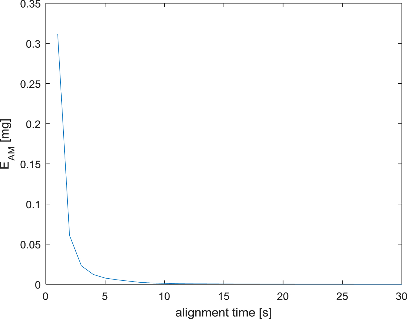
Figure 6. Performance index according to the alignment time.

Figure 7. Performance index according to the various elements (lever-arm vector: [50,0,0] m).
Table 5. Various elements affecting the acceleration-matching performance.

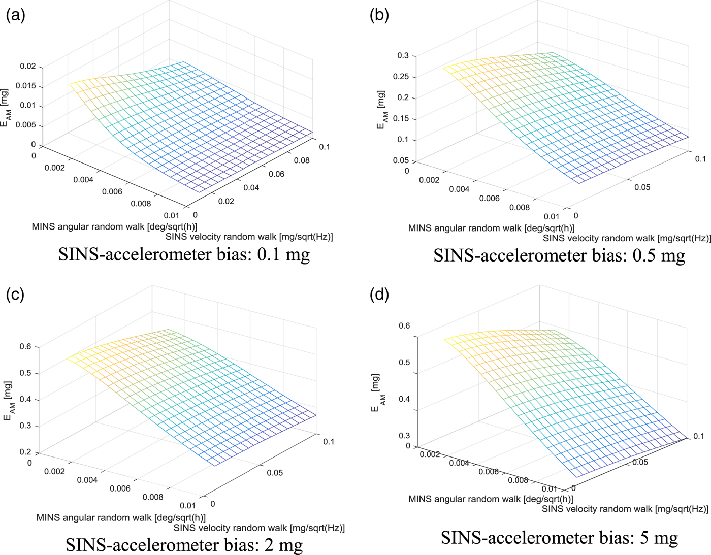
If the lever-arm length is small, δ a S is also important for acceleration-matching performance, as shown in Figure 8. The smaller  $\delta\omega_{nM}^{M}$ is, the clearer the performance improvement by δ a S is. Comparing Figures 8(a) and 8(d), the larger the initial acceleration bias, the greater the effect of acceleration matching. The effect of acceleration matching on δ a s and δ a S varies depending on the initial acceleration bias as shown in Figure 8. In addition, by comparing Figures 7 and 8, it can be confirmed that the transfer alignment performance is better when the lever-arm length is short. As mentioned above, acceleration matching can be effective depending on the performances of the MINS angular random walk, the SINS velocity random walk, the lever-arm length, and the alignment time. The repeatability of the SINS-accelerometer bias is also relevant. Depending on the lever-arm length, the effect of changes in δ a S on the effectiveness of acceleration matching is different, the results of which are summarised in Table 6.

Figure 8. Performance index according to the various elements (lever-arm vector: [5,0,0] m).
Table 6. Conditions that increase the effectiveness of acceleration matching.

5. CONCLUSION
This research is based on the velocity, attitude, angular velocity and acceleration matching methods of transfer alignment. In general, acceleration matching is considered as unworkable for transfer alignment, but acceleration matching can be effective depending on the performance of the MINS angular random walk, the SINS velocity random walk, the lever-arm length and the alignment time. To analyse the acceleration matching performance, a transfer-alignment simulation was implemented in consideration of the lever-arm effect, ship flexure and time delay. In this paper, the focus is the effectiveness of acceleration matching according to sensor performance during rapid transfer alignment. Performance analysis of the simulation results using the performance index showed the validity of the acceleration matching according to the MINS angular velocity random walk, the SINS velocity random walk, SINS accelerometer bias and the lever-arm length.
ACKNOWLEDGMENTS
This work was supported by Agency for Defense Development [UD150004DD].