2. Experimental methodology

2.1. Experimental set-up

Experiments were performed in the water tunnel of the Institute of Fluid Mechanics at the Beijing University of Aeronautics and Astronautics, which has a test section of 600 × 600 × 3000 mm (height × width × length). The free stream turbulence intensities were no more than 0.8 % for all the test cases. The current 30P30N multi-element airfoil is a scaled model of AIAA BANC-II Workshop (Choudhari & Lockard Reference Choudhari and Lockard2015). It has a stowed chord length (c) of 150 mm and an aspect ratio of 3.33. The slat has a chord length (c_s = 15 %c) of 22.5 mm. The aspect ratio (Jenkins et al. Reference Jenkins, Khorrami and Choudhari2004; Pascioni & Cattafesta Reference Pascioni and Cattafesta2018b) and the circular endplates at two sides of the airfoil (Boutilier & Yarusevych Reference Boutilier and Yarusevych2012) guarantee a quasi-two-dimensional mean flow around the mid-span region of the airfoil (Wang et al. Reference Wang, Wang and Kim2019). Therefore, the wall effects on the flow physics discussed in the current work were negligible. No boundary layer trip was used. The geometric angle of attack, defined as the angle between the chord line of the clean configuration and the inflow direction, was fixed at 4 °. Notably, the high camber and the strong circulation of the multi-element airfoil induced high-flow deflection, which led to evident deviations between the geometric and the effective angles of attack in the measurement with an open-jet wind tunnel (Murayama et al. Reference Murayama, Nakakita, Yamamoto, Ura, Ito and Choudhari2014; Manoha & Pott-Pollenske Reference Manoha and Pott-Pollenske2015; Li et al. Reference Li, Liu, Guo, Hou, Geng and Wang2017; Jawahar et al. Reference Jawahar, Ali, Azarpeyvand and da Silva2020). Normally, the geometric angle of attack is shifted to an effective angle of attack according to the pressure distributions above the multi-element airfoil (Murayama et al. Reference Murayama, Nakakita, Yamamoto, Ura, Ito and Choudhari2014; Pascioni & Cattafesta Reference Pascioni and Cattafesta2018b; Jawahar et al. Reference Jawahar, Ali, Azarpeyvand and da Silva2020). Because the current experimental set-up was designed to be focused on the evolutions of flow structures in a water tunnel, the pressure distributions above the multi-element airfoil were unavailable and therefore no aerodynamic correction was applied to the current results. Accordingly, an effective angle of attack was unavailable in the current work. Li et al. (Reference Li, Liu, Guo, Hou, Geng and Wang2017) has shown that the pressure distribution and flow field of a 30P30N configuration in a closed hard-wall wind tunnel are comparable to those in ideal free flight conditions. Therefore, the deviations between the geometric and the effective angles of attack of the multi-element airfoil are alleviated in the measurement with a closed hard-wall wind tunnel. The current experiments were performed in a water tunnel, comparable to those performed in a closed hard-wall wind tunnel. Therefore, it could be deduced that the current effective angle of attack was still approximately 4 °. The origin of the coordinate system (O in figure 1) was located at the leading edge of the slat at α = 0 °, consistent with Wang et al. (Reference Wang, Feng, Wang and Li2018, Reference Wang, Wang and Kim2019). X and Y denote the streamwise and vertical directions, respectively. As the free stream velocity U_∞ varied from 62 to 348 mm s⁻¹, the Reynolds number based on c (Re_c) varied from 9.3 × 10³ to 5.2 × 10⁴. More details of the model design and related water tunnel can be found in the papers by Wang et al. (Reference Wang, Feng, Wang and Li2018, Reference Wang, Wang and Kim2019).

Figure 1. Experimental set-up. The distances between the lasers and the airfoil are longer than those sketched in (a). The field of view of TR-PIV measurements is sketched by the black box in (b).

Two-dimensional TR-PIV was used to measure the flow around the slat cove. The flow was seeded with hollow glass beads with a median diameter of 10 μm. Two semiconductor continuous lasers (8 W, 532 nm) were co-operated to illuminate the gap region between the slat and the main element, by aligning the two laser sheets (thickness of ~1 mm) to one plane (figure 1a). PIV images were captured by a Photron FASTCAM SA2 high-speed CMOS camera with a TAMRON lens (focal length of 90 mm). The field of view was fixed as 23 mm × 32 mm (sketched by a black box in figure 1(b)). The shutter time of the CMOS camera equalled 1/f_s, where f_s is the sampling frequency of the CMOS camera. An increase of Re_c from 9.3 × 10³ to 5.2 × 10⁴ led to an increase of f_s from 250 to 1500 Hz. The magnification was fixed as 0.035 mm pix⁻¹. The velocity fields were calculated by the multi-pass iterative Lucas–Kanade algorithm (MILK algorithm) with a final interrogation window of 32 × 32 pixels and an overlap of 75 %, which led to a spatial resolution of 0.05c_s and a vector pitch of 0.0125c_s. This algorithm is based on the sum of square difference (SSD) optimization and can provide dense velocity fields with relatively fewer outliers. More details of the MILK algorithm can be found in the papers by Champagnat et al. (Reference Champagnat, Plyer, Le Besnerais, Leclaire, Davoust and Le Sant2011) and Pan et al. (Reference Pan, Xue, Xu, Wang and Wei2015). The statistical estimations contained at least 12 585 PIV snapshots. Following the strategies of Qu et al. (Reference Qu, Wang, Feng and He2019), the instantaneous velocity uncertainties relative to the free stream velocities in all PIV measurements were estimated to be less than 1.6 %. The uncertainties of spanwise vorticity (normalized by dividing U_∞/c _s) were estimated to be less than 0.93. The uncertainties of two-dimensional turbulent kinetic energy were estimated to be less than 0.09 %$U_\infty ^2$.

2.2. Post-processing tools

2.2.1. Finite-time Lyapunov exponents method

Finite-time Lyapunov exponents (FTLEs) characterize the maximum exponential divergence of nearby fluid trajectories within a finite time interval (Haller & Yuan Reference Haller and Yuan2000; Haller Reference Haller2001; Shadden, Dabiri & Marsden Reference Shadden, Dabiri and Marsden2006). The FTLE ridges are defined as the concentrated region of FTLEs and can be used to extract Lagrangian coherent structures (LCSs). The LCSs with attracting properties will be obtained by backward integrating the fluid trajectories based on the velocity fields of TR-PIV (He et al. Reference He, Pan, Feng, Gao and Wang2016; Wang et al. Reference Wang, Feng, Wang and Li2018). In the current work, the FTLEs method was employed to extract LCSs of the slat cusp shear layer. The time interval used for the computation of FTLEs was longer than six vortex shedding cycles related to the fundamental frequency at each case. Notably, no vortex shedding occurred to the slat cusp shear layer at Re_c = 1.27 × 10⁴. The time interval for the computation of FTLEs at Re_c = 1.27 × 10⁴ was therefore chosen as a value comparable to that at Re_c = 1.38 × 10⁴.

2.2.2. Wavelet analysis

The continuous wavelet transform (CWT) can provide the joint time-frequency properties of signals (Mallat Reference Mallat1999). It has been successfully employed to reveal the transient properties of slat noise signals (Li et al. Reference Li, Liu, Xing and Guo2018a; Jawahar et al. Reference Jawahar, Ali, Azarpeyvand and da Silva2020). The CWT is defined as

(2.1)\begin{equation}{W_x}(a,\tau ) = \int_{ - \infty }^{ + \infty } {x(t)\Psi _{a,\tau }^\ast (t)\,\textrm{d}t} ,\end{equation}

where W_x(a,τ) is the wavelet coefficient of signal x(t), Ψ_{a ,τ}(t) is the wavelet function, * denotes the complex conjugate, a is the wavelet scale and τ is the wavelet time delay. Ψ_{a ,τ}(t) is defined as

(2.2)\begin{equation}{\Psi _{a,\tau }}(t) = {a^{ - 1/2}}\Psi \left( {\frac{{t - \tau }}{a}} \right).\end{equation}

Li et al. (Reference Li, Liu, Xing and Guo2018a) found that a Morlet wavelet (Morlet Reference Morlet1983) was superior in revealing the transient properties of narrowband peaks. Because the narrowband peaks could correlate with the vortex dynamics of the slat cusp shear layer (Souza et al. Reference Souza, Rodríguez, Himeno and Medeiros2019), the current work also employed CWT with a Morlet wavelet to unveil the transient properties of the vortices shedding from the slat cusp shear layer. Similar to Wang et al. (Reference Wang, Wang and Kim2019), the fluctuation signals x(t) only contained the components vertical to the main flow directions (v^tran), which reduced the effects of varied main flow directions on x(t) and increased the relevance between x(t) and the shed vortices. The Morlet wavelet is defined as

(2.3)\begin{equation}\Psi (t) = {\textrm{e}^{\textrm{i}{\omega _0}t}}\,{\textrm{e}^{ - {t^2}/2}},\end{equation}

where ω₀ is the non-dimensional frequency and is usually chosen as 6 for satisfying the admissibility condition (Farge Reference Farge1992). Notably, the v^tran signals used for the current wavelet analyses contain at least 210 vortex shedding cycles related to the fundamental frequency at each case.

2.2.3. Fluctuation reconstructions

Different vortex shedding patterns of the slat cusp shear layer produce fluctuations with different frequency properties. Fluctuation reconstructions within different frequency bands could shed more light on the vortex dynamics of the slat cusp shear layer. After applying single-point discrete Fourier transformation to every fluctuation sequence within the field of view, a Fourier-transform matrix $({\boldsymbol{\mathsf{c}}_{\boldsymbol{\mathsf{k}}}})$ is obtained:

(2.4)\begin{equation}{\boldsymbol{\mathsf{c}}_{\boldsymbol{\mathsf{k}}}} = \frac{1}{N}\sum\limits_{n = 0}^{N - 1} {{\boldsymbol{\mathsf{F}}_{\boldsymbol{\mathsf{n}}}}\,{\textrm{e}^{ - \textrm{i}(2\pi k/N)n}}} ,\end{equation}

where N and ${\boldsymbol{\mathsf{F}}_{\boldsymbol{\mathsf{n}}}}$ denote the total sampling number and the matrix of fluctuation sequences, respectively. The fluctuations within different frequency bands $(\boldsymbol{\mathsf{F}}_{\boldsymbol{\mathsf{n}}}^{\boldsymbol{\mathsf{band}}})$ are then reconstructed by applying inverse Fourier transformation to ${\boldsymbol{\mathsf{c}}_{\boldsymbol{\mathsf{k}}}}$:

(2.5)\begin{equation}\boldsymbol{\mathsf{F}}_{\boldsymbol{\mathsf{n}}}^{\boldsymbol{\mathsf{band}}} = \sum\limits_{band} {{\boldsymbol{\mathsf{c}}_\boldsymbol{\mathsf{k}}}\,{\textrm{e}^{\textrm{i}(2\pi k/N)n}}} .\end{equation}

As mentioned in § 2.2.2, only v^tran is contained in ${\boldsymbol{\mathsf{F}}_{\boldsymbol{\mathsf{n}}}}$. In addition, the sampling time of ${\boldsymbol{\mathsf{F}}_{\boldsymbol{\mathsf{n}}}}$ used for the current fluctuation reconstructions contains at least 210 vortex shedding cycles related to the fundamental frequency at each case.

3. Typical characteristics of mean flow statistics

In this section, the effects of Re_c on the typical characteristics of mean flow statistics, which include the topology in the slat cove, the reattachment locations of the slat cusp shear layer on the underside of slat trailing edge and the two-dimensional turbulent kinetic energy in the slat cusp shear layer, are discussed. These typical characteristics contribute to an overview of the current slat flows and provide references to the analyses of vortex dynamics in § 4.

The time-averaged vorticity contours superimposed with related streamlines are presented in figure 2. As Re_c is increased, the recirculation between the slat cusp shear layer and the slat cove shrinks in the streamwise direction. Meanwhile, the reattachment location where the slat cusp shear layer impinges on the underside of trailing edge (marked by the red dot in figure 2) moves away from the trailing edge. Two distinct patterns are captured in the current Re_c range: (i) when Re_c ≤ 3.05 × 10⁴, the main recirculation and the small counter-rotating recirculation (secondary recirculation) result in a double-recirculation pattern in the slat cove (figure 2a–f); (ii) when Re_c ≥ 4.61 × 10⁴, the secondary recirculation vanishes, which leads to a single-recirculation pattern in the slat cove (figure 2g–h). The single-recirculation pattern after Re_c = 4.61 × 10⁴ is consistent with the topology at Re_c ~ 10⁶ (Jenkins et al. Reference Jenkins, Khorrami and Choudhari2004; Pascioni, Cattafesta & Choudhari Reference Pascioni, Cattafesta and Choudhari2014). In addition, the distance between the slat trailing edge and the reattachment location is estimated to be 0.1c_s at Re_c = 5.2 × 10⁴, which is consistent with the estimation of Jenkins et al. (Reference Jenkins, Khorrami and Choudhari2004) at Re_c = 3.64 × 10⁶. Strong two-dimensional turbulent kinetic energy $(k/U_\infty ^2)$ exists within the slat cusp shear layer after Re_c = 1.38 × 10⁴ (figure 3), which is consistent with the occurrence of vortex shedding after Re_c = 1.38 × 10⁴ (Wang et al. Reference Wang, Wang and Kim2019). As Re_c increases, a marked increase of $k/U_\infty ^2$ is observed within the slat cusp shear layer. It should be mentioned that five virtual probes are defined at the local peaks of $k/U_\infty ^2$ (magenta crosses in figure 3) for characterizing the frequency properties of the slat cusp shear layer in § 4.

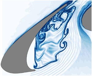
Figure 2. Mean vorticity contours with the superimposition of streamlines: (a) Re_c = 9.3 × 10³; (b) Re_c = 1.27 × 10⁴; (c) Re_c = 1.38 × 10⁴; (d) Re_c = 1.83 × 10⁴; (e) Re_c = 2.41 × 10⁴; (f) Re_c = 3.05 × 10⁴; (g) Re_c = 4.61 × 10⁴; (h) Re_c = 5.2 × 10⁴. The red dots mark the impingement locations of the slat cusp shear layer on the underside of the tailing edge. Although the mean vorticity contours in (b) and (d) have been reported by Wang et al. (Reference Wang, Feng, Wang and Li2018), it is still relevant to show them here for an integrated illustration of the effects of Re_c on the mean flow statistics.

Figure 3. Two-dimensional turbulent kinetic energy contours $(k/U_\infty ^2)$: (a) Re_c = 9.3 × 10³; (b) Re_c = 1.27 × 10⁴; (c) Re_c = 1.38 × 10⁴; (d) Re_c = 1.83 × 10⁴; (e) Re_c = 2.41 × 10⁴; (f) Re_c = 3.05 × 10⁴; (g) Re_c = 4.61 × 10⁴; (h) Re_c = 5.2 × 10⁴. The magenta crosses are located at the local peaks of $k/U_\infty ^2$. The fluctuations vertical to the main flow directions (v^tran) are extracted from these crosses to calculate the spectra in the current work.

4. Vortex dynamics

In this section, the effects of Re_c on the vortex dynamics around the slat are presented. It is found that three types of vortex dynamics occur to the slat cusp shear layer: (i) absence of vortex shedding (9.3 × 10³ ≤ Re_c ≤ 1.27 × 10⁴); (ii) impingement of shed vortices on the underside of the slat trailing edge at a steady location (1.38 × 10⁴ ≤ Re_c ≤ 1.83 × 10⁴); (iii) impingement of shed vortices on the underside of slat trailing edge at unsteady locations (2.41 × 10⁴ ≤ Re_c ≤ 5.2 × 10⁴). The typical LCSs and their links to the spectral properties in each type of vortex dynamics will be discussed in detail.

4.1. Absence of vortex shedding

The LCSs of the typical case of Re_c = 1.27 × 10⁴ are shown in figure 4(a–d). Consistent with Wang et al. (Reference Wang, Wang and Kim2019), no vortex shedding occurs to the slat cusp shear layer when Re_c ≤ 1.27 × 10⁴. The absence of vortex shedding leads to no obvious fluctuation around the reattachment location of the slat cusp shear layer. As a result, there is no obvious correlation between the reattachment location and the initial free shear layer around the slat cusp. In contrast, at Re_c = 1.38 × 10⁴, the spanwise shed vortex of the slat cusp shear layer (V_S in figure 4(e–h)) will impinge on the underside of the slat trailing edge and subsequently be cut into two parts by the trailing edge: one part passes through the gap region and is convected downstream; the other part is entrained into the recirculation as a vortex fluctuation (V_D in figure 4(e–h)). V_D will be convected by the recirculation to the slat cusp and further disturb the free shear layer. Consequently, a hydrodynamic feedback links the slat cusp and trailing edge. The vortex dynamics at Re_c = 1.38 × 10⁴ will be further discussed in the next subsection.

Figure 4. The LCSs revealed by the FTLEs method: (a–d) Re_c = 1.27 × 10⁴; (e–h) Re_c = 1.38 × 10⁴. Here, V_S denotes the shed vortex of the slat cusp shear layer; V_D denotes the vortex fluctuation produced by the impingement of V_S on the underside of the trailing edge; and Δt is chosen as the shedding period of V_S.

4.2. Impingement of shed vortices on the underside of the trailing edge at a steady location

Vortex shedding occurs to the slat cusp shear layer when Re_c ≥ 1.38 × 10⁴ (Wang et al. Reference Wang, Wang and Kim2019). Welch's method (Welch Reference Welch1967) is applied to the v^tran signals at the probes 1–5 of figure 3(c,d) to estimate the spectral properties of the slat cusp shear layer, which effectively reduces the effects of noise. The v^tran signal is first divided into 10 blocks with a 75 % overlapping Hanning window, which leads to 3595 data points in each block. The v^tran signal in each block is then transferred into a power spectral density by a fast Fourier transform. The power spectral densities of these 10 blocks are finally averaged to provide the power spectral densities in figure 5, which leads to a frequency resolution of 1/3595f_s (f_s is the sampling frequency of the CMOS camera). Figure 5 demonstrates the dominance of the fundamental frequency (St₁) and second harmonic (St₂) for 1.38 × 10⁴ ≤ Re_c ≤ 1.83 × 10⁴. The similar power spectral densities in figure 5(a,b) indicate the similar vortex dynamics of 1.38 × 10⁴ ≤ Re_c ≤ 1.83 × 10⁴. As mentioned by Wang et al. (Reference Wang, Wang and Kim2019), the formations and deformations of the shed vortices could be related to St₁ and St₂, respectively. At the early stage of the slat cusp shear layer (probe 1 in figure 5), only St₁ is remarkable. As the vortex shedding occurs, St₂ appears in the slat cusp shear layer (at probe 4 in figure 5(a) and probe 2 in figure 5(b)). Because the probes marked by the same number in figure 3 are located at similar vertical positions, figure 5 reveals the upstream move (to the slat cusp) of St₂ with increasing Re_c, coupled with the upstream move of vortex shedding (Wang et al. Reference Wang, Wang and Kim2019). In addition, the stronger shed vortices at Re_c = 1.83 × 10⁴ (owing to higher Re_c) lead to the stronger fundamental frequency and harmonics in figure 5(b) than those in figure 5(a). Notably, the PIV measurements at each Reynolds number are repeated three times to ensure the repeatability and reliability of the frequency peaks in figure 5.

Figure 5. Power spectral densities in the slat cusp shear layer: (a) Re_c = 1.38 × 10⁴; (b) Re_c = 1.83 × 10⁴. The local power spectral densities of 1–5 are calculated from the v^tran signals at the probes 1–5 of figure 3, respectively. St₁ and St₂ denote the fundamental frequency and second harmonic, respectively. The power spectral densities of each subfigure are amplified step by step by 10⁴ along the probe positions for clarity.

Figure 6 shows the wavelet spectra of the v^tran signals around the impingement location (1.38 × 10⁴ ≤ Re_c ≤ 1.83 × 10⁴). The dominant St₁ persists over the time interval, which indicates a good periodicity for the impingement of shed vortices on the underside of the trailing edge. The LCSs at Re_c = 1.38 × 10⁴ (figure 4e–h) and Re_c = 1.83 × 10⁴ (figure 7) further verify the good periodicity of the impingement. Similar to the case of Re_c = 1.38 × 10⁴, the vortex fluctuation (V_D in figure 7) links the slat cusp and trailing edge by a hydrodynamic feedback.

Figure 6. Wavelet spectra of the v^tran signals at probe 5 of figure 3: (a) Re_c = 1.38 × 10⁴; (b) Re_c = 1.83 × 10⁴. Here, St₁ and St₂ denote the fundamental frequency and second harmonic, respectively.

Figure 7. The LCSs revealed by the FTLEs method at Re_c = 1.83 × 10⁴. Here, V_S denotes the shed vortex of the slat cusp shear layer; V_D denotes the vortex fluctuation produced by the impingement of V_S on the underside of the trailing edge; and Δt is chosen as the shedding period of V_S.

4.3. Impingement of shed vortices on the underside of the trailing edge at unsteady locations

When 2.41 × 10⁴ ≤ Re_c ≤ 5.2 × 10⁴, the shed vortices of the slat cusp shear layer impinge on the underside of the trailing edge with unsteady impingement locations. Similar to the strategy of figure 5, Welch's method (Welch Reference Welch1967) is applied to the v^tran signals at the probes 1–5 of figure 3(e–h) to estimate the spectral properties of the slat cusp shear layer (figure 8), which effectively reduces the effects of noise. In addition to the fundamental frequency (St₁) and its harmonics (only the second one, St₂, is marked), subharmonics (St_0.*) and fractional harmonics (St_1.*) occur to the slat cusp shear layer (figure 8). Notably, the PIV measurements at each Reynolds number are repeated three times to ensure the repeatability and reliability of the frequency peaks in figure 8, although the subharmonics in figure 8(d) are indeed not prominent. The ‘imperfect’ peaks of subharmonics could be attributed to the insufficient sampling time of the v^tran signals, which is limited by the camera onboard memory during the PIV measurements. However, the ‘imperfect’ peaks do not affect the flow physics discussed in the current work, because the vortex shedding patterns related to these ‘imperfect’ peaks will be captured during the sampling time (§ 4.3.4). The Strouhal numbers (St = fc_s/U_∞) of St_0.* and St_1.* are found to be located around 1–5, similar to the narrowband peaks of the slat noise at Re_c ~ 10⁶ (Murayama et al. Reference Murayama, Nakakita, Yamamoto, Ura, Ito and Choudhari2014; Li et al. Reference Li, Liu, Guo, Hou, Geng and Wang2017; Pascioni & Cattafesta Reference Pascioni and Cattafesta2018a). It should be emphasized that the ratios of St_0.* to St₁ are located around 1/3St₁, 1/2St₁ and 2/3St₁, while the ratios of St_1.* to St₁ are located around 4/3St₁, 3/2St₁ and 5/3St₁. In addition to the universal law mentioned above, these subharmonics and fractional harmonics also show a Re_c-dependence to a certain extent. Therefore, the flow physics of these subharmonics and fractional harmonics will be discussed in this section for all the four typical Re_c. Accordingly, specific frequency bands are defined in figure 8 (marked by red dashed lines) to contain the fluctuations pertaining to these frequency peaks, further promoting the physical analyses of subharmonics and fractional harmonics. The quantitative intervals of these frequency bands are provided in table 1.

Figure 8. Power spectral densities in the slat cusp shear layer: (a) Re_c = 2.41 × 10⁴; (b) Re_c = 3.05 × 10⁴; (c) Re_c = 4.61 × 10⁴; (d) Re_c = 5.2 × 10⁴. The local power spectral densities of 1–5 are calculated from the v^tran signals at the probes 1–5 in figure 3, respectively. St₁ and St₂ denote the fundamental frequency and second harmonic, respectively. St_0.* and St_1.* denote the subharmonics and fractional harmonics, respectively. The red dashed lines define the frequency bands related to specific typical frequencies. The power spectral densities of each subfigure are amplified step by step by 10⁴ along the probe positions for clarity.

Table 1. The quantitative intervals of the frequency bands defined in figure 8.

4.3.1. The Re_c = 2.41 × 10⁴ case

The wavelet spectrum of the v^tran signal around the impingement locations is presented in figure 9. Similar to the cases of 1.38 × 10⁴ ≤ Re_c ≤ 1.83 × 10⁴, St₁ persists and dominates the spectrum over the time interval. In contrast, the subharmonic St_0.5 appears intermittently over the time interval. When St_0.5 is absent in the spectrum (t ₁ in figure 9), the impingement locations of two consecutive shed vortices are steady on the underside of the trailing edge (figure 10a,b), similar to the vortex dynamics of 1.38 × 10⁴ ≤ Re_c ≤ 1.83 × 10⁴. When St_0.5 is prominent in the spectrum (t ₂ in figure 9), most parts of the shed vortices in the former and latter cycles are respectively entrained into the recirculation of the slat cove and pushed through the gap (figure 10c,d), which lead to unsteady impingement locations on the underside of the trailing edge. Therefore, the subharmonic St_0.5 is related to the impingement of shed vortices with unsteady locations on the underside of the trailing edge.

Figure 9. Wavelet spectrum of the v^tran signal at probe 5 (figure 3) of Re_c = 2.41 × 10⁴. Here, St_0.5, St₁ and St₂ denote the subharmonic, fundamental frequency and second harmonic, respectively; and t ₁ and t ₂ mark the absent and prominent instances of St_0.5, respectively.

Figure 10. The LCSs revealed by the FTLEs method at Re_c = 2.41 × 10⁴. Here, V_S denotes the shed vortex of the free shear layer; t ₁ and t ₂ denote the absent and prominent instances of St_0.5, respectively; and Δt is chosen as the shedding period of V_S.

To gain additional insight into the flow physics of St_0.5, the reconstructed instantaneous fluctuations (v^tran) related to St_0.5 and St₁ are shown in figures 11 and 12, respectively. When St_0.5 is absent (t ₁ in figure 9), the fluctuations related to St_0.5 are weak in the slat cusp shear layer and the slat cove (figure 11a–d). When St_0.5 is prominent (t ₂ in figure 9), strong fluctuations related to St_0.5 appear in the slat cusp shear layer (figure 11e–h). As indicated by the pattern in figure 11(f) (marked by a magenta ellipse), the impingement with unsteady locations can generate fluctuations of St_0.5 and further disturb the slat cusp shear layer by the hydrodynamic feedback in the slat cove. Strong fluctuations of St₁ exist in the slat cusp shear layer regardless of whether St_0.5 is prominent or not (figure 12), which is consistent with the vortex shedding patterns in figure 10. As unveiled by the pattern in figure 12(b) (marked by a magenta ellipse), the fluctuations originating from the impingement with the fundamental frequency can also disturb the slat cusp shear layer by the hydrodynamic feedback in the slat cove. In summary, the amplification of the subharmonic (St_0.5) in the slat cusp shear layer leads to the shed vortices impinging on the underside of the trailing edge with unsteady impingement locations. The hydrodynamic feedback links the slat cusp and trailing edge.

Figure 11. The reconstructed instantaneous velocity fields (normalized by U_∞) related to St_0.5 at Re_c = 2.41 × 10⁴. Here, t ₁ and t ₂ denote the absent and prominent instances of St_0.5, respectively; and Δt is chosen as the shedding period of V_S. Only the fluctuation components vertical to the main flow directions (v^tran) are contained in the fluctuation reconstruction.

Figure 12. The reconstructed instantaneous velocity fields (normalized by U_∞) related to St₁ at Re_c = 2.41 × 10⁴. Here, t ₁ and t ₂ denote the absent and prominent instances of St_0.5, respectively; and Δt is chosen as the shedding period of V_S. Only the fluctuation components vertical to the main flow directions (v^tran) are contained in the fluctuation reconstruction.

4.3.2. The Re_c = 3.05 × 10⁴ case

As Re_c increases, more wavelet spectra at different probes are required to characterize the frequency properties of the slat cusp shear layer. Figure 13 shows the wavelet spectra extracted from the probes 5 and 3 in figure 3. The wavelet spectrum of probe 5 (figure 13a) is still employed to characterize the vortex dynamics around the impingement locations. According to the spectra in figure 8(b), the wavelet spectrum of probe 3 (figure 13b) is more suitable for characterizing the vortex dynamics at the early stage of the slat cusp shear layer. In figure 13(b), St₁ persists and dominates the spectrum over the time interval. The subharmonics (St_0.36 and St_0.67) and fractional harmonics (St_1.29 and St_1.67) have already appeared in the slat cusp shear layer intermittently. Around the impingement locations, St_0.36 and St_0.67 are intensified markedly and couple with each other (figure 13a). The vortex shedding pattern of St₁ is illustrated in figure 14(a) by the LCSs at t ₁ of figure 13(a), when St₁ is the only prominent frequency. It is found that two consecutive shed vortices of the slat cusp shear layer ($V_S^1$ and $V_S^2$ in figure 14(a)) exist in the gap flow. When St_0.36 and St_0.67 are prominent (t ₂ of figure 13(a)), there are still two consecutive shed vortices existing in the gap flow ($V_S^1$ and $V_S^2$ in figure 14(b–d)). The impingement locations of three consecutive shed vortices become unsteady: more of the first shed vortex is entrained into the recirculation of the slat cove ($V_S^1$ in figure 14(b)); more of the latter two shed vortices are pushed through the gap ($V_S^1$ in figure 14(c,d)). The instances of prominent St_1.29 (t ₃ of figure 13(b)) and St_1.67 (t ₄ of figure 13(b)) are found to contain three ($V_S^1$, $V_S^2$ and $V_S^3$ in figure 14(e)) and four ($V_S^1$, $V_S^2$, $V_S^3$ and $V_S^4$ in figure 14(f)) consecutive shed vortices in the gap flow, respectively. Therefore, the subharmonics are related to the impingement of shed vortices with unsteady locations on the underside of the trailing edge. The vortex shedding patterns related to the fractional harmonics contain more shed vortices in the gap flow than that of the fundamental frequency.

Figure 13. Wavelet spectra of the v^tran signals at different probes of Re_c = 3.05 × 10⁴: (a) probe 5 of figure 3; (b) probe 3 of figure 3. Here, St₁ and St₂ denote the fundamental frequency and second harmonic, respectively. Here, St_0.36 and St_0.67 denote the subharmonics; St_1.29 and St_1.67 denote the fractional harmonics; t ₁, t ₃ and t ₄ mark the typical instances of St₁, St_1.29 and St_1.67, respectively; and t ₂ marks the typical instant of St_0.36 and St_0.67.

Figure 14. The LCSs revealed by the FTLEs method at Re_c = 3.05 × 10⁴: (a) at instant t ₁ of figure 13; (b–d) at instant t ₂ of figure 13; (e) at instant t ₃ of figure 13; (f) at instant t ₄ of figure 13. Here, $V_S^1$, $V_S^2$, $V_S^3$ and $V_S^4$ denote the shed vortices of the free shear layer; and Δt is chosen as the period of shed vortex with fundamental frequency.

The reconstructed instantaneous fluctuations (v^tran) related to different specific frequencies (St₁, St_0.36, St_0.67, St_1.29 and St_1.67) are provided in figures 15–19. Figure 15 demonstrates that strong fluctuations pertaining to St₁ exist in the slat cusp shear layer regardless of whether the subharmonics and fractional harmonics are prominent or not. If the fully developed patterns with negative fluctuating velocities in figure 15 (marked by black ellipses) could be related to the discrete vortices identified in figure 14, two and only two vortices should exist in the gap flow of figure 14. However, this is not the case. Three and four discrete vortices exist in the gap flow of figures 14(e) and 14(f), respectively. Notably, the patterns of $V_S^1$ and $V_S^2$ in figure 14(e) and of $V_S^1$ and $V_S^3$ in figure 14(f) are comparable with those of $V_S^1$ and $V_S^2$ in figure 14(a). Therefore, the strong fluctuations in the slat cusp shear layer of figure 15(e) are attributed to the $V_S^1$ and $V_S^2$ in figure 14(e), while the strong fluctuations in the slat cusp shear layer of figure 15(f) are ascribed to the $V_S^1$ and $V_S^3$ in figure 14(f). Therefore, $V_S^3$ in figure 14(e) and $V_S^2$ and $V_S^4$ in figure 14(f) could be treated as the productions of the secondary instability in the braid region between two consecutive vortices (Smyth Reference Smyth2003). Additionally, the pattern in figure 15(a) (marked by a magenta ellipse) reveals the hydrodynamic feedback in the slat cove. The reconstructed instantaneous fluctuations pertaining to St_0.36 and St_0.67 are shown in figures 16 and 17, respectively. The unsteady impingement locations on the underside of the trailing edge (figure 14b–d) are found to correlate with the strong fluctuations related to St_0.36 (figure 16b–d) and St_0.67 (figure 17b–d) in the slat cusp shear layer. As shown in figure 13, the typical instance of St_1.67 (t ₄) also contains strong St_0.36 and St_0.67. Consequently, strong fluctuations related to St_0.36 and St_0.67 also appear in the slat cusp shear layer at t ₄ (figures 16f and 17f). These strong fluctuations could make the shed vortices in figure 14(f) have unsteady impingement locations on the underside of the trailing edge. Again, the patterns in figures 16(b–d) and 17(b–d) (marked by magenta ellipses) demonstrate that the impingement with unsteady locations can generate fluctuations of subharmonics and further disturb the slat cusp shear layer by the hydrodynamic feedback in the slat cove. The vortex shedding patterns in figures 14(e) and 14(f) are respectively attributed to the strong fluctuations pertaining to St_1.29 (figure 18) and St_1.67 (figure 19) in the slat cusp shear layer. Because the pattern of $V_S^1$, $V_S^3$ and $V_S^4$ in figure 14(f) is comparable to that of $V_S^1$, $V_S^2$ and $V_S^3$ in figure 14(e), strong fluctuations related to St_1.29 also appear in the slat cusp shear layer of figure 18(f). In summary, the amplification of the subharmonics (St_0.36 and St_0.67) in the slat cusp shear layer leads to the unsteady impingement locations when the shed vortices impinge on the underside of the trailing edge. The fractional harmonics (St_1.29 and St_1.67) could trigger the secondary instability of the braid region between two consecutive vortices, which generates more shed vortices in the gap flow. The hydrodynamic feedback still links the slat cusp and trailing edge.

Figure 15. The reconstructed instantaneous velocity fields (normalized by U_∞) related to St₁ at Re_c = 3.05 × 10⁴: (a) at instant t ₁ of figure 13; (b–d) at instant t ₂ of figure 13; (e) at instant t ₃ of figure 13; (f) at instant t ₄ of figure 13. Here, Δt is chosen as the period of shed vortex with fundamental frequency. Only the fluctuation components vertical to the main flow directions (v^tran) are contained in the fluctuation reconstruction.

Figure 16. The reconstructed instantaneous velocity fields (normalized by U_∞) related to St_0.36 at Re_c = 3.05 × 10⁴: (a) at instant t ₁ of figure 13; (b–d) at instant t ₂ of figure 13; (e) at instant t ₃ of figure 13; (f) at instant t ₄ of figure 13. Here, Δt is chosen as the period of shed vortex with fundamental frequency. Only the fluctuation components vertical to the main flow directions (v^tran) are contained in the fluctuation reconstruction.

Figure 17. The reconstructed instantaneous velocity fields (normalized by U_∞) related to St_0.67 at Re_c = 3.05 × 10⁴: (a) at instant t ₁ of figure 13; (b–d) at instant t ₂ of figure 13; (e) at instant t ₃ of figure 13; (f) at instant t ₄ of figure 13. Here, Δt is chosen as the period of shed vortex with fundamental frequency. Only the fluctuation components vertical to the main flow directions (v^tran) are contained in the fluctuation reconstruction.

Figure 18. The reconstructed instantaneous velocity fields (normalized by U_∞) related to St_1.29 at Re_c = 3.05 × 10⁴: (a) at instant t ₁ of figure 13; (b–d) at instant t ₂ of figure 13; (e) at instant t ₃ of figure 13; (f) at instant t ₄ of figure 13. Here, Δt is chosen as the period of shed vortex with fundamental frequency. Only the fluctuation components vertical to the main flow directions (v^tran) are contained in the fluctuation reconstruction.

Figure 19. The reconstructed instantaneous velocity fields (normalized by U_∞) related to St_1.67 at Re_c = 3.05 × 10⁴: (a) at instant t ₁ of figure 13; (b–d) at instant t ₂ of figure 13; (e) at instant t ₃ of figure 13; (f) at instant t ₄ of figure 13. Here, Δt is chosen as the period of shed vortex with fundamental frequency. Only the fluctuation components vertical to the main flow directions (v^tran) are contained in the fluctuation reconstruction.

4.3.3. The Re_c = 4.61 × 10⁴ case

Following the methodology of figure 13, the wavelet spectra extracted from the probes 5 and 2 in figure 3 are provided in figure 20. St₁ still persists and dominates the spectrum over the time interval in figure 20(b). Additionally, the subharmonics (St_0.29, St_0.51 and St_0.78) and fractional harmonics (St_1.29, St_1.53 and St_1.82) intermittently appear in figure 20(b). Similar to the case of Re_c = 3.05 × 10⁴, the subharmonics are markedly intensified around the impingement locations (figure 20a). The LCSs in figure 21(a) demonstrate the vortex shedding pattern of St₁ (t ₁ of figure 20(a)). It is found that three shed vortices coexist in the gap flow ($V_S^1$, $V_S^2$ and $V_S^3$ in figure 21(a)). Similar to the case of Re_c = 3.05 × 10⁴, St_0.29 and St_0.78 correlate with the impingement of shed vortices with unsteady impingement locations: more of the first shed vortex is entrained into the recirculation of slat cove ($V_S^1$ in figure 21(b)); more of the latter two shed vortices are pushed through the gap ($V_S^1$ in figure 21(c,d)). For the typical instance of St_0.51 (t ₃ of figure 20(a)), the shed vortices of the slat cusp shear layer still impinge on the underside of the trailing edge with unsteady impingement locations (figure 21e–h). The unsteady behaviour of the impingement locations in figure 21(e–h) is comparable to that pertaining to St_0.5 at Re_c = 2.41 × 10⁴ (figure 10c,d). When St_1.29 is prominent (t ₄ of figure 20(b)), four shed vortices coexist in the gap flow ($V_S^1$, $V_S^2$, $V_S^3$ and $V_S^4$ in figure 21(i)). As expected, the gap flow contains five shed vortices ($V_S^1$, $V_S^2$, $V_S^3$, $V_S^4$ and $V_S^5$ in figure 21(j)) when St_1.82 is prominent (t ₅ of figure 20(b)). Compared with those at Re_c = 2.41 × 10⁴ and Re_c = 3.05 × 10⁴, the instantaneous fluctuation reconstructions at Re_c = 4.61 × 10⁴ reveal similar flow physics and will not be shown for conciseness.

Figure 20. Wavelet spectra of the v^tran signals at different probes of Re_c = 4.61 × 10⁴: (a) probe 5 of figure 3; (b) probe 2 of figure 3. Here, St₁ and St₂ denote the fundamental frequency and second harmonic, respectively; St_0.29, St_0.51 and St_0.78 denote the subharmonics; St_1.29, St_1.53 and St_1.82 denote the fractional harmonics; t ₁, t ₄ and t ₅ mark the typical instances of St₁, St_1.29 and St_1.82, respectively; t ₂ marks the typical instant of St_0.29 and St_0.78; and t ₃ marks the typical instant of St_0.51.

Figure 21. The LCSs revealed by the FTLEs method at Re_c = 4.61 × 10⁴: (a) at instant t ₁ of figure 20; (b–d) at instant t ₂ of figure 20; (e–h) at instant t ₃ of figure 20; (e) at instant t ₄ of figure 20; (f) at instant t ₅ of figure 20. Here, $V_S^1$, $V_S^2$, $V_S^3$, $V_S^4$ and $V_S^5$ denote the shed vortices of the free shear layer; and Δt is chosen as the period of shed vortex with fundamental frequency.

In summary, the amplification of subharmonics (St_0.29, St_0.51 and St_0.78) in the slat cusp shear layer leads to the unsteady impingement locations when the shed vortices impinge on the underside of the trailing edge. By triggering the secondary instability of the braid region, the fractional harmonics (St_1.29 and St_1.82) in the slat cusp shear layer could generate more shed vortices in the gap flow. The hydrodynamic feedback still links the slat cusp and trailing edge. It should be mentioned that the fractional harmonic of St_1.53 is too weak to trigger the secondary instability of the braid region. Therefore, no specific vortex shedding pattern related to St_1.53 is captured in the current work.

4.3.4. The Re_c = 5.2 × 10⁴ case

The wavelet spectra at probes 5 and 2 are presented in figure 22. At the early stage of the slat cusp shear layer, the dominant frequency switches between the fundamental frequency St₁ and the fractional harmonic St_1.31 (figure 22b), similar to the mode switching of the narrowband peaks at Re_c ~ 10⁶ (Li et al. Reference Li, Liu, Xing and Guo2018a). Except for the time interval of 0.5–1.5 s, the left time interval in figure 22(b) is still dominated by St₁. In addition, the subharmonics (St_0.36 and St_0.63) and another fractional harmonic (St_1.69) intermittently appear in the slat cusp shear layer at the early stage (figure 22b). Similar to the cases of Re_c = 3.05 × 10⁴ and Re_c = 4.61 × 10⁴, the subharmonics are markedly intensified around the impingement locations (figure 22a). The LCSs in figure 23(a) show that three shed vortices ($V_S^1$, $V_S^2$ and $V_S^3$) coexist in the gap flow at the typical instance of St₁ (t ₁ in figure 22(a)). The subharmonics are found to correlate with the impingement of shed vortices with unsteady impingement locations (figure 23b–d), similar to the scenarios of Re_c = 2.41 × 10⁴, Re_c = 3.05 × 10⁴ and Re_c = 4.61 × 10⁴. For the typical instance of St_1.31 (t ₃ in figure 22(b)), the gap flow simultaneously contains four shed vortices ($V_S^1$, $V_S^2$, $V_S^3$ and $V_S^4$ in figure 23(e)). While for the typical instance of St_1.69 (t ₄ in figure 22(b)), there are five shed vortices ($V_S^1$, $V_S^2$, $V_S^3$, $V_S^4$ and $V_S^5$ in figure 23(f)) in the gap flow. The instantaneous fluctuation reconstructions are still employed to add more insights into the specific frequencies mentioned above. The resulted conclusions at Re_c = 5.2 × 10⁴ are strongly similar to those at Re_c = 2.41 × 10⁴, Re_c = 3.05 × 10⁴ and Re_c = 4.61 × 10⁴. As a result, the reconstructed instantaneous fluctuations are not provided here for conciseness.

Figure 22. Wavelet spectra of the v^tran signals at different probes of Re_c = 5.2 × 10⁴: (a) probe 5 of figure 3; (b) probe 2 of figure 3. Here, St₁ and St₂ denote the fundamental frequency and second harmonic, respectively; St_0.36 and St_0.63 denote the subharmonics; St_1.31 and St_1.69 denote the fractional harmonics; t ₁, t ₃ and t ₄ mark the typical instances of St₁, St_1.31 and St_1.69, respectively; and t ₂ marks the typical instant of St_0.36 and St_0.63.

Figure 23. The LCSs revealed by the FTLEs method at Re_c = 5.2 × 10⁴: (a) at instant t ₁ of figure 22; (b–d) at instant t ₂ of figure 22; (e) at instant t ₃ of figure 22; (f) at instant t ₄ of figure 22. Here, $V_S^1$, $V_S^2$, $V_S^3$, $V_S^4$ and $V_S^5$ denote the shed vortices of the free shear layer; and Δt is chosen as the period of shed vortex with fundamental frequency.

In summary, the strong fluctuations of St_0.36 and St_0.63 in the slat cusp shear layer make the shed vortices have unsteady impingement locations on the underside of the trailing edge. St_1.31 and St_1.69 in the slat cusp shear layer contribute to more shed vortices in the gap flow by triggering the secondary instability of the braid region. The mode switching in the spectra of the slat flow is attributed to the switching between different vortex shedding patterns of the slat cusp shear layer. The hydrodynamic feedback links the slat cusp and trailing edge.

5. Extending the vortex dynamics to high Reynolds numbers

The links of slat flows between low and high Reynolds numbers will be discussed in this section. As reported by Murayama et al. (Reference Murayama, Nakakita, Yamamoto, Ura, Ito and Choudhari2014), Pascioni & Cattafesta (Reference Pascioni and Cattafesta2016) and Li et al. (Reference Li, Liu, Xing and Guo2018b), the dimensional frequencies of the narrowband peaks at Re_c ~ 10⁶ are approximately 10³ Hz, which are higher than those in the current work (~10¹ Hz). However, the non-dimensional Strouhal numbers of these narrowband peaks in the current work (approximately 1–5 in figure 8) are comparable to those at Re_c ~ 10⁶, which strongly indicates the potential relations between the slat flows at Re_c ~ 10⁴ and Re_c ~ 10⁶. The discussions in this section indicate that the vortex dynamics in the range of 2.41 × 10⁴ ≤ Re_c ≤ 5.2 × 10⁴ could persist to the range of Re_c ~ 10⁶.

The ratios of other typical frequencies to the fundamental frequency are presented in figure 24. All benchmark databases at Re_c ~ 10⁶ of figure 24 show the investigations at the geometric angles of attack comparable to the current work. Notably, the slight deviations of geometric angle of attack between the benchmark databases and the current work do not affect the flow physics revealed by figure 24, because narrowband peaks robustly exist in the spectra with different angles of attack to a certain extent (Kolb et al. Reference Kolb, Faulhaber, Drobietz and Grünewald2007; Imamura et al. Reference Imamura, Ura, Yokokawa and Yamamoto2009; Murayama et al. Reference Murayama, Nakakita, Yamamoto, Ura, Ito and Choudhari2014; Herr et al. Reference Herr, Pott-Pollenske, Ewert, Boenke, Siebert, Delfs, Rudenko, Büscher, Friedel and Mariotti2015; Pagani, Souza & Medeiros Reference Pagani, Souza and Medeiros2016, Reference Pagani, Souza and Medeiros2017). Surprisingly, the subharmonics and fractional harmonics observed in the range of 2.41 × 10⁴ ≤ Re_c ≤ 5.2 × 10⁴ still exist in the slat flow at Re_c ~ 10⁶. Moreover, the ratios of subharmonics to the fundamental frequency are located around 1/3St₁, 1/2St₁ and 2/3St₁, while the ratios of fractional harmonics to the fundamental frequency are located around 4/3St₁, 3/2St₁ and 5/3St₁. This universal law indicates that the vortex dynamics in the current low-Reynolds-number range (2.41 × 10⁴ ≤ Re_c ≤ 5.2 × 10⁴) could persist to the high-Reynolds-number range (Re_c ~ 10⁶). This conjecture can be further verified by the massive similarities of the vortex dynamics between low and high Reynolds numbers:

1. (i) In the range of 2.41 × 10⁴ ≤ Re_c ≤ 5.2 × 10⁴, the shed vortices of the slat cusp shear layer can impinge on the underside of the trailing edge with unsteady impingement locations, similar to the scenario where the shed vortices could be either entrained into the recirculation of slat cove or pushed through the gap at Re_c ~ 10⁶ (Jenkins et al. Reference Jenkins, Khorrami and Choudhari2004; Deck & Laraufie Reference Deck and Laraufie2013).

2. (ii) When Re_c ≥ 4.61 × 10⁴, the single-recirculation pattern in the slat cove is comparable with the topology of the slat cove at Re_c ~ 10⁶ (Jenkins et al. Reference Jenkins, Khorrami and Choudhari2004; Pascioni et al. Reference Pascioni, Cattafesta and Choudhari2014). As mentioned in § 3, the slat cusp shear layer reattaches on the underside of the trailing edge. The distance between the trailing edge and the reattachment location is estimated to be 0.1c_s at Re_c = 5.2 × 10⁴, which is consistent with the estimation of Jenkins et al. (Reference Jenkins, Khorrami and Choudhari2004) at Re_c = 3.64 × 10⁶.

3. (iii) As visualized by the λ ₂ criterion, four large-scale shed vortices coexist in the gap flow of Souza et al. (Reference Souza, Rodríguez, Himeno and Medeiros2019) (Re_c = 1 × 10⁶). The gap flow at Re_c = 5.2 × 10⁴ can also contain four large-scale shed vortices according to the LCSs extracted by the FTLEs method.

4. (iv) Li et al. (Reference Li, Liu, Xing and Guo2018a) observed the mode switching of the narrowband peaks in the far-field noise spectrum at Re_c ~ 10⁶. It is found that mode switching also occurs to the vortex shedding patterns of the slat cusp shear layer at Re_c = 5.2 × 10⁴.

Figure 24. Ratios of other typical frequencies to the fundamental frequency.

Notably, Pascioni & Cattafesta (Reference Pascioni and Cattafesta2018a,Reference Pascioni and Cattafestab) reported that a low frequency peak existed in the surface pressure spectra near the reattachment point of the slat cusp shear layer at Re_c ~ 10⁶. The frequency of this special peak was one order of magnitude lower than the fundamental frequency (St₁), which led to the related Strouhal number of approximately 0.1St₁. The phase-averaged results of Pascioni & Cattafesta (Reference Pascioni and Cattafesta2018b) indicated that the fundamental frequency was related to the shed vortices of the slat cusp shear layer. The modal analyses by Pascioni & Cattafesta (Reference Pascioni and Cattafesta2018b) revealed that the low frequency peak (0.1St₁) was attributed to the flapping, rather than the shed vortices, of the slat cusp shear layer. In contrast, figures 11, 16 and 17 indicate that the subharmonics are related to the shed vortices of the slat cusp shear layer. Therefore, the flow physics of the low frequency peak (0.1St₁) reported by Pascioni & Cattafesta (Reference Pascioni and Cattafesta2018a,Reference Pascioni and Cattafestab) is different from that of the subharmonics in the current work, although these two kinds of frequency peaks can lead to similarly unsteady reattachment (or impingement) of the slat cusp shear layer on the underside of the slat trailing edge. Unfortunately, the low frequency peak (0.1St₁) reported by Pascioni & Cattafesta (Reference Pascioni and Cattafesta2018a,Reference Pascioni and Cattafestab) is too low to be captured in the current measurements, because the recording time of PIV is limited by the onboard memory of the camera. As a result, the effects of shear layer flapping on the vortex dynamics of slat flows cannot be discussed in the current work.

According to Terracol et al. (Reference Terracol, Manoha and Lemoine2015) and Souza et al. (Reference Souza, Rodríguez, Himeno and Medeiros2019), the narrowband peaks at Re_c ~ 10⁶ should be attributed to the aeroacoustic feedback in the slat cove. The shed vortices of the slat cusp shear layer impinge on the underside of the trailing edge and generate fluctuations around the impingement locations. These fluctuations are convected to the slat cusp with the speed of sound. Consequently, the aeroacoustic feedback links the slat cusp and trailing edge. While for the current low-Reynolds-number case, the fluctuations, which originate from the impingement of shed vortices on the underside of the trailing edge, are convected to the slat cusp with the speed of the recirculation in the slat cove. As a result, a hydrodynamic feedback links the slat cusp and trailing edge. It seems like different kinds of feedback lead to similar narrowband peaks. The relations between the aeroacoustic feedback and the hydrodynamic feedback are therefore discussed here to figure out this ‘contradiction’:

1. (i) The aeroacoustic feedback and the hydrodynamic feedback are intrinsically similar. The fluctuations for feedback in these two mechanisms both originate from the interactions between the shed vortices of the slat cusp shear layer and the underside surface of the slat trailing edge (Dobrzynski Reference Dobrzynski2010; Deck & Laraufie Reference Deck and Laraufie2013; Terracol et al. Reference Terracol, Manoha and Lemoine2015; Pascioni & Cattafesta Reference Pascioni and Cattafesta2018b; Souza et al. Reference Souza, Rodríguez, Himeno and Medeiros2019). The aeroacoustic feedback reported by Terracol et al. (Reference Terracol, Manoha and Lemoine2015) and Souza et al. (Reference Souza, Rodríguez, Himeno and Medeiros2019) could be generally treated as a kind of hydrodynamic feedback, if the traveling speed of fluctuations (sound speed) is replaced by the speed of the recirculation in the slat cove.

2. (ii) The different feedback speeds between the aeroacoustic feedback and the hydrodynamic feedback do not affect the non-dimensional Strouhal numbers of narrowband peaks. The selection of narrowband peaks in the current hydrodynamic feedback is similar to that in the aeroacoustic feedback at Re_c ~ 10⁶. The prediction equation for narrowband peaks $(\,{f_n})$ in the aeroacoustic feedback, improved by Terracol et al. (Reference Terracol, Manoha and Lemoine2015), is

   (5.1)\begin{equation}{f_n} = ({n_a} + {n_v})\frac{{{U_v}({c_0} - {U_a})}}{{{L_a}{U_v} + {L_v}({c_0} - {U_a})}},\end{equation}

   where ${U_v}$ is the convection velocity of the fluctuations in the slat cusp shear layer, ${c_0}$ is the speed of sound, ${U_a}$ is the mean velocity component inside the slat cove and is opposite to the convection direction of returning acoustic fluctuations, ${L_v}$ and ${L_a}$ are respectively the shear layer length and the acoustic feedback path, ${n_a}$ is the wavenumber of the returning acoustic fluctuations in the slat cove, ${n_v}$ is the wavenumber of the fluctuations in the slat cusp shear layer. Compared with ${c_0}$, ${U_a}$ has negligible effects on the acoustic feedback path and therefore can be neglected. The non-dimensional prediction equation (using the freestream velocity ${U_\infty }$ and the slat chord length ${c_s}$) is then written as

   (5.2)\begin{equation}\textrm{S}{\textrm{t}_n} = ({n_a} + {n_v}){\left( {\frac{{{L_a}}}{{{c_s}}}\frac{{{U_\infty }}}{{{c_0}}} + \frac{{{L_v}}}{{{c_s}}}\frac{{{U_\infty }}}{{{U_v}}}} \right)^{ - 1}}.\end{equation}

   The large feedback speed $({c_0})$ can immediately convect the fluctuations around the slat trailing edge to the slat cusp, which leads to the term of ${U_\infty }/{c_0}$ in (5.2) of around 0.1 (Terracol et al. Reference Terracol, Manoha and Lemoine2015; Souza et al. Reference Souza, Rodríguez, Himeno and Medeiros2019). As a result, the slat cusp shear layer can be disturbed by the fluctuations around the slat trailing edge in a rapid manner at Re_c ~ 10⁶. The ${n_a}$ in (5.2) therefore equals 1 for the aeroacoustic feedback, which is supported by figure 22 of Souza et al. (Reference Souza, Rodríguez, Himeno and Medeiros2019). Following the strategies of Terracol et al. (Reference Terracol, Manoha and Lemoine2015), the non-dimensional prediction equation for the current hydrodynamic feedback could be proposed as

   (5.3)\begin{equation}\textrm{S}{\textrm{t}_n} = ({n_h} + {n_v}){\left( {\frac{{{L_h}}}{{{c_s}}}\frac{{{U_\infty }}}{{{U_h}}} + \frac{{{L_v}}}{{{c_s}}}\frac{{{U_\infty }}}{{{U_v}}}} \right)^{ - 1}}.\end{equation}

   The feedback speed of ${c_0}$, the acoustic feedback path ${L_a}$ and the wavenumber of the returning acoustic fluctuations in the slat cove ${n_a}$ in (5.2) are replaced by the speed of recirculation ${U_h}$, the hydrodynamic feedback path ${L_h}$ and the wavenumber of the returning hydrodynamic fluctuations in the slat cove ${n_h}$ in (5.3), respectively. Because of the small value of ${U_h}$, the term of ${U_\infty }/{U_h}$ in (5.3) is estimated to be approximately 5 for the current hydrodynamic feedback, which is larger than the term of ${U_\infty }/{c_0}$ in (5.2). As a result, the fluctuations around the slat trailing edge need a longer time to be convected to the slat cusp at Re_c ~ 10⁴. Therefore, there is a time delay for the fluctuations around the slat trailing edge to disturb the slat cusp shear layer at Re_c ~ 10⁴. Notably, the fluctuations for hydrodynamic feedback originate from the interactions between the shed vortices of the slat cusp shear layer and the underside surface of the slat trailing edge at Re_c ~ 10⁴. Although the slat cusp shear layer cannot be immediately disturbed by the fluctuations generated in the current vortex shedding cycle, it can immediately be disturbed by the fluctuations generated in some former vortex shedding cycle. Because the periodic vortex shedding related to a specific narrowband peak can robustly persist for a period, the fluctuations with similar frequency properties fill the feedback path in the slat cove (figures 11–12 and 15–17). As a result, the slat cusp shear layer can immediately be disturbed by the fluctuations comparable to those generated in the current vortex shedding cycle. Therefore, the term of ${n_h}$ in (5.3) is larger than 3 for the current hydrodynamic feedback (figures 11–12 and 15–17), which is larger than the ${n_a}$ in (5.2). Except for the two terms of ${n_a}$ and ${U_\infty }/{c_0}$ in (5.2) and of ${n_h}$ and ${U_\infty }/{U_h}$ in (5.3), the other terms in these two equations have comparable values (supported by the current results and the results reported by Terracol et al. (Reference Terracol, Manoha and Lemoine2015) and Souza et al. (Reference Souza, Rodríguez, Himeno and Medeiros2019)). As a result, the large ${n_h}$ and ${U_\infty }/{U_h}$ in (5.3) still lead to a $\textrm{S}{\textrm{t}_n}$ around 1–5, comparable to that of (5.2). Therefore, the different feedback speeds do not change the intrinsic similarity between the aeroacoustic feedback and the hydrodynamic feedback. The coupled variations of the feedback fluctuation wavenumber (${n_a}$ in (5.2) and ${n_h}$ in (5.3)) and the feedback speed (${U_\infty }/{c_0}$ in (5.2) and ${U_\infty }/{U_h}$ in (5.3)) result in similar non-dimensional Strouhal numbers between the aeroacoustic feedback and the current hydrodynamic feedback. Although the amplitudes of the returning hydrodynamic fluctuations in the slat cove could be sufficiently high to trigger the instability of the slat cusp shear layer, they are too low to accurately determine the ${n_h}$ in (5.3). Therefore, (5.3) fails to accurately predict the narrowband peaks in figure 8. Reliable time-resolved databases of the slat flows, with higher accuracy to determine the ${n_h}$ in (5.3), should be pursued in future work to improve (5.3).

3. (iii) The shed vortices of the slat cusp shear layer at Re_c ~ 10⁶ (aeroacoustic feedback) should contain more turbulence than those at Re_c ~ 10⁴ (hydrodynamic feedback). However, this difference does not affect the non-dimensional Strouhal numbers of the narrowband peaks. Souza et al. (Reference Souza, Rodríguez, Himeno and Medeiros2019) found that the large-scale shed vortices, rather than the small-scale turbulence, were relevant to the radiation of narrowband peaks. Because the vortex dynamics of Re_c ~ 10⁶ and Re_c ~ 10⁴ are found to be comparable with each other in large-scale flow structures, the narrowband peaks related to these two kinds of feedback should have similar non-dimensional Strouhal numbers.

4. (iv) The aeroacoustic feedback and the hydrodynamic feedback can coexist or couple with each other at Re_c ~ 10⁴ and Re_c ~ 10⁶. Although they cannot be captured in the current measurements, the pressure waves, generated by the impingement of shed vortices on the underside of trailing edge, are expected to be convected to the slat cusp with the speed of sound at Re_c ~ 10⁴. This kind of process can therefore be depicted by (5.2). Owing to the large value of ${c_0}$ (${c_0} \approx 1500\;\textrm{m}\;{\textrm{s}^{ - 1}} \gg {U_\infty }$), the term related to ${U_\infty }/{c_0}$ can be neglected and ${n_a}$ equals 0. As a result, (5.2) can be simplified and manipulated as

   (5.4)\begin{equation}\textrm{S}{\textrm{t}_n} = {n_v}{\left( {\frac{{{L_v}}}{{{c_s}}}\frac{{{U_\infty }}}{{{U_v}}}} \right)^{ - 1}} = {n_v}{\left( {\frac{{{L_v}}}{{{U_v}}}\frac{{{U_\infty }}}{{{c_s}}}} \right)^{ - 1}} = {n_v}{\left( {{t_v}\frac{{{U_\infty }}}{{{c_s}}}} \right)^{ - 1}},\end{equation}
   where ${t_v}$ is the convection time of disturbances inside the slat cusp shear layer from the slat cusp to the trailing edge and is directly calculated from the current time-resolved measurements. Similar to (5.3), (5.4) is also found to provide a predicted $\textrm{S}{\textrm{t}_n}$ around 1–5, which indicates the potential effects of aeroacoustic feedback at Re_c ~ 10⁴. However, many investigations have reported that the shed vortices of the slat cusp shear layer can be entrained into the recirculation in the slat cove and further convected to the slat cusp at Re_c ~ 10⁶ (Jenkins et al. Reference Jenkins, Khorrami and Choudhari2004; Choudhari & Khorrami Reference Choudhari and Khorrami2007; Deck & Laraufie Reference Deck and Laraufie2013), similar to the scenario of the current hydrodynamic feedback. It is therefore deduced that the hydrodynamic feedback discussed in the current work can persist to the range of Re_c ~ 10⁶ and coexist with the aeroacoustic feedback. However, how these two kinds of feedback couple with each other still needs to be further investigated with time-resolved databases at Re_c ~ 10⁶. Notably, Choudhari & Khorrami (Reference Choudhari and Khorrami2007) found that some recirculating structures can mainly trigger the three-dimensional instability of the shed vortices formed near the slat cusp, rather than trigger the vortex shedding of the slat cusp shear layer. However, this does not mean that all recirculating structures and acoustic waves inside the slat cove will destroy the shed vortices of the slat cusp shear layer and weaken/vanish the narrowband peaks. Some other recirculating structures and acoustic waves are conjectured to trigger the vortex shedding of the slat cusp shear layer and therefore contribute to the feedback in the slat cove. This conjecture is supported by Souza et al. (Reference Souza, Rodríguez, Himeno and Medeiros2019). Souza et al. (Reference Souza, Rodríguez, Himeno and Medeiros2019) found that two-dimensional large-scale shed vortices played an important role in the aeroacoustic feedback at Re_c ~ 10⁶, although the slat cove flow was strongly three-dimensional. The current work also supports this conjecture. Notably, the current recirculation inside the slat cove is strongly three-dimensional and contains complex recirculating structures, some of which may also be responsible for the three-dimensional instability of the shed vortices originating from the slat cusp shear layer. This kind of three-dimensional flow physics is beyond the scope of the current two-dimensional measurements. However, figures 11–12 and 15–17 present the reconstructed velocity fields within the frequency bands related to narrowband peaks and therefore show the recirculating structures with two-dimensionality. This kind of two-dimensional recirculating structures plays an important role in the current hydrodynamic feedback and is expected to persist to Re_c ~ 10⁶.

In summary, the strong evidence from the current work and in the literature have been discussed in this section to show that the vortex dynamics in the range of 2.41 × 10⁴ ≤ Re_c ≤ 5.2 × 10⁴ can persist to the range of Re_c ~ 10⁶. The feedback mechanisms at Re_c ~ 10⁴ and Re_c ~ 10⁶ are intrinsically similar and responsible for the narrowband peaks. However, these conclusions still need further verifications. Reliable time-resolved databases of the slat flows at Re_c = 10⁵–10⁶ should be pursued in future work to verify these conclusions.