


1. Introduction
Among different fluid–structure interaction problems, the problem of the unsteady hydrodynamics of an elastic plate oscillating under water has been under the scrutiny of numerous researchers due to its fundamental aspects and diverse practical applications (Sfakiotakis, Lane & Davies Reference Sfakiotakis, Lane and Davies1999; Dowell & Hall Reference Dowell and Hall2001; Amabili & Paidoussis Reference Amabili and Paidoussis2003; Chen et al. Reference Chen, Wu, Cui and Jensen2006; Shelley & Zhang Reference Shelley and Zhang2011; Hou, Wang & Layton Reference Hou, Wang and Layton2012). The challenging physics in this problem arises from the dynamic coupling between the elastic deformation of the plate and the unsteady fluid motion. As an elastic plate oscillates in a fluid, it bends due to its own inertia, elastic forces and hydrodynamic forces, yielding complex dynamic shape changes. The plate dynamics, in turn, imposes the motion on the viscous fluid surrounding the plate. Thus, the coupling between the plate dynamic deformation and the unsteady hydrodynamic loading needs to be resolved to understand the plate motion and to rationalize the resulting hydrodynamic forces associated with complex three-dimensional flow structures generated by the oscillating plate.
Most biological systems involved in flying or swimming consist of deformable surfaces actuated with muscle contractions and passive deformation due to the surrounding flow (Fish & Lauder Reference Fish and Lauder2006). In the case of swimming, fish are able to achieve swimming velocities, maximum burst speeds and efficiencies far exceeding the best man-made designs of comparable size (Scaradozzi et al. Reference Scaradozzi, Palmieri, Costa and Pinelli2017). Elasticity is often used by animals to generate complex deformation patterns using simple actuation (Jayne & Lauder Reference Jayne and Lauder1995; McHenry, Pell & Long Reference McHenry, Pell and Long1995; Lauder & Tytell Reference Lauder and Tytell2005). Multiple studies explored the movement of fish fins that undergo complex and inherently three-dimensional motion (Flammang & Lauder Reference Flammang and Lauder2009; Esposito et al. Reference Esposito, Tangorra, Flammang and Lauder2012; Lauder & Tangorra Reference Lauder and Tangorra2015). Through this complex motion and local change in elasticity, fish can achieve efficient swimming and manoeuvring.
Small and medium size fish measure up to 10–20 cm and reach swimming velocities up to several body lengths per second leading to Reynolds number  $Re \sim 10^{2} \text {--}10^{5}$. In this range of Reynolds number both inertial and viscous effects play a substantial role in the physics of the problem. Although the Reynolds number in this range is close to the critical value, Anderson, Mcgillis & Grosenbaugh (Reference Anderson, Mcgillis and Grosenbaugh2001) showed experimentally that the flow attached to the fish remains laminar.
An oscillating plate is an efficient simplified model representing the complex fluid mechanics of fish fins (Combes & Daniel Reference Combes and Daniel2001; Liu & Aono Reference Liu and Aono2009; Kolomenskiy et al. Reference Kolomenskiy, Moffatt, Farge and Schneider2011; Alben et al. Reference Alben, Witt, Baker, Anderson and Lauder2012). Exploring the hydrodynamics of oscillating plates enables researchers to better understand fish locomotion and to create efficient and manoeuvrable designs for biomimetic underwater swimmers. Early designs of fish-inspired robots include passive rigid or moderately elastic plates of various shapes actuated by servomotors (Triantafyllou & Triantafyllou Reference Triantafyllou and Triantafyllou1995; Anderson et al. Reference Anderson, Streitlien, Barrett and Triantafyllou1998). Some designs successfully mimicked the fish flexibility through a series of linked rigid sections coupled to actuators (Su et al. Reference Su, Yu, Tan and Zhang2014). Although such design proved to be successful in propelling robots, not only was the manoeuvring limited compared with what is seen in nature, but the efficiency was far from what fish achieve (Hu et al. Reference Hu, Liu, Dukes and Francis2006; Kopman et al. Reference Kopman, Laut, Acquaviva, Rizzo and Porfiri2015).
Recently, internally actuated smart materials have been developed and used to mimic complex fish-like motion showing a great potential for the development of efficient biomimetic swimming robots (Chen, Shatara & Tan Reference Chen, Shatara and Tan2009; Chen et al. Reference Chen, Um, Zhu and Bart-Smith2011; Philen & Neu Reference Philen and Neu2011). Among internally actuated smart materials, piezoelectric materials have gained significant interest. Particularly, macrofibre composite (MFC) piezoelectric actuators strike a balance between the actuation force and deformation levels, in addition to offering robust design and silent operation (Erturk & Delporte Reference Erturk and Delporte2011). The use of smart materials significantly simplifies the design of bioinspired robotic swimmers. Cen & Erturk (Reference Cen and Erturk2013) demonstrated a robotic fish propelled by MFC bimorphs, which consists of two MFC laminates bonded together by a layer of epoxy. While MFC bimorphs and other smart materials are highly promising solutions for driving bioinspired designs, they still yield somewhat limited deflection magnitude during underwater actuation due to hydrodynamic loads. Furthermore, it is unclear at what hydrodynamic regimes such materials need to be used to induce efficient locomotion and how their hydrodynamic performance compares with more traditional propulsors actuated by external driving mechanisms.
The problem of elastic plates oscillating in fluid is not limited to the biological and biomimetic locomotion. This fundamental problem has direct implications to a wide range of engineering applications including energy harvesting (Erturk & Inman Reference Erturk and Inman2011; Cha, Kim & Porfiri Reference Cha, Kim and Porfiri2013; Sader et al. Reference Sader, Cossé, Kim, Fan and Gharib2016), atomic force microscopy (Van Eysden & Sader Reference Van Eysden and Sader2007; Ghatkesar et al. Reference Ghatkesar, Braun, Barwich, Ramseyer, Gerber, Hegner and Lang2008), cooling of electronic devices (Bidkar et al. Reference Bidkar, Kimber, Raman, Bajaj and Garimella2009) and the design of offshore structures (Sarpkaya & Isaacson Reference Sarpkaya and Isaacson1981), to name but a few.
The intrinsic complexity of this problem led the researchers to investigate simplified models. Morison, Johnson & Schaaf (Reference Morison, Johnson and Schaaf1950) suggested that the hydrodynamics of a stationary body in oscillating flow and an oscillating body in quiescent fluid can be represented as a sum of two contributions: the drag and inertial forces. These forces in the Morison equation are characterized by two respective empirical coefficients. Keulegan (Reference Keulegan1958) and Sarpkaya (Reference Sarpkaya1976, Reference Sarpkaya1986) showed that the drag and inertia coefficients depend on the Keulegan–Carpenter number, the aspect ratio, the Reynolds number and the surface roughness. These studies considered only rigid or moderately elastic bodies, yet the deformability is a major parameter in the characterization of the plate hydrodynamic performance (Zhang, Liu & Lu Reference Zhang, Liu and Lu2010). Nonetheless the Morison equation is a widely used approach to describe forces acting on a submerged elastic body (Kopman et al. Reference Kopman, Laut, Acquaviva, Rizzo and Porfiri2015; Shahab, Tan & Erturk Reference Shahab, Tan and Erturk2015; De Rosis & Lévêque Reference De Rosis and Lévêque2016). Lighthill (Reference Lighthill1960) and Wu (Reference Wu1961) studied two-dimensional inviscid flow induced by a harmonically oscillating rigid plate. Their works laid the foundation of inviscid theory applied to, respectively, slender bodies and infinite thin plates. Lighthill (Reference Lighthill1970, Reference Lighthill1971) studied the reactive forces between an oscillating slender body and a surrounding quiescent fluid. He suggested that the mean thrust depends on the tip angle, tip velocity and mass ratio of the body. Elmer & Dreier (Reference Elmer and Dreier1997) and Van Eysden & Sader (Reference Van Eysden and Sader2006) built approximate solutions for cantilevered beams in an inviscid fluid. While providing important insights, the inviscid approximations are of limited use for small-scale problems, where the fluid viscosity cannot be neglected.
Forced resonance oscillations lead to enhanced deflection of elastic cantilevers beneficial in practical applications. Sader (Reference Sader1998) considered resonance of a thin beam with a large aspect ratio subjected to harmonic oscillations in a two-dimensional Stokes flow. His work provided an a priori estimation of the beam frequency response and its dependence on the Reynolds number. Aureli, Basaran & Porfiri (Reference Aureli, Basaran and Porfiri2012) used a two-dimensional numerical model to examine the viscous effects on resonance oscillations of a cantilevered beam. Due to the model limitations, this work was not able to capture three-dimensional vortex shedding that accounts for a significant amount of the drag created by the beam motion. More recently, Facci & Porfiri (Reference Facci and Porfiri2013) extended Sader's model to probe three-dimensional nonlinear effects of the fluid–solid coupling. They compared the numerical model with experimental data for a cantilevered beam under harmonic base excitation in a viscous fluid. Their work only considered a linear theory and, therefore, small deformations. Alben et al. (Reference Alben, Witt, Baker, Anderson and Lauder2012) demonstrated the existence of resonant-like peaks in swimming velocity through experiments and a high-Reynolds-number theoretical model of an elastic plunging plate. Quinn, Lauder & Smits (Reference Quinn, Lauder and Smits2014) experimentally showed that these resonant peaks in thrust occurred for discrete values of the effective flexibility, a non-dimensional parameter measuring the ratio of added mass forces to internal bending forces.
Despite rapid progress in computational modelling, simulations of a three-dimensional fish swimming in a viscous fluid remain a great challenge. Various simplifications are commonly used such as inviscid fluid, rigid and simplified geometry, and prescribed body kinematics (Zhu et al. Reference Zhu, Wolfgang, Yue and Triantafyllou2002; Borazjani & Sotiropoulos Reference Borazjani and Sotiropoulos2008; Mittal et al. Reference Mittal, Dong, Bozkurttas, Najjar, Vargas and Von Loebbecke2008; Yu et al. Reference Yu, Ting, Yeh and Yang2011; Bhalla et al. Reference Bhalla, Bale, Griffith and Patankar2013; Li et al. Reference Li, Müller, van Leeuwen and Liu2014; Liu et al. Reference Liu, Ren, Dong, Akanyeti, Liao and Lauder2017). To probe the fundamentals of fish locomotion, a single fin abstraction is used in fully coupled studies probing the hydrodynamics of heaving elastic fins (Eloy & Schouveiler Reference Eloy and Schouveiler2011; Dai et al. Reference Dai, Luo, de Sousa and Doyle2012). Such studies showed that resonance oscillations of elastic fins promote propulsion speed and thrust generation (Yeh & Alexeev Reference Yeh and Alexeev2014; Paraz, Schouveiler & Eloy Reference Paraz, Schouveiler and Eloy2016; Yeh & Alexeev Reference Yeh and Alexeev2016b). Furthermore, elasticity can be used to optimize fin performance (Hoover et al. Reference Hoover, Cortez, Tytell and Fauci2018). Comparison of cruising speed of elastic plates with different shapes revealed that the contracting fin shape facilities a faster swimming in comparison to fins with the diverging shape (Engels et al. Reference Engels, Kolomenskiy, Schneider and Sesterhenn2017). It was also reported that fins with tapered thickness yield greater efficiency for a wider range of actuation frequencies than fins with uniform thickness (Yeh, Li & Alexeev Reference Yeh, Li and Alexeev2017). Simulations of internally actuated fins with passive fin attachments revealed that such attachments yield improved hydrodynamic performance (Yeh & Alexeev Reference Yeh and Alexeev2016a).
While different aspects of the hydrodynamic performance of heaving elastic fins have been extensively studied, little progress has been achieved so far in understanding the hydrodynamics of plates with internal actuation, such as MFC and other smart materials. In this work, we aim to reduce this gap by combining three-dimensional computer simulations and experiments. We systematically investigate the hydrodynamic performance of rectangular elastic plates with uniform thickness that are driven to oscillate by a distributed time-varying internal bending moment and compare this performance against the performance of plates with similar mechanical and geometrical properties that are actuated by an external force imposed at the root to generate plunging motion (figure 1). We focus on resonance plate oscillations at moderate Reynolds numbers in the range  $500<Re<4000$. We first use the experiments to validate the kinematics predicted by our fluid–structure model for internally and externally actuated plates with a tip deflection
  $\delta _t/L = 0.01$, where
  $L$ is the plate length. We then employ our simulations to probe how the two distinct actuation mechanisms affect the emerging flow structures and generated hydrodynamic forces for a wide range of tip deflections
  $0.001<\delta _t/L<0.25$ that covers both the linear and nonlinear oscillation regimes. We consider plates with different aspect ratios and vary the Reynolds number to probe its effect on the resonance plate hydrodynamics. We also quantify the inertia coefficient characterizing resonance oscillations of the internally and externally actuated plates, and compared it with the experimental data.

Figure 1. Schematics of rectangular elastic plates with (a) external and (b) internal actuation methods in the global and local reference frames. The externally actuated plate is driven at the root by harmonic oscillations with an amplitude  $A(t)$. The internally actuated plate is driven by a time-dependent distributed internal bending moment
  $M(t)$.
2. Problem set-up
We consider a thin elastic plate with length  $L$, width
  $W$ and uniform thickness
  $h \ll L$ yielding an aspect ratio
  $\mathcal {A_R} = L/W$ shown in figure 1. The plate oscillates periodically in an incompressible Newtonian fluid of density
  $\rho$ and dynamic viscosity
  $\mu$. We consider two different configurations of the plate actuation. In the first configuration, referred to as an externally actuated plate, the elastic plate is actuated at its root with a harmonic plunging pattern given by
  $A(t) = A_0 \sin {\omega t}$, where
  $\omega$ is the angular velocity,
  $A_0$ is the root displacement amplitude and
  $t$ is time. In the second configuration, referred to as an internally actuated plate, the plate is driven by a harmonic internal bending moment given by
  $M(t) = M_0 \sin {\omega t}$, with
  $M_0$ being the moment amplitude in the
  $y$-direction. In the internally actuated configuration the plate root is clamped and fixed in place. In both cases, the plate material is isotropic and homogeneous with the density
  $\rho _s$, the bending stiffness
  $D$ and the Poisson ratio
  $\nu$.
The plate oscillations in a fluid are governed by the Reynolds number  $Re = {\rho U_0 L}/{\mu }$ and the mass ratio
  $\chi = {\rho W}/{\rho _s h}$. Here,
  $U_0 = L /\tau$ is the characteristic oscillation velocity and
  $\tau =2{\rm \pi} /\omega$ is the actuation period. Additionally, we define a characteristic force
  $F_0 = (\rho W L U_0^{2})/{2}$ and power
  $P_0 = (\rho W L U_0^{3})/{2}$. The simulation parameters are summarized in table 1 with the dimensional parameters given in LB units.
Table 1. Simulation parameters.

The added mass is characterized by an inertia coefficient  $c_m = {4}/({{\rm \pi} \chi })({\omega ^{2}_{1,{vac}}}/{\omega ^{2}_{1,{f}}}-1)$ that is a function of the mass ratio and frequency ratio (see appendix A). For small enough oscillation amplitudes, the inertia coefficient only varies with the plate aspect ratio. We refer to this regime as the linear regime. For greater amplitudes, nonlinear hydrodynamic effects make the inertia coefficient vary with the tip amplitude in addition to the aspect ratio (Shahab et al. Reference Shahab, Tan and Erturk2015; Tan & Erturk Reference Tan and Erturk2018). We refer to the latter behaviour as the nonlinear regime.
The dynamic response of an oscillating elastic plate is a function of the proximity of the driving frequency to the plate resonance frequency. The resonance frequency depends on the properties of the plate material as well as the fluid surrounding the plate. In vacuum and by neglecting internal dissipation (structural damping), small deflections of a beam with bending rigidity  $D$ and mass per length
  $M_l = \rho _s W h$ can be modelled by
 \begin{equation} M_l \frac{\partial^{2} w}{\partial t^{2}}+D\frac{\partial^{4} w}{\partial x^{4}} = 0 . \end{equation}
This problem can be solved using Fourier decomposition (Weaver Jr., Timoshenko & Young Reference Weaver, Timoshenko and Young1990) yielding the natural frequencies  $\omega _{n,{vac}}$ given by
 \begin{equation} \omega_{n,{vac}}= \frac{\lambda^{2}_n}{L^{2}} \sqrt{\frac{D}{M_l}} , \end{equation}
where  $\lambda _n$ is an eigenvalue of the problem,
  $n\in \mathbb {N}^{*}$ and the first vibration mode,
  $n=1$, is of interest in this work. The natural frequency, corresponding to the condition when the response and excitation are in quadrature of phase, yields the maximum tip deflection. In the lightly damped problem, such as the vacuum case, the resonance frequency is approximately the natural frequency. Fluid displaced by the oscillating plate acts as an additional mass altering the dynamics of the plate. When the added mass is significantly greater than the plate mass, the effective linear mass due to the displaced fluid can be used instead of the plate mass. This leads to a dimensionless effective flexibility
  $D^{*} = (\rho W f^{2} L ^{5} /D)^{{1}/{2}}$ representing the ratio of added mass forces to internal bending forces (Quinn et al. Reference Quinn, Lauder and Smits2014).
When the plate is driven to oscillate in a fluid, the resonance frequency defines the oscillation regime maximizing the tip deflection. Fluid viscosity affects the forced resonance frequency, although for low fluid damping the resonance frequency overlays with the natural (undamped) frequency. Note that Quinn et al. (Reference Quinn, Lauder and Smits2014) and Hoover et al. (Reference Hoover, Cortez, Tytell and Fauci2018) have shown for elastic plates that the maxima of the thrust and tip deflection occur for the same effective flexibility. Thus, the values of  $D^{*}$ corresponding to the maximum thrust match the forced resonance frequency. We also note that experimentally the frequency sweep is performed by varying the actuation frequency. In our numerical simulations, however, the actuation frequency is constant, whereas the stiffness is varied to alter the proximity of the oscillating plate to the resonance frequency.
3. Computational set-up
Our computational model is based on a fully coupled solver simulating the three-dimensional hydrodynamics of an elastic plate submerged into an incompressible Newtonian fluid. The fluid mechanics of plate oscillations is captured using a lattice Boltzmann (LB) model, while the solid mechanics is solved using a finite differences (FD) formulation.
The LB method is based on the solution of the discrete Boltzmann equation. The computational domain is discretized using a cubic lattice of equally spaced nodes. At each node, the flow is characterized by a velocity distribution function  $f_i(\boldsymbol{r},t)$ that represents the density of fluid particles at position
  $\boldsymbol{r}$ propagating at velocity
  $\boldsymbol{c}$ in the direction
  $i$ at time
  $t$. We use a D3Q19 lattice that maintains 19 directions of the distribution function in three spatial dimensions. The time evolution of the distribution function is computed by integrating the discrete Boltzmann equation (Ladd & Verberg Reference Ladd and Verberg2001). The macroscopic quantities characterizing the flow, such as the density
  $\rho$, momentum
  $\rho \boldsymbol {u}$ and stress
  ${{\boldsymbol {\varPi }}}$ are retrieved by taking moments of the distribution function given by
 \begin{equation} \rho = \sum_i {f_i} { , }\quad \rho \boldsymbol{u} = \sum_i {f_i \boldsymbol{c}_\textit{i}} { , } \quad {{\boldsymbol{\varPi}}} = \sum_i {f_i \boldsymbol{c}_\textit{i} \otimes \boldsymbol{c}_\textit{i}} {.} \end{equation}
 The plate elastic deformation is modelled using the Kirchhoff–Love approach (Timoshenko & Woinowsky-Krieger Reference Timoshenko and Woinowsky-Krieger1959) with the  $x$,
$x$,  $y$ and
  $z$ components of plate displacement (figure 1) defined, respectively, as
 \begin{equation} \left.\begin{gathered} u(x,y,z) = -z \frac{\partial w}{\partial x}(x,y) , \\ v(x,y,z) = -z \frac{\partial w}{\partial y}(x,y) , \\ w(x,y,z) = w(x,y,0) = w(x,y) . \end{gathered}\right\} \end{equation}
 For a differential plate element of size  ${\textrm {d} x}$ and
  ${\textrm {d} y}$, the forces and moments acting on the element are given by
 \begin{gather} \frac{\partial M_x}{\partial x}+\frac{\partial M_{xy}}{\partial y} = Q_x , \end{gather}
 \begin{gather}\frac{\partial M_{xy}}{\partial x}+\frac{\partial M_y}{\partial y} = Q_y , \end{gather}
 \begin{gather}\frac{\partial Q_x}{\partial x}+\frac{\partial Q_{y}}{\partial y} + q(x,y,t) = \rho_s h \frac{\partial^{2} w}{\partial t^{2}} . \end{gather}
Here,  $Q_x$,
  $Q_y$ and
  $M_x$,
  $M_y$ are the shear forces and bending moments in the respective direction,
  $M_{xy}$ is the twisting moment and
  $q$ is the transverse load acting on the plate. For an isotropic material, the bending moments are given by
 \begin{gather} M_x = -D \left( \frac{\partial^{2} w}{\partial x^{2}}+\nu \frac{\partial^{2} w}{\partial y^{2}}\right) , \end{gather}
 \begin{gather}M_y = -D \left( \frac{\partial^{2} w}{\partial y^{2}}+\nu \frac{\partial^{2} w}{\partial x^{2}}\right) , \end{gather}
 \begin{gather}M_{xy} = -D (1-\nu) \frac{\partial^{2} w}{\partial x \partial y} , \end{gather}
where  $D = {Eh^{3}}/{12(1-\nu ^{2})}$ is the bending stiffness of the plate, which is constant considering an isotropic plate with constant thickness. By combining (3.3)–(3.8), we obtain an equation for the transverse displacement of the elastic plate
 \begin{equation} \rho_s h \frac{\partial^{2} w}{\partial t^{2}} = q(x,y,t) + \left(N_x \frac{\partial^{2} w}{\partial x^{2}}+N_y \frac{\partial^{2} w}{\partial y^{2}} + N_{xy} \frac{\partial^{2} w}{\partial x \partial y} \right) - D \nabla^{4} w -\gamma \nabla^{4} \frac{\partial w}{\partial t} , \end{equation}
where  $\nabla ^{4}$ is the bilaplacian operator,
  $\gamma \geqslant 0$ is the Kelvin–Voigt damping coefficient and
  $N_{x}$,
  $N_{y}$,
  $N_{xy}$ are the in-plane shearing forces. The partial differential equation is completed with the following boundary conditions:
 \begin{equation} \left.\begin{gathered} w(0,y,t) = B \wedge \frac{\partial w}{\partial x}(0,y) = 0\text{: clamped root}, \\ M_x(L,y) = 0 \wedge V_x(L,y) = 0\text{: free tip}, \\ M_y(x,0) = 0 \wedge V_y(x,0) = 0\text{: free side}, \\ M_y(x,w) = 0 \wedge V_y(x,w) = 0\text{: free side}. \end{gathered}\right\} \end{equation}
Here,  $B=A(t)$ for the externally actuated plate, whereas in the case of the internally actuated plate,
  $B=0$. Furthermore,
  $V_x(x,y) = Q_x(x,y)+{\partial M_{xy}}/{\partial y}(x,y)$ is the equivalent shear force, which was introduced by Kirchhoff (Reference Kirchhoff1850) to reduce the number of boundary conditions to two. The corner reaction is defined as
 \begin{equation} R = 2 M_{xy}(x,y) = \left. -2 D(1-\nu) \frac{\partial^{2} w}{\partial x \partial y}\right|_{x,y} . \end{equation}
 We solve the plate equation of motion with relevant boundary conditions using FD. The time and space discretization is based on a central FD scheme with ghost nodes at the boundaries. This choice of the discretization results in a 13 point stencil. We validated the FD solid solver by modelling static deflection of a cantilevered plate due to a load applied at the free end. The numerical solution is compared with the deflection of an Euler–Bernoulli beam with a bending stiffness  $EI$ described by the following boundary value problem (BVP):
 \begin{gather} \forall s \in ]0;1[, \theta''(s) = -\frac{q_0 L^{2}}{EI} \cos \theta(s) , \end{gather}
 \begin{gather} \theta(0) = 0 ,\quad \theta'(1) = 0 , \end{gather}
where  $q_0$ is the load,
  $s$ is the arclength coordinate,
  $L$ is the length of the beam and
  $\theta$ is the beam angle. The equation is solved using a fourth-order Runge–Kutta scheme.
In figure 2, we show the bending pattern of an end-loaded cantilevered plate of aspect ratio  $\mathcal {A}_{\mathcal {R}} = 2$ for a non-dimensional load of
  $q_0 L^{2} / EI = 0.2$. Our FD solution shows good agreement with the Runge–Kutta solution. In figure 2, the beam solution is compared with our FD solution for various loads. We find close agreement between the finite differences results and the Runge–Kutta solution with tip deflections reaching up to 70 % of the beam length for a mesh of 20 nodes in length and 11 nodes in width.

Figure 2. (a) Bending deformation of the end-loaded cantilevered plate with aspect ratio  $\mathcal {A_R} = 2$ and a non-dimensional load
  $q_0 L^{2} / EI = 0.2$. The FD solution using 20 node mesh deviates less than 1 % from the nonlinear BVP solution. (b) Static deflection of the end-loaded cantilevered plate with aspect ratio
  $\mathcal {A}_{\mathcal {R}} = 2$ as a function of the non-dimensional load
  $q_0 L^{2} / EI$. The comparison between the nonlinear Runge–Kutta and the FD solutions shows good agreement including for moderate to high deformation levels. The linear analytical solution only valid for relatively small loads.
To simulate the fluid flow, we use a grid with reduced density away from the moving plate to decrease the computing time for this fully coupled fluid–structure interaction problem. The coarse grid spacing is  $\varDelta _c = 2$ while the fine grid spacing is
  $\varDelta _f = 1$ in LB units. Dimensions of the domains are shown in figure 3. The fine and coarse grids are coupled at their boundaries to ensure the mass and momentum conservation (Masoud & Alexeev Reference Masoud and Alexeev2010). The plate is located at the centre of the fluid domain. The outer boundaries of the computational domain are located far enough from the plate so that the boundary conditions do not influence the flow field near the oscillating plate. Based on the results of a mesh sensitivity study of the coupled LB/FD model, we use an FD mesh of 21 nodes in the
  $x$-direction that corresponds to 50 LB grid units. Such mesh provides sufficient accuracy compared with the solution with higher mesh resolution at reasonable computational cost. To ensure that the plate reaches a steady state, the simulations are performed for 40 periods of the plate oscillations.

Figure 3. Schematic of the computational set-up. The outer box represents the domain with the coarse LB model grid while the inner box represents the domain with the fine LB model grid centred around the oscillating elastic plate.
The fluid and solid models are coupled at the fluid–solid boundaries using a two-way coupling procedure (Alexeev, Verberg & Balazs Reference Alexeev, Verberg and Balazs2005; Alexeev & Balazs Reference Alexeev and Balazs2007). On the fluid side, a linear interpolated bounceback rule is used that results in the no-slip and no-penetration conditions on the moving solid surface (Bouzidi, Firdaouss & Lallemand Reference Bouzidi, Firdaouss and Lallemand2001; Chun & Ladd Reference Chun and Ladd2007). The rule is applied to all distribution functions crossing the solid boundary. On the other hand, the momentum exchange approach (Alexeev et al. Reference Alexeev, Verberg and Balazs2005) is used to account for the momentum transferred to the solid boundary due to the reflection of the distribution function. This momentum is distributed among neighbouring FD nodes using a weighted average conserving force and moment.
This fluid–solid interaction framework has been previously extensively validated and used to study diverse problems involving coupling between viscous fluids and elastic solids (Alexeev, Verberg & Balazs Reference Alexeev, Verberg and Balazs2006; Branscomb & Alexeev Reference Branscomb and Alexeev2010; Masoud & Alexeev Reference Masoud and Alexeev2011; Masoud, Bingham & Alexeev Reference Masoud, Bingham and Alexeev2012; Mao & Alexeev Reference Mao and Alexeev2014; Yeh & Alexeev Reference Yeh and Alexeev2014). Below we further validate the coupled fluid–structure interaction solver by directly comparing the simulation results with experimental measurements for externally and internally actuated plates.
4. Experimental set-up
The experimental test samples (piezoelectric cantilevers) and the overall set-up details are shown in figure 4 along with close-up views of the relevant components. The geometrical and structural parameters for the samples are listed in table 2. The flexible piezoelectric structures were built by vacuum bonding a pair of the identical custom-made waterproof MFC laminates using high strength epoxy (3M DP460) to fabricate bimorph structures. Electrical wires were soldered to the electrodes of the MFCs and the joint was fully waterproofed by multiple layers of liquid electrical tape (Star Brite Liquid Electrical Tape). Two different excitation mechanisms of input energy are applied to create persistent oscillations of the cantilevers: electrical (internal) actuation and mechanical (external) base excitation.

Figure 4. Picture of (a) an MFC laminate and (b) close-up schematic of a representative volume element showing the interdigitated electrodes, piezoelectric fibres and epoxy matrix embedded in Kapton film. (c) Bimorph cantilevers with two different aspect ratios (each made from two MFC laminates for bending actuation). (d) Mechanical base excitation (external actuation) set-up and (e) electrical (internal) actuation set-up. (f) Close-up view of an MFC bimorph cantilever.
Table 2. Experimental parameters.

First, in the piezoelectric actuation, the bimorphs were placed into an aluminium clamp attached to a rigid mount to create a cantilevered structure and electrically connected to a pair of high voltage amplifiers (Trek PA05039). Linear electrical actuation experiments were conducted with the sample in a vacuum chamber to characterize the dynamics of the structure in the absence of fluid loading. To do so, electrical noise bursts were sent to the piezoelectric bimorphs while the mechanical response at the tip of the cantilever was measured using a laser Doppler vibrometer (LDV) (OFV-5000 with an OFV-505 sensor head). Once the linear response was well-characterized along with in vacuo structural damping, frequency sweeps were conducted around the first resonant frequency to measure the amplitude dependence between the piezoelectric bimorph and the surrounding fluid. Later, the structure was submerged underwater to a depth of 25 cm to avoid surface effects. Linear electrical actuation experiments were repeated under water, being careful to divide the measured tip velocity underwater by the index of refraction of water to determine the true velocity of the structure. By comparing the dynamics of the structural modes from the in vacuo and underwater experiments, empirical linear inertia coefficients were extracted from the data. Once the linear tests were complete, the nonlinear response of the structure was again measured via frequency sweeps underwater centred around the first resonant frequency of the underwater structure.
For mechanical external actuation experiments, the bimorphs (along with the aluminium clamps) were fixed onto the testing platform of an APS-113 long-stroke shaker which was connected to an APS-125 amplifier. For the sake of the characterization of the dynamic response of the bimorphs under mechanical external actuation, linear vacuo tests were again conducted in a vacuum chamber to have a reference for obtaining the inertia coefficient. An LDV was used for obtaining the absolute tip velocity of the bimorphs and, at the same time, another LDV was implemented to collect the velocity-to-actuation voltage input frequency response from the fixed end of the bimorphs. After the in vacuo reference experiments, the bimorphs were immersed in water along with an aluminium bar that had one of its ends attached to the shaker. Similarly, linear mechanical actuation tests were done to characterize the dynamics of the bimorphs to characterize fluid loading effects. Finally, large-amplitude frequency sweeps were conducted in the frequency range centred around the first resonant frequency obtained from the prior tests. Note that to keep the oscillation level at the fixed end of the bimorphs constant within the entire range of frequency sweeps, the velocity signals obtained from the second LDV were sent into a controller to create a closed-loop feedback control system as required in nonlinear vibration experiments. Typical characteristic velocities lead to a Reynolds number in the range between  $10^{2}$ and
  $10^{4}$.
5. Results and discussion
5.1. Resonance oscillations
In figures 5 and 6, we present simulation results and experimental data for internally and externally actuated plates oscillating in water with a moderate tip deflection  $\delta _t/L=0.01$. Close agreement between the simulations and experiments confirms the ability of our coupled fluid–structure interaction solver to properly model such oscillations. Figure 5 shows the Bode diagrams for plates with external and internal actuation. The phase
  ${\rm \Delta} \theta$ is computed as the lag between the root and tip displacements for the externally actuated plate. In the case of the internally actuated plate,
  ${\rm \Delta} \theta$ is computed as the lag between the tip displacement and the input internal moment.

Figure 5. Frequency response function for (a) the tip velocity  $V_{tip}$ and (b) the phase for in water oscillations with
  $\delta _t/L = 0.01$,
  $\chi = 5$ and
  $\mathcal {A}_{\mathcal {R}} = 2$. The numerical results are shown by the lines, whereas the experimental data are shown by the symbols. The resonance is characterized by a quadrature of phase
  ${\rm \Delta} \theta = {\rm \pi}/2$ between the root and the tip.

Figure 6. (a) Plate bending pattern and (b) bending curvature  $\kappa$ for the externally actuated plate at resonance. (c) Plate bending pattern and (d) bending curvature
  $\kappa$ for the internally actuated plate at resonance. Numerical results are shown by the solid lines, whereas experimental data are shown by the symbols. The plates oscillate in water, the plate tip displacement is
  $\delta _t/L = 0.01$, the aspect ratio is
  $\mathcal {A}_{\mathcal {R}} = 2$,
  $\chi = 5$ and
  $Re = 1000$.
As the driving frequency approaches the resonance frequency of the plate, the tip velocity magnitude and, therefore, tip displacement reach a maximum (figure 5a). The resonance frequency can therefore be identified by inspecting the root mean square tip velocity  $V_{tip}$ frequency response. On the other hand the natural frequency can be identified by investigating the phase difference between the driving source (root displacement or internal moment) and the tip deflection. At the natural frequency the driving source and tip displacement are in quadrature of phase (figure 5b). For the amplitude
  $\delta _t/L=0.01$, the natural and resonance frequency coincide, confirming that the plate oscillates in the linear regime.
In this work, we focus on the hydrodynamics of resonance oscillations. In figure 6, we show experimental and computational snapshots illustrating the plate bending pattern and corresponding plate curvature  $\kappa (x) = z''(x)/[1+{z'}^{2}(x)]^{3/2}$ for the internally and externally actuated plates. The plate aspect ratio is
  $\mathcal {A}_{\mathcal {R}} = 2$ and the actuation in both cases yields
  $\delta _t/L = 0.01$. In the case of an external actuation, the plate deformation in the
  $z$-direction grows monotonically along the plate length with the maximum at the plate free end (figure 6a). Such deformation is typical for resonance oscillations. This is confirmed by inspecting the plate curvature (figure 6b). The curvature monotonically decreases towards the plate tip from the maximum value at the root. The application of the external force at the root yields the most significant plate bending that gradually decreases towards the tip where the curvature is zero, indicating that near the tip the plate remains straight during the entire oscillation cycle.
The resonance deformation of an internally actuated plate (figure 6c) is noticeably different from that of an externally actuated plate. In the case of the internal actuation, the tip of the plate displays a non-zero curvature during most of the oscillation cycle (figure 6d). Interestingly the maximum curvature occurs at the plate root for both types of actuation. As we discuss below, the difference in the deformation patterns between externally and internally actuated plates have a drastic effect on the plate hydrodynamics and the generated hydrodynamic forces.
We further compare the plate bending patterns for the two actuation methods in figure 7, where we show the simulated time histories of the plate deflection, the plate rotational angle and the plate curvature. The instantaneous tip deflection  $d_t(t)$ and centre of mass displacement
  $d_{cg}(t)$ are shown in figure 7(a). The solid lines refer to the externally actuated case while the dotted lines refer to the internally actuated plate. The maximum tip deflection occurs at approximately
  $t/\tau = 0.5$ for both the plates, since the plates oscillate at resonance. In the case of the externally actuated plate the centre of mass and the tip displacement have a phase lag of
  ${\rm \Delta} \theta = {\rm \pi}/4$, while the internally actuated plate centre of mass and tip are in phase.

Figure 7. Time history of (a) the instantaneous deflection at the tip  $d_t$ and at the centre of mass
  $d_{cg}$, (b) the angle at the tip
  $\alpha _t$ and at the centre of mass
  $\alpha _{cg}$ and (c) the curvature at the tip
  $\kappa _t$ and at the centre of mass
  $\kappa _{cg}$ for numerically simulated internally actuated (int. act.) and externally actuated (ext. act.) plates with aspect ratio
  $\mathcal {A}_{\mathcal {R}} = 2$,
  $\chi = 5$ and
  $Re = 1000$ at resonance.
In figure 7(b), we present the time history of the local plate angle  $\alpha$ at the plate centre of mass and tip. For the external actuation, we find that the angle is in phase at both locations. Therefore at the maximum tip displacement, the angle is positive yielding a slope that effectively transfers the fluid backwards and minimizes the relative motion between the plate and the fluid. On the other hand, for the internally actuated plate, the local angle shifts along the length of the plate so that at the tip the angle and the deflection are out of phase. This change along the length results in relative motion between the plate and the fluid leading to a greater vorticity generation as we discuss below.
In figure 7(c), we show the time history of the plate local curvature  $\kappa$ at the centre of mass and at the tip. The externally actuated plate maintains zero curvature at the tip during the entire oscillation period, whereas the curvature at the centre of mass is maximized at the maximum plate deflection. For the internal actuation case, the magnitude of the curvature does not decrease with the distance from the root as it happens for the externally actuated plate. Figure 7(c) shows that the curvature magnitude changes insignificantly between the centre of mass location and the trailing edge. Furthermore, the maximum curvature at the tip coincides with the maximum input bending moment to satisfy the respective boundary condition.
5.2. Flow structure
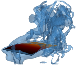
In figure 8, we show surfaces of constant vorticity magnitude generated at resonance by externally and internally actuated plates as predicted by our simulations. Vorticity is generated as a result of the relative motion of the plate with respect to the surrounding fluid and, therefore, is the most significant along the trailing edge (TEVs) and the side edges (SEVs) of the plate. During each stroke the combination of SEVs and TEVs forms a characteristic horseshoe shaped set of vortices that are periodically shed from the oscillating plate. The horseshoe vortices sharing common features are generated by plates with both modes of actuation. However, there are also important differences in the emerging flow structures associated with their distinct bending patterns.

Figure 8. Contours of normalized vorticity  $\omega \tau = \pm 10$ of the numerically simulated (a–d) externally actuated plate and (e–h) internally actuated plate with
  $\mathcal {A}_{\mathcal {R}} = 2$,
  $\chi = 5$,
  $Re = 1000$, and tip deflection
  $\delta _t/L = 0.25$ at resonance at times
  $t/\tau = 0.25$, 0.5, 0.75, 1, respectively. Vortices represented in red are rotating anticlockwise while vortices represented in blue are rotating clockwise.
Several theoretical and experimental studies highlight the key role of reverse Kármán streets for propulsion (Nauen & Lauder Reference Nauen and Lauder2002; Alben Reference Alben2009; Michelin & Llewellyn Smith Reference Michelin and Llewellyn Smith2009). Both actuation patterns lead to the generation of sets of vortices with opposite rotation direction. In both instances, anticlockwise vortices are shed at the top while clockwise rotating vortices are shed at the bottom. The direction of these vortices creates a jet flowing away from the tip of the plate. This configuration leads to the production of a net thrust. For the lowest actuation levels tested, the sign of these vortices flip which corresponds to a net drag force on the plate (Anderson et al. Reference Anderson, Streitlien, Barrett and Triantafyllou1998; Nauen & Lauder Reference Nauen and Lauder2002; Alben Reference Alben2009; Michelin & Llewellyn Smith Reference Michelin and Llewellyn Smith2009; Paraz et al. Reference Paraz, Schouveiler and Eloy2016).
When considering the external actuation, the plunging motion of the plate leading edge produces a leading edge vortex (LEV), however, its strength is relatively weak compared with SEVs and TEV. Since the plate is actuated in a quiescent fluid, the LEVs shed close to the root and do not interact in the wake with TEVs and SEVs. Therefore, we do not anticipate they play an important role in the thrust production for this set-up. Furthermore, SEVs extend along the entire plate length from the root to the tip. In the case of the internal actuation, the root is immobilized. As a result, the internally actuated plate does not produce LEVs, whereas significant SEVs develop only at a halfway distance from the root to the tip. Thus, one can expect the externally actuated plate that displaces more fluid during each stroke would generate more vorticity compared with the internally actuated plate with comparable trailing edge displacement.
To further characterize the flow field, figure 9 shows simulation snapshots of the flow field around oscillating plates with different actuation types. The glyph demonstrates the alternating vortical structure shed at the tip of the plate. A downstroke generates anticlockwise vortices, as shown in figures 9(b), 9(c), 9(f) and 9(g), whereas the upstroke generates clockwise vortices, as shown in figures 9(a), 9(d), 9(e) and 9(h) (see also supplementary material available at https://doi.org/10.1017/jfm.2020.915). The interaction of the vortices creates a jet in the  $x$-direction leading to a net thrust. We note that these flow structures are consistent with the literature (Facci & Porfiri Reference Facci and Porfiri2013).

Figure 9. Normalized velocity magnitude  $\vert \vert \boldsymbol{U} \vert \vert / U_0$ of the numerically simulated (a–d) externally and (e–h) internally actuated plate with
  $\mathcal {A}_{\mathcal {R}} = 2$,
  $\chi = 5$,
  $Re = 1000$, and tip deflection
  $\delta _t/L = 0.25$ at resonance at times (a–d)
  $t/\tau = 0.25, 0.5, 0.75, 1$, respectively.
We quantified the vorticity generated by each actuation method by computing the normalized enstrophy  $\mathcal {E} = \boldsymbol {\omega } \boldsymbol{\cdot} \boldsymbol {\omega } \, \tau ^{2}$. Enstrophy is a measure of the intensity of viscous dissipation (Weiss Reference Weiss1991). In figure 10, we show the time evolution of the volume-averaged enstrophy over one period of plate oscillations. For both plates the enstrophy displays similar time-dependent behaviour with two peaks. However, the locations of the peaks are somewhat different. Compared with the plates with external actuation, the peaks for the internally actuated plate shifted towards the ends of the upstroke and the downstroke at
  $t/\tau = 0.2$ and
  $t/\tau = 0.7$, respectively. Figure 10 also shows that throughout most of the oscillation period, the internally actuated plate generates noticeable greater enstrophy and, therefore, viscous dissipation compared with the externally actuated plate.

Figure 10. Time history of the normalized bulk enstrophy  $\mathcal {E}_{bulk}$ for numerically simulated internally and externally actuated plates with
  $\mathcal {A}_{\mathcal {R}} = 2$,
  $\chi = 5$,
  $Re = 1000$, and tip deflection
  $\delta _t/L = 0.25$ at resonance.
We find that, for the externally actuated plate, the maximum viscous dissipation coincides with the maximum tip deflection, whereas the minimum enstrophy corresponds to zero tip deflection (figure 7a). In the case of the internally actuated plate, however, enstrophy production is related to the plate curvature at the trailing edge. Indeed, comparing figures 7(c) and 10, we find that the maxima of enstrophy are close to the maxima of tip curvature at  $t/\tau = 0.25$ and
  $t/\tau = 0.75$, while the enstrophy minima coincide with zero tip curvature at
  $t/\tau = 0.5$ and
  $t/\tau = 1$. Thus, the ‘cupping’ exhibited by the internally actuated plate is a major contributor causing the increased enstrophy production and, therefore, viscous dissipation.
5.3. Hydrodynamic forces
To further investigate the difference between the two actuation methods, we examine time evolution of the hydrodynamic force generated by the plates. In figure 11(a), we show the simulation results for the instantaneous lift force  $F_z$ over one oscillation period. The input refers to the prescribed motion at the root and the internal moment for the externally and internally actuated plates, respectively. We normalize the forces by the characteristic force based on the plate length. The externally and internally actuated plates yield comparable maximum lift. The maximum occurs close to
  ${\rm \pi} /2$ coinciding with the phase of the maximum plate displacement at resonance. The mean lift force is zero due to the symmetry of the periodic oscillations.

Figure 11. Time histories of (a) the lift force and (b) the thrust force for numerically simulated internally and externally actuated plates with  $\mathcal {A}_{\mathcal {R}} = 2$,
  $\chi = 5$,
  $Re = 1000$ and tip displacement
  $\delta _t/L = 0.25$ at resonance. The horizontal dotted lines show the mean values of the thrust force.
The thrust force  $F_x$ generated by the plates is presented in figure 11(b). The peak-to-peak amplitude of the thrust force is similar for both cases. The difference is, however, that the externally actuated plate generates a significantly greater period-averaged thrust compared with the internally actuated plate. The figure shows that there is almost a twofold difference in the value of the net thrust between the externally and internally plates. We relate this difference to the bending patterns shown in figure 6, where the negative angle at the tip or ‘cupping’ of the internally actuated plate yields a plate shape that is ineffective for propelling fluid backwards. Thus, the externally actuated plate yields substantially greater thrust than the internally actuated plate with the same tip displacement.
In figure 12(a), we plot the dependence of the mean thrust force on the tip deflection  $\delta _t$ for the externally and internally actuated plates with two different aspect ratios. Overall, the normalized thrust increases with the tip deflection. For relatively small
  $\delta _t/L$ (up to approximately 0.05) that roughly corresponds to the linear regime of the plate oscillations, the increase is almost linear with
  $\delta _t$ (see inset in figure 12a). For larger values of
  $\delta _t$, the thrust scales as
  $\delta _t^{3}$ indicating the influence of the nonlinear effects. For the two aspect ratios tested, the externally actuated plates generate greater thrust compared with the internally actuated plates. This suggests that externally actuated plates outperform internally actuated plates independently of the aspect ratio given that they have similar trailing edge displacements.

Figure 12. Dependence of (a) the normalized thrust  $F_x/F_0$, (b) input power
  $\mathcal {P}/P_0$ and (c) efficiency
  $\eta$ on the tip deflection magnitude
  $\delta _t$. The simulation results are for
  $Re = 1000$,
  $\chi = 5$ and two aspect ratios
  $\mathcal {A}_{\mathcal {R}} = 2$ and
  $\mathcal {A}_{\mathcal {R}} = 4$.
Furthermore, for both the external and internal actuation methods, we find that wider plates with  $\mathcal {A}_{\mathcal {R}} = 2$ produce greater thrust than more narrow plates with
  $\mathcal {A}_{\mathcal {R}} = 4$. This difference can be attributed to the effect of SEVs (Raspa et al. Reference Raspa, Ramananarivo, Thiria and Godoy-Diana2014; Yeh & Alexeev Reference Yeh and Alexeev2016b). It was shown using scaling arguments that SEVs increase with the tip displacement, but not the plate width. Therefore, for the same tip displacement a wider plate experiences a weaker adverse effect of SEVs and generates more thrust per plate unit width.
The power consumption by the internally and externally actuated plates is shown in figure 12(b) as a function of the tip deflection  $\delta _t$. The power input increases monotonically with the tip deflection for both actuation methods. For small deflection amplitudes
  $\delta _t/L<0.05$, the power
  $\mathcal {P}$ increases proportionally to
  $\delta _t^{2}$, whereas for larger
  $\delta _t$, the power increases as
  $\delta _t^{3}$ (see inset in figure 12b). We find that the wider plates require greater power input per unit width compared with the narrow plates independently of the actuation method. This is consistent with the higher thrust produced by the wider plates (figure 12a) and can be related to larger amounts of fluid displaced by such plates per unit width. Furthermore, we find that externally actuated plates require greater input power to oscillate with the same tip deflection as internally actuated plates. This can be in part attributed to the additional power required by an externally actuated plate to displace fluid near the oscillating plate root compared with the internally actuated plate with clamped root. Indeed, even at small levels of actuation the LEVs and SEVs have comparable sizes (figure 8).
To further characterize the hydrodynamic performance of oscillating plates, we compute the thrust efficiency  $\eta = {F_x/F_0}/{\mathcal {P}/P_0}$ in figure 12(c) as a function
  $\delta _t$. We find that the efficiency is maximized for smaller
  $\delta _t$, but rapidly decreases with increasing
  $\delta _t$ within the linear regime. In the nonlinear regime, the efficiency varies slightly with
  $\delta _t$. Indeed, in the linear regime
  $F_x \sim \delta _t$ and
  $\mathcal {P} \sim \delta _t^{2}$ resulting in
  $\eta \sim 1/\delta _t$. For greater
  $\delta _t$ characterized by nonlinear oscillations, both
  $F_x$ and
  $\mathcal {P}$ scale with
  $\delta _t^{3}$, which in turn results in
  $\eta$ nearly independent of
  $\delta _t$. Comparing the externally and internally actuated plates, we find that the externally actuated plates exhibit higher efficiency than the internally actuated plates, except for the lowest tip deflection conditions. This is because at small
  $\delta _t$ the efficiency of the externally actuated plate is reduced due to the plunging motion at the root that dissipates energy but does not contribute to the thrust. For larger values of
  $\delta _t$, externally actuated plates outperform internally actuated plates with the same aspect ratio. The reduced efficiency of internally actuated plates is associated with the trailing edge curvature disrupting the flow and generating an increased level of vorticity, as shown in figure 10. We also find that wider plates are more efficient than narrow plates for the entire range of
  $\delta _t$. This is due to the lower contribution of SEVs into the overall energy budget of the wider plates.
In figure 13, we use simulations to probe the effect of the flow regime by varying the Reynolds number for the two actuation methods. Here, we consider plates with two values of tip deflections and  $\mathcal {A}_{\mathcal {R}} = 2$. In figure 13(a), we show that the normalized thrust does not change significantly with
  $Re$. As demonstrated by Lighthill (Reference Lighthill1970), at high enough
  $Re$ the thrust is mainly defined by the tip kinematics, supported by nearly constant thrust for higher
  $Re$. Conversely at lower
  $Re$, the tip kinematics do not fully define the thrust production. This trend persists for both types of actuation, although the externally actuated plates produce greater thrust.

Figure 13. Dependence of (a) the normalized thrust  $F_x/F_0$, (b) input power
  $\mathcal {P}/P_0$ and (c) efficiency
  $\eta$ on the Reynolds number,
  $Re$. The simulation results are for
  $\delta _t/L = 0.15$,
  $\delta _t/L = 0.25$,
  $\chi = 5$ and
  $\mathcal {A}_{\mathcal {R}} = 2$.
In figure 13(b), we show the evolution of the normalized power with  $Re$. As the Reynolds number increases the normalized power decreases and remains constant at higher
  $Re$. This behaviour can be attributed to the increase of viscous dissipation associated with a lower
  $Re$. To generate the same tip deflection, the plate requires more power when the viscous effects are more significant. For both tested tip deflections, the internally actuated plates consume less power compared with the externally actuated plates.
The change of the hydrodynamic efficiency of the plates with  $Re$ is shown in figure 13(c). Over the entire range of
  $Re$ we tested, the externally actuated plates outperform the internally actuated plates. The difference in efficiency is more significant for the lower tip deflection amplitude. This indicates that as the viscous effects become more important, the hydrodynamic efficiency is more sensitive to the difference in bending patterns of the internally and externally actuated plates. Conversely, at higher Reynolds number, the hydrodynamic efficiency converges to a constant value. This behaviour is consistent with the potential flow solution predicting that the efficiency is set by the tip kinematics.
In figures 14(a) and 14(b), we show the inertia coefficient  $c_m$ for plates with, respectively,
  $\mathcal {A}_{\mathcal {R}} = 2$ and
  $\mathcal {A}_{\mathcal {R}} = 4$ as a function of the tip deflection
  $\delta _t$. We find close agreement between the experiments and simulations despite that they use different values of the mass ratio
  $\chi$. As shown in the inset in figure 14(a), the inertia coefficient is nearly independent of
  $\chi$ for
  $\chi > 2.5$. This explains good agreement between simulations and experiments in figures 14(a) and 14(b), where the simulations are performed with
  $\chi = 5$, whereas the experimental plates are, respectively, characterized by
  $\chi = 20$ and
  $\chi = 10$.

Figure 14. Dependence of inertia mass coefficient on the tip deflection in the linear oscillation regime of internally and externally actuated plates for  $Re = 1000$,
  $\chi = 5$ and aspect ratios (a)
  $\mathcal {A}_{\mathcal {R}} = 2$ and (b)
  $\mathcal {A}_{\mathcal {R}} = 4$. (c) Dependence of the inertia mass coefficient on
  $Re$ for
  $\mathcal {A}_{\mathcal {R}} = 2$,
  $\chi = 5$,
  $\delta _t/L = 0.05$ and
  $\delta _t/L=0.25$. The left-hand inset in (a) shows the dependence of the inertia coefficient on the mass ratio for
  $\delta _t/L = 0.01$. The right-hand inset in panel (a) and inset in panel (b) show the inertia coefficient for nonlinear range of plate oscillations. In panels (a,b) the lines represent simulation results while the symbols represent experimental data, whereas panel (c) is simulation results only.
Our experiments are limited to relatively small tip deflections, approximately  $\delta _t = 0.05$. In the simulations, we explore a significantly wider range of
  $\delta _t$, shown in the insets in figures 14(a) and 14(b). We find that the inertia coefficient plateaus with the increasing tip deflection, consistent for both types of actuation. Although it can be expected that the inertia coefficient is a sole function of the aspect ratio and the tip amplitude, our results show that the actuation method strongly affects
  $c_m$. Not only does
  $c_m$ increase with the tip amplitude, but also the difference between
  $c_m$ for two actuation methods increases with
  $\delta _t$. For larger
  $\delta _t$, the inertia coefficient for the externally actuated plate systematically exceeds
  $c_m$ of the internally actuated plate. This result is in agreement with the hydrodynamic loading acting on the plate shown in figure 12. The externally actuated plate produces greater hydrodynamic forces and, therefore, is characterized by a higher inertia coefficient than the internally actuated plate.
In figure 14(c), we show simulation results for the inertia coefficient as a function of  $Re$. The simulations are performed for externally and internally actuated plates with two values of the tip deflection. We find that
  $c_m$ gradually decreases with
  $Re$. This result agrees with the theory (Van Eysden & Sader Reference Van Eysden and Sader2006, Reference Van Eysden and Sader2007; Tuck Reference Tuck1969) suggesting that as the viscous effects lessen and inertia dominates the inertia coefficient asymptotically converges to 1. Thus, at sufficiently high
  $Re$ the added mass effect saturates and is nearly independent of the actuation method.
6. Conclusion
We systematically investigate and compare the hydrodynamics of elastic plates oscillating in an incompressible Newtonian fluid subjected to two distinct actuation methods. We probe the resonance oscillations in linear and nonlinear regimes of an externally actuated plate and a plate with an internal actuation. We pinpoint the critical differences in their bending patterns leading to different hydrodynamics performances. Specifically, the internally actuated plates display ‘cupping’ of the trailing edge due to a non-zero plate curvature induced by the internal bending moment. Furthermore, internally actuated plates exhibit a phase change of the plate angle along the plate length. Conversely, externally actuated plates have a zero curvature at the tip and an in-phase plate angle along the entire plate length. We show that this difference in bending pattern between internally and externally actuated plates leads to greater vorticity production by internally actuated plates and therefore enhances the viscous dissipation.
We find that for the same level of trailing edge displacement externally actuated plates outperform internally actuated plates in terms of the generated thrust and consumed power. Furthermore, plates with external actuation are more efficient than plates with internal actuation with the exception of the smaller tip amplitudes, in which the efficiency of the externally actuated plates is limited due to the root displacement. For both actuation methods, we find that wider plates outperform more narrow plates due to the adverse effects of the side edge vortexes. Additionally, we also probe the effect of the actuation method on the plate inertia coefficient and find that the inertia coefficient is insensitive to the mass ratio for ratios greater than 2.5. In the linear oscillation regime, both actuation methods are characterized by similar values of the inertia coefficient. However, for larger tip deflections, the inertia coefficient of the externally actuated plate significantly exceeds that of internally actuated plates, which is related to the greater hydrodynamic forces experienced by the externally actuated plates. Thus we show that the inertia coefficient is not only a function of the aspect ratio and tip deflection, but also the actuation pattern.
We show that in the range  $500<Re<4000$, the Reynolds number has minor influence on the thrust generated by the plate. We find that the plate kinematics defining the thrust production does not change significantly in this
  $Re$ range. Conversely,
  $Re$ impacts the power and, therefore, hydrodynamic efficiency of the plate. At lower
  $Re$, viscous effects increase the input power that, in turn, negatively affects the efficiency. Increasing
  $Re$ also leads to a decrease of the inertia coefficient that converges to unity for higher
  $Re$. This behaviour is consistent with the analytical solution for an inviscid fluid. We find that these trends prevail for both actuation methods. Nevertheless, for lower
  $Re$ the dependence of the plate hydrodynamics on the actuation method is more critical.
The results of our study provide useful guidelines for designing efficient biomimetic underwater robotic vehicles that utilize internally actuated propulsors such as piezoelectric actuators. Piezoelectric actuators are highly attractive due to a high degree of control over the bending pattern including a combined twisting–bending motion, large amplitude actuation, silent operation and the ease of interaction into robotic swimmers. Our study points to the need for improving the efficiency of internally actuated propulsors to match or exceed the efficiency achievable with externally actuated elastic fins. Different strategies can be explored to enhance the efficiency of piezoelectric propulsors including the use of passive attachments (Yeh & Alexeev Reference Yeh and Alexeev2016a), complex actuation cycles and a combination of an external and internal actuation. These studies are currently underway. Furthermore, the results of this work are useful for developing piezoelectric energy harvesting devices. In the latter scenario, fluid motion is harnessed to include oscillations of elastic structures with embedded piezoelectric transducers.
Acknowledgements
We thank the National Science Foundation (CBET-1705739) for financial support. The work used the Extreme Science and Engineering Discovery Environment (XSEDE) provided through Award TG-DMR180038.
Declaration of interests
The authors report no conflict of interest.
Supplementary material and movies
Supplementary material and movies are available at https://doi.org/10.1017/jfm.2020.915.
Appendix A. Inertia coefficient
We can rewrite (2.2) with an additional mass per area  $\mathcal {M}$ as
 \begin{equation} \omega_{1,{f}}= \frac{\lambda^{2}_1}{L^{2}} \sqrt{\frac{D}{\sigma_s + \mathcal{M}}} {.} \end{equation}
By comparing the two definitions, we can obtain
 \begin{equation} \frac{\omega^{2}_{1,{vac}}}{\omega^{2}_{1,{f}}} = 1+{\frac{\mathcal{M}}{\sigma_s}} {.} \end{equation}
 For plates with moderate and high aspect ratios, the added mass can be expressed as  $\mathcal {M} = ({{\rm \pi} }/{4} )\rho W c_m = ({{\rm \pi} }/{4}) \chi \sigma _s c_m$, with
  $c_m$ being the inertia coefficient. We therefore evaluate the inertia coefficient as follows:
 \begin{equation} c_m = \frac{4}{{\rm \pi} \chi}\left(\frac{\omega^{2}_{1,{vac}}}{\omega^{2}_{1,\text{f}}}-1\right) {.} \end{equation}
Appendix B. Discretization
In discretized form (with  $\gamma = 0$), (3.9) yields
 \begin{align} &\frac{\rho h}{{\rm \Delta} t^{2}} \left(w_{i,j}^{n+1}-2w_{i,j}^{n}+w_{i,j}^{n-1}\right) \nonumber\\ &\quad = q_{i,j}^{n} + w_{i+2,j}^{n} \left(\frac{-D}{{\rm \Delta} x^{4}}\right) + w_{i-2,j}^{n} \left(\frac{-D}{{\rm \Delta} x^{4}}\right) + w_{i,j+2}^{n} \left(\frac{-D}{{\rm \Delta} y^{4}}\right) + w_{i,j-2}^{n} \left(\frac{-D}{{\rm \Delta} y^{4}}\right)\nonumber\\ &\qquad+ w_{i+1,j+1}^{n} \left(-\frac{2D}{{\rm \Delta} x^{2} {\rm \Delta} y^{2}} + \frac{N_{xy i,j}^{n}}{4{\rm \Delta} x {\rm \Delta} y} \right) + w_{i-1,j+1}^{n} \left(-\frac{2D}{{\rm \Delta} x^{2} {\rm \Delta} y^{2}} - \frac{N_{xy i,j}^{n}}{4{\rm \Delta} x {\rm \Delta} y} \right)\nonumber\\ &\qquad + w_{i+1,j-1}^{n} \left(-\frac{2D}{{\rm \Delta} x^{2} {\rm \Delta} y^{2}} - \frac{N_{xy i,j}^{n}}{4{\rm \Delta} x {\rm \Delta} y} \right) + w_{i-1,j-1}^{n} \left(-\frac{2D}{{\rm \Delta} x^{2} {\rm \Delta} y^{2}} + \frac{N_{xy i,j}^{n}}{4{\rm \Delta} x {\rm \Delta} y} \right)\nonumber\\ &\qquad + w_{i,j}^{n} \left[-D\left(\frac{6}{{\rm \Delta} x^{4}}+\frac{8}{{\rm \Delta} x^{2} {\rm \Delta} y^{2}}+\frac{6}{{\rm \Delta} y^{4}}\right) -\frac{2 N_{x i,j}^{n}}{{\rm \Delta} x^{2}} -\frac{2 N_{y i,j}^{n}}{{\rm \Delta} y^{2}} \right] \nonumber\\ &\qquad + w_{i+1,j}^{n} \left[4 D \left(\frac{1}{{\rm \Delta} x^{4}}+\frac{1}{{\rm \Delta} x^{2} {\rm \Delta} y ^{2}}\right) + \frac{N_{x i,j}^{n}}{{\rm \Delta} x^{2}} \right]\nonumber\\ &\qquad + w_{i-1,j}^{n} \left[4 D \left(\frac{1}{{\rm \Delta} x^{4}}+\frac{1}{{\rm \Delta} x^{2} {\rm \Delta} y ^{2}} \right) + \frac{N_{x i,j}^{n}}{{\rm \Delta} x^{2}}\right]\nonumber\\ &\qquad + w_{i,j+1}^{n} \left[4 D \left(\frac{1}{{\rm \Delta} y^{4}}+\frac{1}{{\rm \Delta} x^{2} {\rm \Delta} y ^{2}}\right) + \frac{N_{y i,j}^{n}}{{\rm \Delta} y^{2}} \right] \nonumber\\ &\qquad + w_{i,j-1}^{n} \left[4 D \left(\frac{1}{{\rm \Delta} y^{4}}+\frac{1}{{\rm \Delta} x^{2} {\rm \Delta} y ^{2}}\right) + \frac{N_{y i,j}^{n}}{{\rm \Delta} y^{2}}\right] . \end{align}
 To constrain plate stretching during the deformation we impose the inextensibility condition. This condition is enforced numerically by introducing a differential arclength  $\textrm {d}s^{2} = {\textrm {d} x}^{2} + \textrm {d}w^{2}$ that is numerically approximated as
 \begin{equation} x_{i+1} = x_i + \sqrt{{\rm \Delta} s^{2} - \left(w_{i+1}-w_i\right)^{2}} . \end{equation}


