


1 Introduction
When decision makers choose between two alternatives A and B, the availability of a third alternative Z that they judge to be clearly inferior to A but not to B tends to increase their preference for A. For example, a decision maker wanting to buy an office printer may feel indifferent between a printer A, costing $200 with replacement cartridges that cost $50 each, and another B, costing $100 with replacement cartridges that cost $70 each; but the availability of a third option Z, costing $220 with replacement cartridges that cost $60 each, may cause the decision maker to prefer A to B, because A is cheaper than Z on both relevant product attributes, whereas B is not. This phenomenon was first discovered in individual decision making by Huber et al. (Reference Huber, Payne and Puto1982) and is called the asymmetric dominance effect (ADE), decoy effect, or attraction effect (e.g., Chang et al., Reference Chang, Chang and Liao2015; Sürücü et al., Reference Sürücü, Djawadi and Recker2019). In general, the asymmetric dominance effect is an increase in preference for an option A relative to another option B caused by its dominance over an irrelevant option Z, whether or not A and B are initially equally preferred. It yields substantial effect sizes and has been shown to occur not only under experimental conditions but also in real in-store and online purchases, even when the asymmetrically dominated alternative Z is presented as an unavailable phantom decoy option, like an item in a shopping catalogue marked “out of stock” and therefore visible but unavailable for choice (Ariely & Wallsten, Reference Ariely and Wallsten1995; Doyle et al., Reference Doyle, O’Connor, Reynolds and Bottomley1999; Huber et al., Reference Huber, Payne and Puto2014).
Colman et al. (Reference Colman, Pulford and Bolger2007) discovered an equivalent effect in interactive decision making, when a player's strategy A, but not another strategy B, strictly dominates a third strategy Z, and they called this the strategic asymmetric dominance effect. Such an effect can occur in any social interaction in which the strategic structure involves an asymmetrically dominated strategy. A comparison of players’ one-off (unrepeated) choices in 18 different 3 × 3 experimental games with asymmetrically dominated strategies, and choices in a control condition of one-off choices in 2 × 2 versions of the same games with the asymmetrically dominated strategies removed, revealed that players chose the asymmetric dominant strategies in the 3 × 3 games significantly more frequently than the corresponding strategies in the 2 × 2 control games. The presence of asymmetrically dominated strategies in the experimental games, even when they were visible but unavailable for choice in a phantom decoy treatment condition, increased choices of the strategies that dominated them. These findings were confirmed by Galeotti et al. (Reference Galeotti, Montero and Poulsen2022), who reported significant strategic asymmetric dominance effects in two experiments in which players negotiated over pairs and triplets of options defined solely by the sizes of the players’ payoffs.
From a theoretical perspective, the asymmetric dominance effect (whether in individual or interactive decision making) is clearly irrational. It violates a basic contraction property of rational choice called Property α (Sen, Reference Sen1969), according to which, for example, if the oldest person in the world happens to live in France, then that person must also be the oldest person in France. In formal logic, if xRy is a binary relation denoting weak preference for x over y, we can define a choice function c that assigns a choice set C(Y, R) to every non-empty feasible subset Y of X, such that [x ∈ C(Y, R) ⇔ xRy], for all y ∈ Y, where Y is the feasible subset of the universal set X. Then, we have:
 $$\eqalign{& {\rm{Property}}\,{\rm{\alpha: = }}\,{\rm{[[}}x \in {\rm{C}}\left( {X{\rm{,}}R} \right) \wedge x \in Y \subseteq X{\rm{]}} \Rightarrow x \in C\left( {Y{\rm{,}}R} \right){\rm{],}} \cr & {\rm{for}}\,{\rm{all}}\,x \in C\left( {X{\rm{,}}R} \right) \cr} $$
Property α is a special case of a fundamental axiom of decision theory called Condition IIa (Nash, Reference Nash1950) or more commonly the independence of irrelevant alternatives (Chernoff, Reference Chernoff1954), according to which an individual's preference between alternatives A and B should never be affected by the presence or absence of a third alternative Z. The following example, adapted from Luce and Raiffa (Reference Luce and Raiffa1957, p. 288), provides an illustration of this principle in everyday decision making, not necessarily related to asymmetric dominance in particular. Suppose a customer in a restaurant examines the menu, whittles the choice down to either pasta bake or mushroom risotto, and finally decides to order the pasta bake in preference to the mushroom risotto. The waiter then announces that a special seafood dish, not on the menu, is also available. The customer, who dislikes seafood, responds: “Oh well, in that case I’d prefer the mushroom risotto to the pasta bake.” The customer has violated both Property α and the independence of irrelevant alternatives: the addition of the seafood dish to the menu should be irrelevant to the customer's preference between pasta bake and mushroom risotto.
The asymmetric dominance effect is a specific type of violation of the independence of irrelevant alternatives and is thus fundamentally irrational. In everyday life, individual and interactive choices are often repeated rather than just one-off decisions, thus it is important to know whether asymmetric dominance effects persist or decay over time when decisions involving asymmetric dominance are repeated. The asymmetric dominance effect is clearly a special kind of context effect, because, like any other context effect, it is a distortion of judgment arising from the presence of a distracting and irrelevant contextual element in a mental representation. This immediately suggests comparison with associative visual illusions in psychology, where perception is similarly distorted by context effects involving distracting elements of visual images. This may at first seem a far-fetched connection, but Trueblood et al. (Reference Trueblood, Brown, Heathcote and Busemeyer2013) and Trueblood (Reference Trueblood2022) have argued persuasively for a unified theoretical account of context effects in decision making and perceptual phenomena. Indirect evidence that the asymmetric dominance effect could itself be a perceptual phenomenon rather than requiring value-based reasoning involving formal argumentation (Bench-Capon et al., Reference Bench-Capon, Atkinson and McBurney2012) comes from the discovery that honeybees and grey jays are susceptible to asymmetric dominance effects (Shafir et al., Reference Shafir, Waite and Smith2002). Even if it is not strictly perceptual, the asymmetric dominance effect may not fully engage value-based decision making. For an investigation and discussion of perceptual and value-based decisions, see Trueblood and Pettibone (Reference Trueblood and Pettibone2017).
1.1 Theoretical considerations and previous findings
Investigations of associative visual illusions, such as the familiar Müller–Lyer illusion (for an illustration, see https://how-emotions-are-made.com/notes/M%C3%BCller-Lyer_illusion), have revealed that they manifest what is called illusion decrement under repetition or prolonged inspection (Köhler & Fishback, Reference Köhler and Fishback1950; Predebon, Reference Predebon2006; Predebon et al., Reference Predebon, Stevens and Petocz1993). However, there are other types of visual illusions, such as the less familiar leaning tower illusion (illustrated at https://illusionoftheyear.com/2007/05/the-leaning-tower-illusion), that seem to persist indefinitely without decrement (Kingdom et al., Reference Kingdom, Yoonessi and Gheorghiu2007a, Reference Kingdom, Yoonessi and Gheorghiub, Reference Kingdom, Yoonessi, Gheorghiu, Shapiro and Todorovic2017).
For theoretical reasons, we might expect the asymmetric dominance effect to decrease over repetitions, because it seems more similar to the Müller–Lyer illusion, arising as it does from a context-effect bias in information processing. The Müller–Lyer illusion, like any associative visual illusion, results from part of an image causing a bias in perception of another part, whereas the leaning tower illusion is a perspective illusion, resulting from a natural visual process operating normally from an incorrect starting assumption. In the leaning tower illusion, our visual system misinterprets a pair of images as parts of a single image, and for some reason we find it difficult to discount this assumption even when we know it to be false. In a single image of a pair of towers photographed from below, with the camera tilted upward, linear perspective would cause the towers to converge toward the top of the image. In the unnatural double image used in the illusion, this perspective convergence is missing, and the towers therefore appear to diverge, although they are actually parallel: the effect arises from a natural visual process working normally on the basis of a false assumption. The Müller–Lyer illusion, like the asymmetric dominance effect, appears to result from a pure context effect. A further more general reason to expect repetition-induced decrement in the strategic asymmetric dominance effect, in particular, is experimental evidence from other types of games (e.g., Parco et al., Reference Parco, Rapoport and Stein2002; Slonim & Roth, Reference Slonim and Roth1998) in which players generally tend to converge toward more rational choices over repetitions.
On the other hand, experiments have yielded mixed results regarding repetition-induced decrement of the asymmetric dominance effect, although published evidence is sparse for the individual-choice asymmetric dominance effect and almost non-existent for the strategic asymmetric dominance effect. Turning first to the effects of repetition on the asymmetric dominance effect in individual decisions, Ahn et al. (Reference Ahn, Kim and Ha2015) reported two experiments in which participants attempted to choose the best rafting boats from choice sets including asymmetrically dominated options, with or without expert feedback after every trial. In the first experiment, repeated over 10 trials, the choice sets contained either two or three options, and in the second experiment, repeated over 45 trials, the choice sets contained either three or four options. In both experiments, asymmetrically dominated options were included in the larger choice sets, and choices of the options that dominated them were compared with choices of the same options in the smaller choice sets without the dominated options. The results revealed that asymmetric dominance occurred in both experiments, and repetition weakened the effect significantly, with or without expert feedback in the first experiment, and only with expert feedback in the more complex second experiment.
Crosetto and Gaudeul (Reference Crosetto and Gaudeul2023) reported data from a process-tracing study of individual decisions involving the asymmetric dominance effect. This study discovered what turned out to be rapid decrement over time in the effect while decision makers were contemplating particular decisions. This study used an intuitive and incentive-compatible task to investigate decision making over 40 repetitions but did not report or attempt to investigate the effects of repetition per se: instead, the researchers focused attention on temporal effects within individual decisions. Participants received a fixed budget per round to select the cheapest option for buying gasoline from pairs or triplets of options, keeping any unspent money for themselves. Each option was displayed only as a quantity and a price for that quantity—for example, 1.6 L costing €2.11—making it difficult for the participants to calculate the price per liter in order to compare it with other options and to choose the cheapest one, thereby earning the maximum payoffs for themselves. The options were combined randomly so that only some triplets included an asymmetrically dominated option—with both a greater quantity and a cheaper price per liter than another option within the same triplet. Participants had 20 s to record their decisions via computers and were free to change their minds as frequently as they wished during that time. From the recorded data the researchers were able to track the participants’ judgments over time, and the results revealed that the asymmetric dominance effect “is not a persistent feature of choice but rather a temporary [short-lasting] heuristic that drives choice in the first seconds of exposure to stimuli but largely disappears in the long run” (p. 23).
As far as we are aware, only two published studies have attempted to examine the effects of repetition on the strategic asymmetric dominance effect in interactive decisions—decisions involving at least two decision makers whose outcomes depend not only on their own choice but also on those of the other player. First, Amaldoss et al. (Reference Amaldoss, Bettman and Payne2008, Study 2) investigated the effect of adding an asymmetrically but weakly dominated third strategy to the row player's strategy set only in several versions of the 2 × 2 Leader game, repeated over 40 rounds with outcome feedback after every round. In the Leader game, neither player has a dominant strategy, but there are two pure-strategy Nash equilibria, one preferred by the row player and the other preferred by the column player. When the asymmetrically dominated strategy was absent, players failed to coordinate on either equilibrium, but when it was present, row players tended over repeated rounds to move toward the equilibrium associated with the asymmetrically dominant strategy from their point of view, but column players showed no evidence of adjusting their own strategy choices accordingly. The researchers were principally concerned with equilibrium selection, but they commented, in an aside: “The asymmetric dominance effect did not wear out over the several replications of the game. On the contrary, the effect grew in strength” (p. 912). However, asymmetric dominance is usually understood to involve a strictly dominated option, therefore this study leaves open the question as to the effect of repetition on the strategic asymmetric dominance effect in its true form.
The only other attempt to investigate the effect of repetition on the strategic asymmetric dominance effect appears to be a study of Wang et al. (Reference Wang, Jusup, Shi, Lee, Iwasa and Boccaletti2018). The experimental game used in this study was a conventional Prisoner's Dilemma game, with strategies labeled C and D, plus an additional strategy R for each player, strictly dominated by both C and D. The intention was to “focus on the decoy effect, also known as the asymmetric dominance effect” (p. 2). However, the appended strategy R was not asymmetrically dominated (by one other strategy) but symmetrically dominated (by both other strategies), and the findings, interesting though they are, do not seem to relate to asymmetric dominance as it is normally understood. No significant trend in cooperative choices occurred—no increase or decrease of C choices—over 80 repetitions of the game, with or without the additional R strategies, but when the R strategies were present, C choices were significantly more frequent across the 80 repetitions than when it was absent. The Prisoner's Dilemma seems an unfortunate choice for this experiment, because the C strategy is strictly dominated by the D strategy even without the additional R strategy. A further unusual feature of the experiment was the fact that the time series of 80 repetitions comprised sub-sequences of “infinite-horizon” games in which there was a fixed probability of a sequence of repetitions ending randomly after every round. Players were paired to play with a 0.25 probability of the sequence ending after every round and were thus paired with a different co-player after every four rounds, on average, until 80 rounds had been completed. Psychologically, this is likely to have been experienced as a succession of 20 four-round interactions with different co-players, rather than 80 repetitions. Changes of co-players in repeated Prisoner's Dilemma games have been shown to generate quasi-endgame effects (Colman et al., Reference Colman, Pulford and Krockow2018), causing players to reset their levels of cooperation after each change and damping longer-term trends. Wang et al.'s time series does in fact show such short-run fluctuations, on which they comment: “The negative value of β 3 [an autoregression parameter] reflects a self-correcting nature (i.e., stationarity) of the examined time series” (p. 3), but these fluctuations may in fact represent quasi-endgame effects, repeatedly resetting cooperation levels and thereby blocking the decline in C choosing that would otherwise occur.
2 The present experiment
The experiment reported in this article is, as far as we are aware, the first to investigate the effects of repetition on the strategic asymmetric dominance effect in its true form—in 3 × 3 games with one strategy strictly dominated by just one other for each player and no other dominance relations between strategies. We examine the effect over 50 repetitions, with outcome feedback after each repetition, in fixed player pairs. The three experimental games used were selected from a static (one-shot) asymmetric dominance experiment of Colman et al. (Reference Colman, Pulford and Bolger2007) in which the effect was first reported. The basic comparison is between choices in 2 × 2 games without dominant strategies and choices in 3 × 3 games constructed by appending an asymmetrically dominated strategy to each player's strategy set. We also report the results of a verbal protocol analysis of decision making by a small number of participants in two of the experimental games.
2.1 Hypotheses
The first experimental hypothesis, arising as a direct extrapolation of the strategic asymmetric dominance effect in one-shot experiments, is that the basic strategic asymmetric dominance effect will occur in repeated versions of all three games. More specifically, across 50 repetitions of each game, the uniquely dominant strategy in the 3 × 3 version will be chosen significantly more frequently than the corresponding (undominated) strategy in the 2 × 2 version. The second experimental hypothesis, motivated by theoretical and empirical considerations outlined in Sect. 1.1, is that the strategic asymmetric dominance effect will decline significantly over repetitions in all three games.
2.2 Method
2.2.1 Participants
The participants were undergraduate and graduate students recruited for a study of decision making through advertisements on university websites and direct email invitations across all university departments. A power analysis using G*Power software (Faul et al., Reference Faul, Erdfelder, Lang and Buchner2007) suggested that, to detect a large sADE effect in t tests with power (1 – β) = 0.85, two-tailed, a sample of 60 pairs (120 participants) was required. The final sample comprised 120 participants (53 men and 67 women) aged between 18 and 57 years (M = 20.85, SD = 6.02), assigned randomly to experimental and control treatment conditions. Ethical approval for both parts was granted by the departmental ethics committee.
Half the participants (30 pairs) were allocated to the experimental condition, 10 pairs in each of three permutations of the rows and columns of each 3 × 3 game, with the dominant strategy in first, second, or third position, respectively to control for labeling and position effects, and three orders of game presentation to control for order effects. The remaining 30 pairs were allocated to the control condition, with two permutations of rows and columns of the 2 × 2 games and two orders of game presentation. (Permutation of rows and columns of a strategic game has no effect on the strategic properties of the game.) Player pairs were allocated to treatment conditions by rotating systematically through the five game permutations (three 3 × 3 permutations and two 2 × 2 permutations) to ensure equal numbers of participants in each. We chose a between-subjects design to avoid carry-over effects from learning and practice. We used fixed player pairs to avoid the quasi-endgame effects and dampening of trends that arise from random re-pairing and to maintain comparability with the literature on repetition-induced decrement effects in perceptual illusions. There were approximately equivalent proportions of male/female, female/female, and male/female pairs in the experimental and control conditions.
In addition, eight participants aged between 18 and 20 years (M = 18.63, SD = 0.70) were recruited from the same participant pool to take part in the supplementary qualitative part of the study. These eight participants, remunerated in the same way as the others (see Sect. 2.2.2 below), thought out loud throughout 50 rounds of Game 1 (in root position CDE, as shown in Fig. 1) and Game 2 (in rotated position DEC for both players). Participant 4 provided insufficient usable data and Participant 7 did not upload a voice recording, leaving us with data from 6 participants for the qualitative analysis.

Fig. 1 Games 1, 2, and 3 in root position with option C dominating option E and Nash equilibria at (C, C) and (D, D). In the experiment, the rows and columns were permutated to control for labeling and position effects
2.2.2 Monetary incentives
All participants were remunerated by the random lottery incentive system, a method that has been shown to elicit true preferences and to avoid problems associated with other incentive schemes (Cubitt et al., Reference Cubitt, Starmer and Sugden1998; Lee, Reference Lee2008; Starmer & Sugden, Reference Starmer and Sugden1991). Participants were informed in advance that, at the end of the study, one of the three games that they played during the experiment would be selected randomly, and they would be remunerated in accordance with their average payoffs in that game if they were among the five winners, also selected randomly. After random selection of Game 2 (3 × 3 version), the average remuneration was £43.84 (US$58.07) for the five winners. The range of potential payoffs was £0 to £80 in all three games, and the actual average payoffs for Games 1, 2, and 3 (remunerated for lottery winners in Game 2) were £48.13, £42.53, and £42.12, respectively, in the 3 × 3 experimental condition, and £71.57, £54.69, and £52.11, respectively, in the 2 × 2 control condition.
2.2.3 Materials
The three 3 × 3 experimental games are shown in Fig. 1. Each game is based on a 2 × 2 game without dominant strategies, with a third asymmetrically dominated strategy (E, dominated by C) added to each player's strategy set in the experimental (asymmetric dominance) treatment condition. The payoffs in each cell (on the left for the row player and on the right for the column player) represent potential cash payments, ranging in every game from zero to 80 pounds sterling. The experimental materials, data, and transcripts are posted on the Open Science Framework (https://osf.io/ph6ke).
Game 1 is symmetric; Games 2 and 3 are asymmetric. The games were selected because they yielded the largest strategic asymmetric dominance effect sizes among the 18 games in the one-shot study reported by Colman et al. (Reference Colman, Pulford and Bolger2007). In Fig. 1, the dominant strategies are shown in row and column C, and the dominated strategies in row and column E. We refer throughout this article to the asymmetrically dominant strategy as C and dominated strategy as E, but they were labeled and positioned variously in the payoff matrices shown to the players, as explained in Sect. 2.2.1 above. The reason for this is that the outcome (C, C) in root position is an obvious focal point (Schelling, Reference Schelling1960, Chap. 3) because of the primacy of top for the row player and left for the column player, and a focal point is a key mechanism for solving any coordination problem. Although different player pairs were presented with different transpositions for each game, every player pair used the same transposition across 50 repetitions to avoid unnecessary confusion. To make the payoffs easier to read and understand, Player I's row labels and payoffs were displayed in blue, and Player II's were displayed in red.
2.2.4 Experimental design
A randomized two-group experimental design was used. Participants were randomly paired, then pairs were randomly assigned to experimental and control treatment conditions. Players in the experimental group played 50 repetitions of each of the three 3 × 3 games in turn, with the order of presentation of the games rotated across player pairs so that all game orders occurred equally frequently. In the control condition, the only difference was that the asymmetrically dominated strategies E were omitted from the payoff matrices. Choosing between C and D is obviously not strictly comparable between the control and experimental conditions, because there are only two rows and columns in the control condition and three in the experimental condition. However, the E strategy in the experimental condition is strictly dominated for both players and cannot be chosen by a rational player according to the assumptions of game theory. It is therefore reasonable to assume that choosing between C and D is comparable across treatment conditions for players who avoid choosing strictly dominated E strategies.
2.3 Procedure
Players were paired randomly and anonymously for virtual meetings conducted through the Zoom online platform. Each testing session in which data were collected included two anonymous participants and an experimenter. Participants within each pair did not know each other's gender. To ensure anonymous pairing, participants changed their names to unique IDs before being accepted into a Zoom call by the experimenter, and no profile pictures were displayed. Participants’ cameras and microphones were turned off prior to joining the call. The Chat facility was set up so that participants could communicate privately with the experimenter only, to provide demographic and contact information and to indicate their strategy choices. The sessions were recorded, and the strategy choices were entered into an Excel dataset at the end of each testing session.
The experimenter tested one player pair at a time and began by asking the participants to type into the Chat facility, privately to the experimenter, their age, gender, and contact details for later remuneration. The experimenter then explained that the pair would perform three separate tasks 50 times in succession. The terms “game” and “player” were never used, to avoid priming competitive or recreational attitudes or frames of mind. A brief set of written instructions was then presented to the players.
After they had read the instructions, the participants were shown a payoff matrix (3 × 3 or 2 × 2 depending on treatment condition), similar to the ones to be used in the testing session to follow. The experimenter explained that the participant designated the Blue player would choose a row, the participant designated the Red player would choose a column, and the outcome would depend on both choices. The experimenter then suggested a hypothetical outcome: “Suppose Blue chooses C and Red chooses D. What is the Blue's payoff, and what is the Red's payoff?” Participants were asked to respond to both questions in the Chat box. If necessary, further hypothetical outcomes were suggested until both players seemed to understand the payoff matrix by answering the questions correctly.
The experimenter then reminded the players of the remuneration scheme, showed the first experimental payoff matrix, and invited the players to type their decision into the Chat box, privately to the experimenter. When both participants had made their strategy choices, the experimenter placed a green frame round the chosen cell of the payoff matrix so that both participants could see the outcome of their choices simultaneously. Players could not see each other's choices before recording their own. After a few seconds the green frame was removed, the second round was played, and outcome feedback was provided with the green frame, and so on, until all 50 rounds had been completed. After 50 rounds, a second payoff matrix was displayed and a further 50 rounds were played, and finally the same procedure was repeated with the third and final payoff matrix. Testing sessions typically lasted approximately 30 min.
The eight participants who took part in the supplementary qualitative part of the study followed a concurrent verbal protocol procedure in which they were instructed to “think aloud so that we can record your thoughts,” and every session was recorded and then transcribed. These participants played 3 × 3 versions of Games 1 and 2, with no control condition, and these testing sessions lasted approximately one hour.
2.4 Data analysis
The raw data were recoded to remove the effect of different permutations of rows and columns, so that choices could be analyzed as though the games were always in root position (as in Fig. 1). One point was then scored for each C choice per player pair per round of each game (range 0–2, because there are two players). The unit of analysis was C choices per player pair rather than per individual player to avoid violating the assumption of independent scores. The total number of C choices for each player pair was then computed across 50 rounds. These totals were computed for all three games and converted to percentages of the number of C plus D choices (in the experimental condition we did not add C plus D plus E as the total because E choices have no counterpart in the control condition). All the recoding and summation were performed using SPSS syntax and crosschecked using Excel. All measures, conditions, manipulations and exclusions are reported in this article.
3 Results
The percentages of C strategy choices per player pair (after converting to root position) over the 50 rounds for each game are independent and fully numerical scores, and a t test was used to compare experimental and control groups. In Game 1, across 50 rounds, the experimental group chose the C option significantly more frequently (M = 39.32%, SD = 23.87%) than the control group (M = 17.63%, SD = 24.04%), t(58) = 3.51, p <.001, one-tailed, Cohen's effect size d = 0.91. In Game 2 the experimental group also chose the C option significantly more frequently (M = 52.87%, SD = 22.07%) than the control group (M = 39.27%, SD = 20.36%), t(58) = 2.48, p =.008, one-tailed, d = 0.64. In Game 3, a difference in the same direction between the experimental group (M = 56.30%, SD = 19.86%) and the control group (M = 50.07%, SD = 20.09%) occurred but did not quite reach significance, t(58) = 1.21, p =.12, d = 0.31, one-tailed.
These t test results largely confirm the first experimental hypothesis that the basic strategic asymmetric dominance effect will occur across repetitions in all three games. The hypothesis was confirmed with statistical significance in Games 1 and 2, and in Game 3 a nonsignificant effect in the hypothesized direction was observed.
3.1 Time series analysis
To test the second experimental hypothesis, that the strategic asymmetric dominance effect will decline significantly over repetitions in all three games, we used techniques of time series analysis specifically developed for analyzing such data (Chatfield, Reference Chatfield2003; Yaffee & McGee, Reference Yaffee and McGee2000; Yanovitzky & VanLear, Reference Yanovitzky, VanLear, Hayes, Slater and Snyder2008). Variables measured repeatedly are not stochastically independent, have potentially correlated residuals or error terms, and commonly have variances that do not remain stable across the time series. Conventional statistical procedures assume independent and identically distributed data sets and independent residuals and are therefore not suitable or valid for analyzing such data.
We defined an index sADE of the strategic asymmetric dominance effect having a value for every round of every game, and we subjected these scores to time series analyses across the 50 rounds played in each game, and across all 150 rounds played across all three games of the time series. We defined the index as follows:
sADE = C/(C + D) experimental condition – C/(C + D) control condition,
where C is the number of C choices and D is the number of D choices across player pairs in every round of the game in the experimental or control condition. This index defines the strategic asymmetric dominance effect by comparing conditions with and without the presence of the dominated strategy. For each time series, we examined the sequence plot of the sADE index, determined the best-fitting Box–Jenkins exponential smoothing or ARIMA(p, d, q) model, and noted the value of the fit parameter, stationary R 2, and associated Ljung–Box statistics.
The sequence plots for the sADE index in Games 1, 2, and 3 are displayed in Fig. 2. In Game 1, values of sADE across the series are all positive, consistent with the results of the t test reported above confirming that the strategic asymmetric dominance effect occurred across the 50 rounds of the repeated game. By inspection, there appears to be a possible shallow downward slope across the series, and the time series analysis confirms that it is significant. The best-fitting model is a Brown exponential smoothing model, indicating significant linear trend in the time series (in this case downward). This model has smoothing parameters for level and trend only. The value of the preferred model fit parameter, stationary R 2 = 0.75, confirms that three-quarters of the variance in the time series is explained by the model, and the Ljung–Box Q = 16.72, df = 17, p =.47 suggests that, after fitting the model, there is no significant unexplained structure in the time series—only random noise.
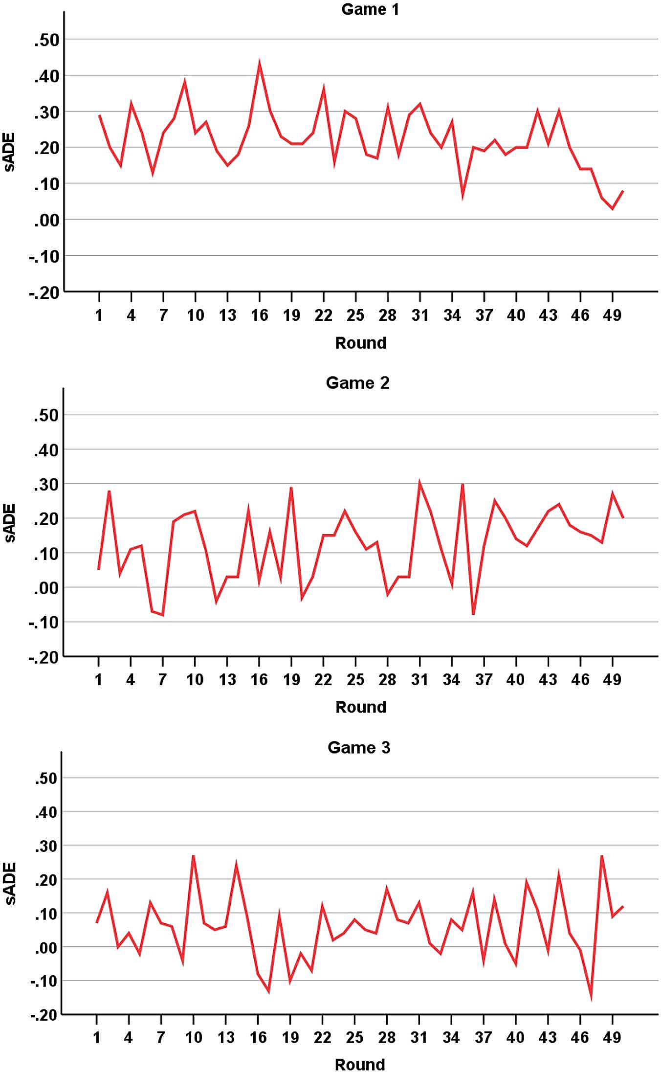
Fig. 2 Sequence plot of the sADE index across 50 rounds for Games 1, 2, and 3
The sequence plot for Game 2 also shows mainly positive values across the time series, confirming that the strategic asymmetric dominance effect established by the t test persisted over most of the 50 rounds of the repeated game, and there is no obvious trend, apart from rather high values in the last few rounds. The best-fitting model is ARIMA(0, 0, 0), indicating stationary noise, without any trend in the time series. Although a significant asymmetric dominance effect was found across the 50 rounds (using a conventional t test above), the time series analysis suggests that, in contrast to Game 1, there was no significant decline in the effect across the time series. For Game 2, stationary R 2 = 0.00, and Ljung–Box Q = 11.83, df = 18, p =.86, confirming that, although no significant variance is explained by the model, there is also no significant structure in the time series that is unexplained by the model.
For Game 3, the strategic asymmetric dominance effect fell short of statistical significance in a t test. The sequence plot for Game 3 shows mainly positive but also many negative values for sADE across the time series. The best-fitting model, as in Game 2, is ARIMA(0, 0, 0), indicating stationary noise without any trend. For this game, stationary R 2 = 0.00, and Ljung–Box Q = 22.23, df = 18, p =.22. This suggests that no significant portion of variance is explained by the model and no significant trend in the time series remains unexplained by the model.
Figure 3 shows the aggregate sequence plot of the sADE index across 150 rounds. This represents the time series for all 150 decisions made by the players in three different games played sequentially in different orders. Visual inspection suggests a very noisy time series with no obvious trend, or perhaps just the hint of piecemeal downward trends in rounds 1–50, 51–100, and 101–150. Time series analysis confirms the absence of any significant trend. The best-fitting model is a simple exponential smoothing model, in which each value is modeled as an exponentially weighted moving average of past values, without significant trend. This model is functionally equivalent to an ARIMA(0, 1, 1) model without a constant. The model fit statistics show stationary R 2 = 0.49, Ljung–Box Q = 29.87, df = 17, p =.027. The fact that the value of Q is narrowly significant for the 150-round time series confirms that some residual autocorrelation remains unaccounted for by the model, but there is no significant trend and hence no significant overall decline.

Fig. 3 Sequence plot of the sADE index for Games 1, 2, and 3 across 150 rounds
The significant Ljung–Box Q can be explained as follows. The time series in Fig. 3 incorporates the three 50-round time series in Fig. 2, but because our design controls for order effects, each of the three games is represented equally in rounds 1–50, 51–100, and 101–150 of the longer series. Bearing in mind that Game 1 showed a shallow but significant decline, this trend must be incorporated in each third of the 150-round sequence plot, because game order was systematically rotated, but the data from the other two games in each block of 50 rounds, together with the random variability in the data, tends to swamp the downward trend in each block. It is possible that this accounts for the unexplained autocorrelation in the time series indicated by the marginally significant Q value.
3.2 Verbal protocol analysis
The transcripts of verbal protocol sessions, from participants who did not take part in the main part of the study but were drawn from the same participant pool, were analyzed for themes relating to their understanding of the strategic properties of the games. Transcripts are available in the supplemental materials available on the OSF (https://osf.io/ph6ke). To play effectively, participants needed to try to anticipate what strategies their co-players would choose, and there were many instances in the verbal transcripts of the word hope/hoping and of searching for a pattern. Participants did try to understand what their co-players were doing and why they were doing it, and some of them clearly understood key aspects of the strategic structures of the games, but they were not adept at strategic thinking and did not always choose best responses even when correctly anticipating their co-players’ choices. This finding is consistent with those of a recent thorough quantitative investigation of (non-) best responding (Alempaki et al., Reference Alempaki, Colman, Kölle, Loomes and Pulford2022). Participants made many strategy choices without articulating clearly the reasons behind them, and this may perhaps suggest more impulsive than rational decision making.
Some participants clearly spotted the strategic asymmetric dominance in the games, although they did not always describe it articulately. For example, in Game 1, Participant 2 summed up the problem as follows: “E is like the non-safe option with like all the smaller numbers, and then D is like the non-safe option with like the big number and like small, and then C is like all the safe options, you know” (Round 44). Participant 3 repeatedly referred to C as the “safest bet” in Game 1, and Participant 2 repeatedly noted E (C in root position) as “the safe option” in Game 2. By round 20 of Game 1, Participant 5 resolved: “I’m gonna go for C constantly, ’cos it seems to have the higher values at C.” Participant 6 recognized the advantage of C and even concluded: “Yeah, I just wanna say C for the rest of the thing” (Round 38).
Some participants seemed to be making decisions as though the dominated E strategies could be ignored, and some seemed to treat the games like coordination games, or at least they made comments that are consistent with that interpretation. Participant 2 said in Game 1: “OK, what if I go for, I’m gonna go for D hoping for her to go for D as well, and the reason being I think there is chance I might end up getting money that way” (Round 9) and “OK, I’m gonna go for D hoping that she’ll go for D as well and we’ll get 80 80 each, OK” (Round 15) and “I’m gonna go for D hoping that she goes for D as well” (on Round 22). Player 3 commented in Game 1: “Gonna go for D again just in case they choose D as well” (Round 33). Player 5 commented in Game 1: “I’m gonna go for D hoping they choose D” (Round 26) and “OK, I’m gonna choose D assuming they’re picking D” (Round 46). In Game 2, Participant 6 (Red) said: “I’m gonna say C again ’cos I really want them to choose C” (Round 13), and on Round 32 she elaborated on this idea: “OK, I’m gonna choose C again ’cos we both chose C and it's a fair amount, 60 and 80.”
Many choices in the asymmetric games were clearly driven by inequity aversion: “I’m gonna go for D for the reason of getting equal numbers each” (Participant 3, Round 18), “I’m not gonna choose E just because I’m lower on that one and they get 80 and I get 60” (Participant 6, Round 10). However, Participant 5 preferred individual payoff maximization and said on Round 8: “I might stick to E the whole time ’cos I do have the higher numbers compared to [her].” Game 2 was perceived in a more competitive way by participants because of its payoff asymmetry, especially in the salient cells with the highest payoffs of 80. Participant 2 said in Round 14: “I think it's a bit more competitive this time” and by Round 26 was concerned that the co-player would get more money: “Next, I’m gonna go for E, I’m gonna go for my safe option I guess. . OK, so she got 80, I got 60, but that's the thing, we could both end up getting 60 60 or, um, she’ll end up getting more money than me.” This participant recognized the dominant strategy as a safer bet, but she did not stick with it reliably because of inequity aversion. Participant 8 demonstrated that her choices were driven by a competitive mindset: “I’m picking C again ’cos at least then we either don’t win anything or I win more than them” (Round 42). These comments suggest that the payoff inequity in cells with high payoffs in Game 2 functioned as a powerful distraction from the other strategic properties of the game, including especially the asymmetrically dominance relation between two of the strategies for both players.
None of the participants in this qualitative study commented on the possibility of alternation or rotation of strategies with their co-players. This might be expected in an experiment with fixed player pairs in repeated games with multiple Nash equilibria, especially games in which each player prefers a different equilibrium, such as repeated Battle of the Sexes or Chicken game. The participants in this qualitative study played 3 × 3 versions of Games 1 and 2. There would be no incentive to alternate in Game 1, because both equilibria offer the same payoffs to both players, whereas in Games 2, the players prefer different equilibria and such an incentive does exist. However, the availability of strictly dominant strategies for both players seems to have trumped any temptation to alternate.
4 Discussion and conclusions
Does the strategic asymmetric dominance effect persist or decay over repetitions in dyadic games? We shall argue that the effect decays, other things being equal, but the decay can be blocked in games that induce extraneous motives tending to counteract any decline in the effect. The results of our experiment show that the effect decayed significantly over 50 repetitions in Game 1 only, but the strategic structures of Games 2 and 3 induced in the players a powerful motive, extraneous to game theory, that may have prevented a similar decay over repetitions. Our findings may at first seem puzzling, but we believe that they are perfectly comprehensible in the light of this extraneous motivation. Before discussing the strategic properties of the three games that we believe provide a cogent explanation for our findings, we need first to address an apparent discrepancy between our results and those of Colman et al. (Reference Colman, Pulford and Bolger2007), from whose study we selected the three experimental games.
Our experimental games were the three investigated by Colman et al. (Reference Colman, Pulford and Bolger2007) that showed the largest asymmetric dominance effects in unrepeated (one-shot) decisions in that earlier study. Game 1 had shown the largest effect by far, and Games 2 and 3 the next largest effects, of the 18 games used in the earlier study. The most notable discrepancy between our findings and those of the earlier study relates to choices of dominated E strategies. In the earlier study, only between 0.69% (Experiment 1) and 2.47% (Experiment 2) of choices were of dominated E strategies, whereas in our current study, the corresponding percentages were 15.0% in Game 1, 30.0% in Games 2, and 23.3% in Game 3. There are two obvious explanations for this discrepancy. First, the earlier study investigated one-shot strategy choices, whereas the current study focused on repeated choices. It is unambiguously irrational to choose a dominated strategy in a one-shot game, but the folk theorem of repeated games (see Binmore, Reference Binmore1992, pp. 373–377, for a detailed mathematical exposition) shows, somewhat surprisingly, that this is not necessarily the case for repeated games. For example, in the one-shot Prisoner's Dilemma game, it is well known that choosing the dominated C strategy is irrational, and the only Nash equilibrium is joint defection, but in indefinitely repeated or iterated Prisoner's Dilemma, the folk theorem confirms that there are many Nash equilibria, including one in which both players choose C on every repetition. Therefore, on purely game-theoretic grounds, we should expect a smaller proportion of dominated strategy choices in one-shot games (as in the earlier study) than in repeated games (as in the current study).
Second, the participants in the earlier study were almost all undergraduate students studying economics, mathematics, or computer sciences, whereas those in the current study were undergraduate and graduate students from humanities, social science, and science departments, many of whom were probably comparatively unfamiliar with numerical and strategic reasoning, and that is another probable reason why they chose the dominated E strategy more frequently. Less numerically sophisticated participants should be expected to deviate more frequently from rational choice theory and game theory, but their inclusion in our current study sample has the considerable advantage, for an empirical investigation, of making the study more representative of the behavior of ordinary decision makers than the study of Colman et al. (Reference Colman, Pulford and Bolger2007). Given that the current study involved repeated games played by less numerically sophisticated decision makers, it would therefore have been surprising indeed if we had not observed a greater proportion of E choices than Colman et al.
Why was a significant decline in asymmetric dominance over repetitions observed only in Game 1? We believe that the probable explanation for this is inequity aversion or inequality aversion. It is well established that experimental participants tend to be strongly influenced by inequity aversion (Dawes et al., Reference Dawes, Fowler, Johnson, McElreath and Smirnov2007; Fehr & Schmidt, Reference Fehr, Schmidt, Kolm and Ythier2006; Han et al., Reference Han, Rapoport and Zhao2017; Rapoport et al., Reference Rapoport, Qi, Mak and Gisches2019), and we have observed it in many of our own previous experiments. In all three experimental games in the current study, the only Nash equilibria, in both the 2 × 2 control games and the 3 × 3 versions with asymmetrically dominated E strategies added, are the (C, C) and (D, D) cells, and these are also the only outcomes offering the highest possible payoff of 80 to one or both of the players. In all three games, the only dominance relation is the strict dominance by C of E in the 3 × 3 versions. In Game 1, because the game is symmetric, the (C, C) and (D, D) equilibrium outcomes are equally preferred by both players, either of these outcomes offering the maximum payoff of 80 to both players. If, as seems reasonable to assume, players’ understanding of the game increases over repetitions, then we should expect the strategic asymmetric dominance effect to decline over repetitions, which is what our data reveal. The asymmetrically dominated E strategy induced an initial preference for C over D that subsequently declined. It is likely to have become increasingly obvious to participants over repetitions that (C, C) and (D, D) are equally rewarding to both, and this probably explains why the initial preference for C over D—the asymmetric dominance effect—tended to decay.
In Games 2 and 3, on the other hand, a feature of the strategic structures appears to have prevented the effect from decaying. The (C, C) and (D, D) Nash equilibria are not equally preferred by both players: Player I prefers (C, C) and Player II prefers (D, D) in both games, but players are likely to be attracted toward these two equilibrium outcomes by the promise of potential maximum payoffs. Because inequity aversion is a powerful motive in experimental games, players are motivated to try to equalize the long-run frequencies of (C, C) and (D, D) outcomes as the most obvious way to achieve payoff fairness when the game is repeated. For the strategic asymmetric dominance effect to decline, the relative frequency of C choices relative to D choices has to decline, and this is prevented in Games 2 and 3 by any such pattern of choices motivated by inequity aversion.
It is worth commenting that our interpretation is in line with the finding of Amaldoss et al. (Reference Amaldoss, Bettman and Payne2008, Study 2), who reported persistence rather than decline of strategic asymmetric dominance in repeated Leader games with a weakly asymmetrically dominated strategy added for one player only. The Leader game has two Nash equilibria with unequal payoffs for the two players, as in our Games 2 and 3, and according to our interpretation, inequity aversion probably inhibited a decline of the strategic asymmetric dominance effect in that study. Our findings are also consistent with those of Ahn et al. (Reference Ahn, Kim and Ha2015), who reported that repetition weakens the asymmetric dominance effect in individual decision making, because in that study, as in our Game 1, there was no obvious factor inhibiting repetition-induced decline. Our findings and interpretation neither corroborate nor contradict those of Crosetto and Gaudeul (Reference Crosetto and Gaudeul2023), who reported evidence that the asymmetric dominance effect tends to decay almost immediately, as soon as players begin contemplating an individual decision. Unless the effect invariably disappears entirely before any decision is made—not something that Crosetto and Gaudeul claim to have shown—their finding says nothing about whether a residual effect, reflected in final decisions, persists or decays over subsequent repetitions.
The qualitative analysis reveals much evidence of inequity aversion and what seems at times like irrational blundering and guessing, flipping between choices with no apparent understanding of how to get high scores. This may have been due to the speed of decision making over multiple rounds in quick succession that may have tended to inhibit in-depth and rational strategic thinking. Asymmetric dominance effects have been shown to be larger when there is less time pressure and more time to detect the relationships and differences between options (Pettibone, Reference Pettibone2012). Some participants showed more strategic understanding than others but were flummoxed in their attempts at stable rational choices because they were paired with co-players who seemed to choose strategies arbitrarily or capriciously. Although some players showed inequity aversion, others were concerned with beating the other player, reflecting individual differences that influence strategy choice. These findings align with those of Pulford et al. (Reference Pulford, Krockow, Pinto and Colman2021) who also used verbal protocol analysis to study reasoning in dyadic matrix games and showed that people typically use multiple reasoning strategies when deciding, even in relatively simple games. However, we have shown that the verbal protocols also contain unmistakable evidence of strategic understanding and these help to explain the quantitative findings.
Drawing the threads of this unexpectedly complicated story together, the following conclusions seem reasonable. The asymmetric dominance effect, in both its individual and strategic forms, is clearly irrational. It is a type of context effect, resulting in a bias in judgment and decision making. Like the analogous context effect underlying the Müller-Lyer illusion in visual perception, the strategic asymmetric dominance effect tends to decline over repetitions, as players learn to understand the strategic properties of the game that they are playing and gravitate away from extraneous influences. However, there are factors outside the scope of orthodox game theory that can act as a brake on this decline. Among these are other-regarding preferences, in particular inequity aversion. In some games, inequity aversion can provide players with a motive to avoid decreasing the relative frequency of their asymmetrically dominant strategy choices over rounds, thereby inhibiting the decline in the effect that might otherwise occur, and there may be other extraneous factors that have a similar effect.
Acknowledgements
This work was supported by the Leicester Judgment and Decision Making Endowment fund [grant number M56TH33]. We are grateful to Holly Adams for transcribing the qualitative interviews, Marta Mangiarulo for helping with the literature search, and David Shanks for suggesting the investigation long ago.
Author contributions
Andrew M. Colman and Briony D. Pulford designed the study; all three authors drafted the manuscript; Alex Crombie collected the data and conducted the verbal protocol interviews; Briony D. Pulford and Andrew M. Colman analyzed the data and revised the manuscript.
Declarations
Competing interests
The authors declare no conflicts of interest with respect to the funding of this research and authorship of this article.


 Open access