


1 Introduction
Many models of investor behavior assume or imply that investors prefer assets with a positively skewed return distribution and dislike those with a negatively skewed return distribution (e.g., Arditti, Reference Arditti1967; Barberis & Huang, Reference Barberis and Huang2008; Brunnermeier et al., Reference Brunnermeier, Gollier and Parker2007; Dertwinkel-Kalt & Köster, Reference Dertwinkel-Kalt and Köster2019; Kraus and Litzenberger, Reference Kraus and Litzenberger1976; Scott & Horvath, Reference Scott and Horvath1980).Footnote 1 Such models can explain a wide range of important and puzzling patterns in investor behavior such as the tendency to underdiversify (e.g., Conine & Tamarkin, Reference Conine and Tamarkin1981; Simkowitz & Beedles, Reference Simkowitz and Beedles1978; Mitton & Vorkink, Reference Mitton and Vorkink2007), the surprising popularity of technical analysis (Ebert & Hilpert, Reference Ebert and Hilpert2019), or the pricing of skewness in the cross-section of stock returns (e.g., Boyer et al., Reference Boyer, Mitton and Vorkink2010). Given the potential explanatory power of a preference for skewness, it is critical to provide an empirical test of its relevance for investor behavior.
The key challenge for such a test lies in the fact that future returns to holding an asset are uncertain and investors have to form expectations about their distribution. Documenting the skewness of the expected return distribution at the level of the individual investor is therefore an important prerequisite for such a test.Footnote 2 However, despite a recently growing interest in measuring investors’ expectations and their relation to investment decisions (e.g., Drerup et al., Reference Drerup, Enke and von Gaudecker2017; Giglio et al., Reference Giglio, Maggiori, Stroebel and Utkus2021; Kuhnen & Miu, Reference Kuhnen and Miu2017), the skewness of investors’ return expectations has so far received no attention. In this paper, we fill this gap using high-quality data on individual return expectations and portfolio choices from a series of repeated, financially incentivized experiments with a representative sample of the Dutch population. We characterize the heterogeneity in expected skewness and relate it to portfolio choice at the individual level, both in the cross-section and over time.
Our data stems from a series of experiments which we ran with the Dutch LISS panel. In the experiments, we employed an intuitive graphical interface to obtain a fine-grained estimate for the distribution of each respondent’s return expectations for two risky assets, an index and a stock (Bellemare et al., Reference Bellemare, Bissonnette and Kröger2012; Delavande & Rohwedder, Reference Delavande and Rohwedder2008). We used these distributions to calculate estimates of the mean, standard deviation, and skewness of respondents’ expectations. In a complementary portfolio choice task, we asked respondents to allocate a fixed budget between the two risky assets and a savings account. To incentivize the belief elicitation procedure, we based respondents’ payouts at the end of the experiment on the accuracy of their beliefs. Likewise, we tied respondents’ payouts to the actual performance of their experimental portfolio at the end of the holding period, 1 year after the construction of the initial portfolio. Unannounced beforehand, we gave respondents the opportunity to update their beliefs and to change their portfolio allocations 6 months following the initial wave, adding a temporal dimension to the data.
This paper has two main contributions. First, we document individuals’ expectations concerning the distribution of returns, and in particular its skewness, for a broad index and an individual stock in a large, representative sample. Second, we show how these expectations relate to individuals’ portfolio choices.
Concerning the documentation of expectations, our selection of assets has several advantages. First, the chosen assets represent the main investment opportunities of a typical retail investor, i.e., well-diversified funds and individual stocks. Second, the fact that we elicit expectations for two assets also allows us to study the relation of beliefs across assets. In particular, we can explore whether expectations conform with common operationalizations of financial literacy stating that financially literate individuals should perceive investments into a mutual fund as safer than investments into a single company’s stock. The relation of expectations across assets might also help to shed light on the puzzling fact that many households invest significant fractions of wealth simultaneously in well-diversified mutual funds and in undiversified portfolios of individual stocks (e.g., Polkovnichenko, Reference Polkovnichenko2005). Skewness preferences have been used as one explanation for this observation but it has not been documented yet whether people actually perceive individual stocks as more skewed than funds.
We find that respondents entertain very heterogeneous skewness expectations, disagreeing not only on its magnitude, but also on its sign. While some respondents expect quite positively skewed return distributions for an asset, others expect negatively skewed distributions with small chances of drastic losses. Our respondents expect higher levels of skewness than what is observed in historical data for both the stock and index. In line with previous research (e.g., Ameriks et al., Reference Ameriks, Kézdi, Lee and Shapiro2019), respondents on average expect lower means and standard deviations of returns than historically observed. This underestimation is especially pronounced for the individual stock.
Employing the LISS panel’s rich background information, we next ask whether the heterogeneity in expected skewness can be traced back to socio-demographic characteristics. However, we find that these characteristics only explain very little of the variation. Stock market expectations seem to be intrapersonally stable but interpersonally highly variable (Dominitz & Manski, Reference Dominitz and Manski2011).
We conclude our documentation of expectations with an analysis of how the expectations for the two assets relate to each other. The data confirm the common intuition that individual stocks are perceived as more risky than a broad index of stocks. Dividing respondents into eight groups based on whether they expect a higher mean, standard deviation, and skewness, respectively, for the stock or the index, reveals that 40% of the subjects expect a higher mean, standard deviation, and skewness for the stock. Another 21% expect higher standard deviation and skewness for the stock, but a higher mean for the index.
To document the relation of stock market expectations and portfolio choice, we follow two approaches. First, we regress respondents’ initial investment in a given asset on the moments of respondents’ stated expectations for the asset. Respondents’ investments indeed increase with the skewness of the expected return distribution for each of the two assets. In other words, we find that respondents adjust their portfolio position in the stock in a way that is consistent with a preference for skewness.
In a second step, we exploit the repeated nature of the experiments. Using data from both the initial and the follow-up experiments 6 months later, we relate changes in the moments of the expectations for the asset at the individual level to changes in each asset’s holdings. For the asset with more temporal variation in skewness expectations, i.e., the stock, we find a positive relation between the changes in the expected skewness of the return distribution and changes in the respondents’ positions.
Our analysis contributes to several strands of literature. First, it complements a growing literature exploring the importance of skewness for investor behavior and asset prices. The study of skewness preferences in the stock market faces the problem that investors’ expected skewness is usually unknown. The existing empirical work uses an indirect approach to circumvent this problem by assuming that certain observable measures can serve as a proxy for expected skewness. Kumar (Reference Kumar2009) and Barberis et al. (Reference Barberis, Mukherjee and Wang2016), for example, assume that investors form beliefs by extrapolating the skewness of past returns into the future. Bali et al. (Reference Bali, Cakici and Whitelaw2011) and Lin and Liu (Reference Lin and Liu2017) proxy expected skewness by the maximum return of a stock over a certain period in the past. Others have, in the spirit of rational expectations, used future returns (e.g., Mitton & Vorkink, Reference Mitton and Vorkink2007) or options market data (Conrad et al., Reference Conrad, Dittmar and Ghysels2013).
These indirect approaches face two challenges. First, there is no consensus on what the best proxy for expected skewness is and over which time horizon it should be calculated. Second, models incorporating a preference for skewness are models about individual behavior. However, indirect approaches proxy expected skewness at the asset level and thus do not take heterogeneous expectations for a given asset across investors into account.Footnote 3
A number of papers in this literature document a negative correlation between the respective proxy for the expected skewness of an asset and subsequent returns. It is commonly suggested that a preference for skewness at the individual level is the mechanism driving this outcome, but this has been questioned (Barinov, Reference Barinov2018). One of our contributions is that we substantiate this mechanism by directly measuring expected skewness and showing that higher expected skewness at the individual level is linked to higher investment in an asset. More generally, our findings align with recent work (e.g., Das et al., Reference Das, Kuhnen and Nagel2019; Giglio et al., Reference Giglio, Maggiori, Stroebel and Utkus2021; Kuhnen and Miu, Reference Kuhnen and Miu2017) that suggests that taking heterogeneity in expectations into account is an important and fruitful direction for future research.
Second, our paper contributes to the literature studying higher order risk preferences in controlled experiments (see Trautmann & van de Kuilen, Reference Trautmann and van de Kuilen2018, for a review). A number of studies find that subjects (ceteris paribus) prefer more positively skewed lotteries in simple binary choice tasks (e.g., Deck & Schlesinger, Reference Deck and Schlesinger2010; Ebert, Reference Ebert2015; Ebert and Wiesen, Reference Ebert and Wiesen2011; Noussair et al., Reference Noussair, Trautmann and van de Kuilen2014). However, these studies are by design mute on the role of expectations since probabilities, payoffs, and hence the skewness of the return distribution are known in these experiments. Our contribution to this literature is that we extend the analysis to a situation in which returns are unknown.
Third, our findings also contribute to the literature on measuring stock market expectations. Due to the importance of stock market expectations as primitives of models of investor behavior, a substantial literature investigates how heterogeneous and accurate investors’ expectations are and how they relate to portfolio choices (e.g., Ameriks et al., Reference Ameriks, Kézdi, Lee and Shapiro2019; Amromin & Sharpe, Reference Amromin and Sharpe2014; Breunig et al., Reference Breunig, Huck, Schmidt and Weizsäcker2021; Das et al., Reference Das, Kuhnen and Nagel2019; Dominitz & Manski, Reference Dominitz and Manski2004; Drerup et al., Reference Drerup, Enke and von Gaudecker2017; Giglio et al., Reference Giglio, Maggiori, Stroebel and Utkus2021; Hudomiet et al., Reference Hudomiet, Kézdi and Willis2011; Hurd & Rohwedder, Reference Hurd and Rohwedder2012; Hurd et al., Reference Hurd, van Rooij and Winter2011; Kézdi & Willis, Reference Kézdi and Willis2011; Kuhnen & Miu, Reference Kuhnen and Miu2017; Vissing-Jorgensen, Reference Vissing-Jorgensen2003). However, possibly due to the prominence of the classical mean–variance framework (e.g., Markowitz, Reference Markowitz1952), the literature has characterized investors’ subjective expectations using at most the first two moments. Our main contribution to the expectations literature is that we extend the study of stock market expectations to include skewness. To our knowledge, we are also the first to elicit expectations for a broad index and an individual stock and are thus able to analyse the relation of expectations. In addition, we differ methodologically from most of the literature by paying participants for the accuracy of their beliefs. Many qualitative features of our incentivized expectations (e.g., underestimation of mean returns) replicate those previously found without incentives, thus alleviating concerns about the reliability of the latter.
Finally, unlike almost all previous work, we link expectations to investments in particular assets rather than stock market participation overall. In this aspect, our paper is closely related to Breunig et al. (Reference Breunig, Huck, Schmidt and Weizsäcker2021). In their portfolio choice experiment, subjects can invest in a stock whose return is drawn from the actual historical return distribution of the German DAX. They show that the mean of individual respondents’ estimates for this distribution predicts investment in the experimental stock. However, they do not study expected skewness.
2 Data
2.1 Data source
Our main source of data is the LISS panel of CentERdata at Tilburg University. The panel is a representative sample of the Dutch-speaking population permanently residing in the Netherlands. It is based on a true probability sample of households drawn from the population register. Overall, the panel consists of 4500 households comprising 7000 individuals who participate in monthly internet surveys. Our experiments were embedded in these surveys. In addition, a longitudinal survey is fielded in the panel every year, covering a large variety of domains like work, education, income, housing, time use, political views, values, and personality. Due to the high level of detail, in particular on households’ socioeconomic situation, data from the LISS panel and CentERdata have been used in a number of studies on investment behavior (e.g., Noussair et al., Reference Noussair, Trautmann and van de Kuilen2014; von Gaudecker, Reference von Gaudecker2015; van Rooij et al., Reference van Rooij, Lusardi and Alessie2011).
Our analyses employ data from a series of incentivized experiments. These experiments were conducted between August 2013 and November 2014. In our analyses, we restrict our attention to households who partook in August 2013, September 2013, and March 2014.Footnote 4 Within each household, the financial decision maker was asked to answer the questions. To ensure that all participants were at least minimally acquainted with financial decisions, households which did not report financial wealth in excess of €1000 were excluded. We include households whose financial wealth was unknown.
Figure 1 shows the temporal sequence of our experiments. In August 2013, participants were asked about their beliefs regarding the performance of two risky assets until August 2014. In September 2013, participants were asked for a point prediction for the interest rate of a standard savings account. In addition, they had to allocate €100 between the two assets and a savings account, knowing that they would be paid according to the performance of this portfolio in August 2014.Footnote 5 In March 2014, participants were again asked about their beliefs regarding the performance of the two risky assets until August 2014, and they were also given the opportunity to rebalance their portfolio. This second part of the experiments was not announced beforehand. Thus, when stating their initial beliefs and forming their portfolios, participants did not know that they would be allowed to adjust both at a later time. Importantly, this implies that belief elicitations and portfolio choice at both points in time were incentivized.Footnote 6
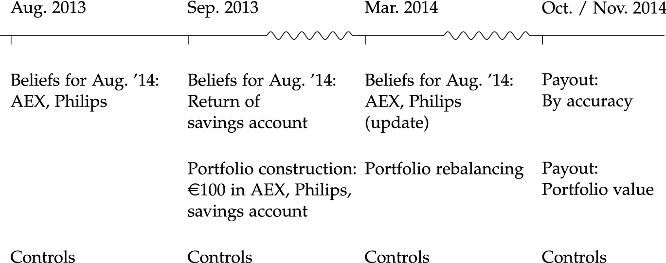
Fig. 1 Timeline
Table B.1 in the Internet Appendix provides an overview of response and attrition rates for the different points in time. Out of the 2978 individuals invited in August 2013, 77.6% completed the first experiment. In total, 1857 respondents completed all three experiments and comprise our main sample. The following sections describe the components of the experiments in more detail.
2.2 Experimental assets and time horizon
Throughout, the experiments contained two risky financial assets: shares of Koninklijke Philips N.V. (“Philips” in the following) and an exchange-traded fund invested into the Amsterdam Exchange Index (“AEX”). Both assets were likely recognized by all respondents in the sample. Philips is one of the biggest Dutch companies, and thus familiar to most if not all respondents in our sample. The same holds for the AEX, which is a broad and well-known index. As a benefit of employing real rather than artificial assets, the development of the assets’ actual prices provided a natural benchmark to incentivize respondents’ expectations. The experiments included detailed descriptions of each asset (see Sect. A.1 of the Appendix). In addition to shares of Philips and the AEX fund, the experiments also included a savings account. In the portfolio experiment, the savings account serves as an essentially riskless investment option.
When asking respondents for their expectations and portfolio decisions, the end of the holding period was held fixed. Thus, whenever respondents were asked for their expectations for a given asset, they were asked for the expected distribution of values in August 2014. Likewise, respondents were asked to construct portfolios with an investment-horizon ending in August 2014.
2.3 Eliciting expectations
To elicit respondents’ expectations, the experiments relied on a methodology proposed in Delavande and Rohwedder (Reference Delavande and Rohwedder2008). The method employs a graphical interface and lets respondents describe their expectations in the form of a histogram. Each respondent’s belief histogram in turn allows for a straightforward estimation of different moments of the respondent’s belief distribution. Sect. A.2 of the Appendix provides screenshots accompanying the following description of the design.
In August 2013, each respondent was asked to imagine an investment of €100 each into either Philips or the AEX. The respondent was then asked to think about the value of each of these investments in August 2014 (i.e., in 1 year).Footnote 7 Next, respondents were asked to express their expectations using a graphical interface (see Fig. 3).
Using the interface, respondents could distribute a total of 100 balls across 8 distinct bins to express their confidence that the value of each asset would fall into certain intervals represented by each bin. The allocation of balls proceeded iteratively. Initially, the respondents were asked to distribute all 100 balls to two intervals,
 and
and
 , to indicate their confidence that the value of their investment would fall below or above €100. Next, the interface asked respondents to redistribute all balls they had assigned to
 into two sub-intervals, (100, 105] and
 . This continued until respondents had allocated all balls to eight intervals. While the six interior intervals covered €5 ranges of possible values each, the two outer bins represented open intervals,
 and
and
 .
.
Unannounced beforehand, respondents were given the chance to adjust their expectations using a slightly adapted version of the interface in March 2014 (see Fig. 4). Participants were informed about the performance of the respective asset since the last elicitation of beliefs before being given the opportunity to revise their beliefs. On average, the performance of the AEX was 5% (Philips 1.7%) between the first and second elicitation of beliefs. The new interface initially presented them with the distribution of expectations they had stated in August 2013. Below each bin, the interface now contained +/− signs that allowed respondents to adjust the probability that the final value of the asset would fall into the respective bin.
To account for variation in respondents’ expectations for the savings account, respondents were also asked to provide a point estimate for its rate of return. Section A.4 of the Appendix provides a detailed description of this part of the experiment and the distribution of point estimates in our sample.
An alternative way of eliciting expectations would have been to use a probabilistic question format (Manski, Reference Manski2004). This approach relies on a series of questions of the form: “What do you think is the percent chance that the return on asset X will be larger than value Y?” The two approaches are equivalent in the sense that both can be used to estimate the third moment of respondents’ expectations. In our view, however, the design proposed by Delavande and Rohwedder (Reference Delavande and Rohwedder2008) has two very important practical advantages. First, the answers to Manski-type probabilistic questions are often internally inconsistent (Binswanger & Salm, Reference Binswanger and Salm2017). That is, many subjects violate monotonicity. Most studies exclude these subjects, leading to a substantial reduction in sample size and unwanted selection effects. Our design enables us to make use of the full sample. In addition, monotonicity violations are likely to become more severe or frequent as the number of questions asked increases. It would take seven questions to obtain the same resolution as our approach. Second, the design by Delavande and Rohwedder (Reference Delavande and Rohwedder2008) is intuitive and easy to understand which is especially important in a representative sample such as ours. The approach has been used successfully with samples of poor, illiterate subjects in developing countries (see Delavande et al., Reference Delavande, Giné and McKenzie2011, for a review).
2.4 Estimating the moments of respondents’ expectations
To obtain estimates for the entire distribution of a respondent’s expectations and its moments, we followed a variant of the methodology suggested in Bellemare et al. (Reference Bellemare, Bissonnette and Kröger2012). First, we turned the histograms into discrete cumulative distribution functions of a respondent’s expectations. For example, when a respondent put 5 balls into the bin
 and 5 more into (85, 90], we set the value of the CDF at 85 and 90 to 0.05 and 0.10, respectively. Second, we connected each pair of neighboring points on this CDF through a monotonically increasing cubic polynomial (i.e., a cubic Hermite spline) to obtain an estimate of the CDF between two bin boundaries. Afterwards, we combined the resulting 8 polynomials into one continuous function to serve as our estimate for the entire distribution of beliefs. Basically, this method takes the discrete distribution of expectations and turns it into a smooth estimate of the continuous distribution by connecting all known points through suitably chosen polynomials.
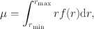
After expressing this estimate in returns (i.e., after shifting the support by −100), we calculated the mean, standard deviation, and skewness of the expected return distributions. Specifically, for each respondent, each point in time at which expectations were elicited, and each asset, we calculated the expected mean
 as
as
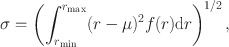
the expected standard deviation
 as
as
and the expected skewness
 as
as
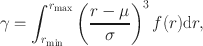
by integrating over the entire support of our estimate for the distribution of expected returns
 . We set the limits of integration (
 and
and
 ), i.e., the outer bounds of the extreme bins, to the 5th and 95th percentile of the distribution of the respective asset’s historical returns. We obtain qualitatively similar results when we pick more extreme outer bounds.
In Sect. B.3.1 of the Internet Appendix, we provide a more detailed description of the method, including its technical implementation. We also show some estimated distributions and their moments.
The expectations elicited in August 2013 and March 2014 both concern the same time period (August 2013 until August 2014) and are, therefore, directly comparable. However, for the portfolio choice decision in March 2014, expectations about the performance of the assets between March 2014 and August 2014 matter. These can be backed out from the stated expectations by taking the performance of the assets until the second elicitation of expectations in March 2014 (about which participants were informed before making their decision) into account. In the regressions explaining changes in portfolio choices reported below we use these backed out expectations to calculate the difference in expected moments (more details on the calculation are provided in Internet Appendix B.6.1.3).
The choice of method is the result of several trade-offs. Evidently, time constraints prevented asking respondents to distribute, say, 10,000 balls across 100 bins to obtain an even more fine-grained estimate for the discrete distribution of expected returns. The interpolation of the distribution between a reduced set of known points seems a natural alternative. At the same time, there are, of course, several ways to interpolate this distribution. An alternative to our approach would have been to impose a parametric shape for the entire distribution and to obtain estimates of its moments based on the assumed functional form. Our approach is a little more flexible in that it can handle varying distributional shapes between bins, thus allowing for less “well-behaved” beliefs. Also, we felt more comfortable not imposing a parametric distribution to avoid potential problems arising from misspecification.
2.5 Portfolio choice experiment
The first round of the portfolio choice experiment was fielded in September 2013. In the experiment, the same set of respondents that was initially surveyed for their expectations was asked to invest a total amount of €100 into nonnegative positions of the AEX index fund, shares of Philips, and a savings account for a 1-year investment horizon. Respondents were told that the value of each asset position would be tied to the actual return of the asset. A decline in the value of the AEX between September 2013 and August 2014, for example, would have reduced the value of the AEX share in a portfolio at the end of the experiment. To facilitate portfolio construction, an intuitive graphical interface was shown to respondents (see Fig. 8 in the Appendix). The interface allowed respondents to select and adjust individual portfolio positions by moving sliders up and down. They could only proceed with the survey once they had allocated an amount of exactly €100.
Unannounced beforehand, respondents were allowed to adjust their portfolio compositions in March 2014. First, they were presented with the portfolio they had initially chosen, adjusted for intermediate returns between September 2013 and March 2014. Respondents could then adjust the portfolio’s positions. Again, respondents were required to allocate the full value of the portfolio, which now varied between respondents, before they were allowed to proceed with the survey.
2.6 Additional variables
Our analyses employ a number of control variables. From the LISS background panel, we obtain information on respondents’ gender, marital status, children, age, financial wealth, income, and education (for definitions and summary statistics, see Appendix A.6). The “Preference Survey Module” of Falk et al. (Reference Falk, Becker, Dohmen, Huffman and Sunde2016) was employed to obtain measures for a respondent’s level of risk aversion (see Appendix A.7 for detailed results).
2.7 Incentives
Recent findings (e.g., Palfrey & Wang, Reference Palfrey and Wang2009) suggest that financial incentives can lead to more truthful reporting of beliefs. The elicitation of beliefs was incentivized using the binarized scoring rule of Hossain and Okui (Reference Hossain and Okui2013). This scoring rule addresses the concern that risk averse individuals have an incentive to report less dispersed beliefs under the often used quadratic scoring rule. Under the binarized scoring rule, the quadratic score does not directly translate into a payoff and instead generates a chance of winning a high rather than a low fixed prize. To this end, we first randomly drew one of the two assets for each respondent. We then calculated the following sum for the chosen asset:
 was the number of balls in bin
 and
and
 equalled 1 if the realized value of a €100 investment fell into the respective bin (and 0 otherwise). The sum thus reflected how far the elicited belief distribution was from the actual value. Next, we checked whether the sum of squared deviations fell above or below a randomly drawn number from a uniform distribution (U[1, 20.000]). If it was larger, a participant would receive €100 conditional on being selected for payment.Footnote 8
As is common practice with large samples like ours, we randomly selected one in ten participants for payment in October 2014. To ensure that participants had incentives to thruthfully report their expectations in August 2013, we did not tell them that they would be able to adjust their expectations in March 2014.
In the portfolio construction task, 1 in 10 respondents was independently drawn to receive the value of the portfolio at the end of the experiment. Again, we did initially not tell participants that they would be able to adjust their portfolios. The random draws for the belief elicitation task and the portfolio choice task were independent.
Incentives were based on expectations and portfolio decisions from March 2014. This ensured that respondents had incentives to update both. In the belief elicitation task, the average respondent earned €39.66 conditional on being selected for payment (unconditional earnings €3.98). The average portfolio value of respondents being selected for payment in the portfolio task was €104.42 (unconditional earnings €9.62).
3 Expected skewness: heterogeneity and determinants
This section begins with descriptive statistics of return expectations, focusing on the distribution of the skewness of respondents’ expected return distributions. We then turn to possible determinants of variation in skewness expectations before we analyze the relation of expectations across assets.
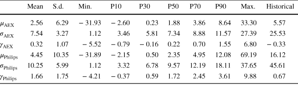
Figure 2 presents the cross-sectional distributions of the skewness parameters of respondents’ return expectations for the AEX and Philips.Footnote 9 Table 1 shows several characteristics of these distributions alongside information on the first and second moments. The dashed lines in the figures present the skewness of the assets’ historical return distributions, also shown in the last column of the table (for their calculation, see Sect. B.4 of the Internet Appendix).
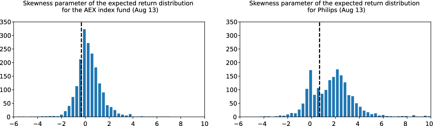
Fig. 2 Distribution of the skewness parameters of the expected return distributions. Distribution of the skewness parameters of the expected return distributions for an investment in the AEX index fund (left) and Philips (right) between August 2013 and August 2014. Figure B.4 of the Internet Appendix contains the distribution of skewness expectations in March 2014
Sources: LISS panel/yahoo! finance/Statistics Netherlands/own calculations
Table 1 Distribution of the estimated moments of the expected return distributions
|
Mean |
S.d. |
Min. |
P10 |
P30 |
P50 |
P70 |
P90 |
Max. |
Historical |
|
|---|---|---|---|---|---|---|---|---|---|---|
|
|
2.56 |
6.29 |
− 31.93 |
− 2.60 |
0.23 |
1.88 |
3.86 |
8.64 |
33.30 |
5.57 |
|
|
7.54 |
3.27 |
1.12 |
3.46 |
5.81 |
7.34 |
8.88 |
11.57 |
27.39 |
25.53 |
|
|
0.32 |
1.07 |
− 5.52 |
− 0.79 |
− 0.16 |
0.22 |
0.70 |
1.55 |
6.80 |
− 0.33 |
|
|
4.45 |
10.35 |
− 31.89 |
− 2.15 |
0.50 |
2.35 |
4.95 |
12.08 |
69.19 |
16.12 |
|
|
10.25 |
5.99 |
1.12 |
3.32 |
6.78 |
9.57 |
12.19 |
18.11 |
37.65 |
45.61 |
|
|
1.66 |
1.75 |
− 4.21 |
− 0.37 |
0.59 |
1.72 |
2.45 |
3.61 |
9.88 |
0.67 |


The table shows characteristics for the distribution of the moments of respondents’ expectations for the 1-year returns of the AEX (top three rows) and Philips (bottom three rows) in August 2013. The last column shows the respective historical moment, i.e., the moment of the empirical distribution of 1-year returns (see Sect. B.4 in the Internet Appendix)
Sources: LISS panel/yahoo! finance/Statistics Netherlands/own calculations
One aspect stands out in particular. There is a lot of heterogeneity in respondents’ skewness expectations. For the AEX, the average skewness of respondents’ return expectations is 0.32 with a standard deviation of 1.07. For Philips, the average skewness is 1.66 with a standard deviation of 1.75. Thus, for both assets there is substantial variation in the skewness of respondents’ return expectations, though the skewness of expectations for Philips seems more variable across respondents. Interestingly, respondents do not only disagree on the size of the expected skewness, but also on its sign. For example, about 62% expect a positively skewed return distribution for the AEX, whereas 38% expect the opposite. Put differently, there are some respondents who expect the AEX to offer small chances of large gains, while others expect small chances of large losses. For Philips, with 83% of respondents expecting a positively skewed return distribution, there seems to be less disagreement on the sign of the skew.
Relative to the skewness of the historical distributions of both assets’ returns, our respondents’ expectations tend to be comparably high. For example, while the historical distribution of AEX returns had a skewness of
 , respondents in the sample on average expect a return distribution with a skewness of 0.32. Taken together, respondents’ skewness expectations are highly heterogeneous. Our results also suggest that historical values of skewness provide only poor proxies for the skewness of most respondents’ return expectations.
The statistics on the first two moments of respondents’ expectations, shown in Table 1, can be used for a quality check of our data. In line with recent work in which the elicitation of beliefs was not incentivized, we find that respondents’ expected returns (Giglio et al., Reference Giglio, Maggiori, Stroebel and Utkus2021; but see Breunig et al., Reference Breunig, Huck, Schmidt and Weizsäcker2021) and standard deviations (Ameriks et al., Reference Ameriks, Kézdi, Lee and Shapiro2019) are very heterogenous and they tend to be lower than the historical averages.Footnote 10
We next turn to the analysis of what drives skewness expectations. In the analysis, we focus on characteristics which have also been considered as determinants of subjective stock market expectations in prior work (e.g., Das et al., Reference Das, Kuhnen and Nagel2019; Hudomiet et al., Reference Hudomiet, Kézdi and Willis2011; Hurd et al., Reference Hurd, van Rooij and Winter2011; Kuhnen & Miu, Reference Kuhnen and Miu2017: gender, age, education, income, financial wealth, marital status, and having children. Finding systematic differences in skewness expectations would, in combination with a preference for skewness, provide a potential explanation why sociodemographic groups differ in their tendencies to hold positively skewed stocks as it has been documented, for example, in Kumar (Reference Kumar2009).
Table B.5 in the Internet Appendix shows regressions of respondents’ expected skewness for each asset on these potential determinants. The regressions do a poor job at explaining variation in expected skewness. The
 s are very low and, with the exception of one age dummy in each and the dummy for having children in the AEX regression, none of the covariates shows up significantly.
Several aspects of the data suggest that this is not due to the specifics of the method we employ to measure respondents’ expectations or due to noise in the data. First, Sect. B.3.4 in the Internet Appendix shows that the observed patterns in the mean and standard deviation of respondents’ expectations conform to results from prior work in many regards (e.g., Dominitz & Manski, Reference Dominitz and Manski2004; Hurd, Reference Hurd2009; Hurd et al., Reference Hurd, van Rooij and Winter2011). For example, we find that male respondents and those who report more financial wealth tend to have a higher mean estimate for the AEX. In line with Giglio et al. (Reference Giglio, Maggiori, Stroebel and Utkus2021), we also find that
 tends to be quite low in these regressions.
Second, respondents seem fairly consistent in their expectations across assets. In September 2013, the pairwise correlations between the mean, standard deviation, and skewness of respondents’ expectations for the AEX and Philips were 0.41, 0.47, and 0.14, respectively (see Sect. B.3.4 in the Internet Appendix). Put differently, respondents whose expectations tend to have higher means, standard deviations, or skewness for one asset also tend to have higher values for the other. We consider it unlikely that the method should pick up this consistency but at the same time perturb the measured expectations enough to obscure underlying determinants. The low explanatory power of our observables also aligns with the result of Giglio et al. (Reference Giglio, Maggiori, Stroebel and Utkus2021) that individual fixed effects drive most of the temporal variation in beliefs about mean stock market returns. Third, data on respondents’ expectations from this experiment has been shown to predict behavior in the field (Drerup et al., Reference Drerup, Enke and von Gaudecker2017), and, as we will see in the next section, variation in expectations also predicts variation in experimental behavior.
We next analyze how the expectations for the two assets relate to each other. 57% of participants expected a higher mean for Philips, 71% expected a higher variance, and 77% expected a higher skewness. Overall, the data thus confirm the common intuition that individual stocks are perceived as riskier than a broad index of stocks. The data also provide evidence for skewness-based explanations of the fact that many households simultaneously invest in well-diversified mutual funds and in undiversified portfolios of individual stocks (Polkovnichenko, Reference Polkovnichenko2005) in the sense that our participants expect a higher skewness for the individual stock than for the broad index. We divide participants into eight different groups based on whether they expect a higher mean, standard deviation, and skewness, respectively, for Philips or for AEX. Altogether, 40% of the subjects expect a higher mean, standard deviation, and skewness for Philips and 21% expect higher standard deviation, and skewness for Philips but a higher mean for the AEX. The shares of the other six groups are much smaller (as reported in Table B.2 in the Internet Appendix).
As our final analysis of heterogeneity in and determinants of beliefs, we take a closer look at whether and how participants changed their beliefs at the second elicitation in March 2014. Table B.3 of the Internet Appendix provides information about the distribution of changes in participants’ beliefs for the AEX and Philips. While the expected return for the AEX increases and the one for Philips decreases, participants slightly reduce their expected variance and skewness for both assets. This could reflect the fact that the period between the two belief elicitations was a period of relative stability in the stock market during which the AEX outperformed Philips. In terms of portfolio shares, the share invested in the AEX goes up by 3 percentage points (8.6%), the share invested in Philips goes down by 0.6 percentage points (2%), and the share held in the savings account decreases by 2.4 percentage points (7.6%). In Table B.4 of the Internet Appendix we provide an overview of the share of participants that increase, decrease, or do not change their beliefs about mean, standard deviation, and skewness of the two assets. The table shows that only slightly more than 50% of participants adjusted their beliefs.
4 Heterogeneity in expected skewness and portfolio choice
When constructing their portfolios in September 2013, respondents favored the AEX over investments in Philips or the savings account, with average fractions of 35%, 33%, and 32%, respectively.Footnote 11 This tendency became more pronounced in March 2014 with the average portfolio shares changing to 38% in the AEX, 32% in Philips, and 30% in the savings account. There was substantial heterogeneity in both how respondents composed their portfolios and in how they adjusted them over time. The standard deviation of the share invested into Philips in September 2013, for example, was 24%.
In this section, we relate respondents’ stated expectations to their behavior in the portfolio choice experiment. Before we present the results, we discuss our choice of regression setup. Most of the literature on the role of stock market expectations rests on the mean-variance paradigm of classical portfolio choice theory (Markowitz, Reference Markowitz1952; Merton, Reference Merton1969). Accordingly, the focus often lies on regressions relating expected mean (and variance) for a broad index of stocks to stock market participation or the share of financial wealth invested in stocks. One appealing feature of the Merton model is that the first order condition can be transformed into an additively separable function of the expected mean and variance. The model thus suggests a specific regression specification with clear quantitative predictions about the size of coefficients. Once we move away from the first and second moment of returns and add skewness to the model, this is no longer the case. The first order conditions become more complicated and cannot be transformed into an additive separable function of mean, variance, and skewness, even for the case of a single asset.
In addition, a number of models like Brunnermeier et al. (Reference Brunnermeier, Gollier and Parker2007), Mitton and Vorkink (Reference Mitton and Vorkink2007), or Barberis and Huang (Reference Barberis and Huang2008) use very different approaches to motivate skewness preferences.Footnote 12 Absent an easily tractable or commonly agreed upon framework, we focus on documenting the qualitative relation between stock market expectations and portfolio choice. We, therefore, use linear regressions of portfolio allocation decisions on expected moments of the return distribution.
Another difference to the previous stock market expectations literature is worth pointing out. What matters to the investor in most models are the expected overall moments of the portfolio returns which depend on the expected returns of the individual assets in the portfolio and their co-moments. The standard approach in the literature on the mean-variance framework is to directly ask about proxies of overall expected return and variance of an individual’s portfolio (e.g., expectations for an index, or stocks in general). In contrast, as motivated above, we deliberately elicit expectations for two specific assets. However, we do not elicit their joint distribution. We are only aware of one attempt to elicit the joint distribution for two assets (Drerup, Reference Drerup2019), and the complexity of the task and the time required ruled out its use in our experiment.Footnote 13 We can thus not calculate the overall expected portfolio moments.
Our regression results can nevertheless inform the literature on skewness preferences in important ways. First, the only paper which explicitly models portfolio choice with two skewed assets (Beddock & Karehnke, Reference Beddock and Karehnke2021) suggests that higher expected skewness of an asset’s returns will ceteris paribus increase the portfolio weight of that asset assuming exponential utility (or CPT) and a split bivariate normal return distribution. This prediction is independent of the correlation between the assets and can be tested with our analysis.
Second, some models (Barberis & Huang, Reference Barberis and Huang2008; Brunnermeier et al., Reference Brunnermeier, Gollier and Parker2007) also suggest that the skewness of individual securities in itself may directly influence investors’ portfolio decisions.Footnote 14 A substantial number of papers provide indirect evidence for this by documenting a negative correlation between proxies for the expected skewness of an asset and subsequent returns (e.g., Boyer et al., Reference Boyer, Mitton and Vorkink2010; Conrad et al., Reference Conrad, Dittmar and Ghysels2013; Mitton & Vorkink, Reference Mitton and Vorkink2007). Our analysis goes one step further by directly measuring expected skewness for individual assets and testing whether higher expected skewness at the individual level is linked to higher investment in an asset.
Third, under the additional assumption that respondents perceive the assets to be positively correlated, our regression can test the prediction of Beddock and Karehnke (Reference Beddock and Karehnke2021) that an increase in one asset’s skewness decreases the amount invested into the other asset. Support for this assumption comes from the only paper which we are aware of to explicitly look into perceived correlation (Drerup, Reference Drerup2019). The setup is similar to ours in the sense that he elicits the joint distribution for an index (the German DAX) and two stocks from that index. For both of these stocks the majority of subjects expects positive correlations with the DAX.Footnote 15 Finally, we hope that the regressions reported below can help guide the development of future models that explore the relationship between beliefs, portfolios, and ultimately asset prices.
Using our basic regression setup, we approach the question of how skewed return expectations relate to investment decisions in two different ways: First, we explore the contemporary association between a participant’s expectations concerning the skewness of an asset’s return distribution and the share invested into the same asset in the portfolio choice experiment. Second, we exploit the repeated nature of our experiments and link variation in a respondent’s expected skewness between August 2013 and March 2014 to variation in investment shares between September 2013 and March 2014. Thus, we assess the potential relevance of preferences for skewness both through the relation between expectations and investments at a given point in time as well as through the relation between changes in expectations and changes in investment decisions over time.
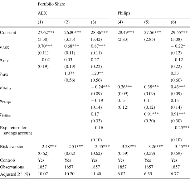
We begin the presentation of results in Table 2. The table shows regression of portfolio shares for the AEX (columns 1–3) and Philips (columns 4–6) on different moments of the expected distribution of returns and a measure of risk aversion (described in Sect. A.7). Based on the previous literature on stock market expectations (e.g., Das et al., Reference Das, Kuhnen and Nagel2019; Hurd et al., Reference Hurd, van Rooij and Winter2011; Hudomiet et al., Reference Hudomiet, Kézdi and Willis2011; Kuhnen & Miu, Reference Kuhnen and Miu2017), all specifications include controls for gender, age, education, marital status, children, income, and financial wealth. To maintain brevity, we only report the coefficients of these controls in Table B.8 of the Internet Appendix and focus on the expectation variables here. In the first column of Table 2, we show the results of regressing the share invested into the AEX only on the first two moments of expectations for the AEX. In the second column, we add the skewness of the expected return distribution for the AEX. In the third column, we add the point estimate for the return of the savings account and the moments of Philips’ expected return distribution to control for the subjective attractiveness of alternative assets.
Table 2 Expectations and portfolio choice.
Sources: LISS panel and own calculations
|
Portfolio Share |
||||||
|---|---|---|---|---|---|---|
|
AEX |
Philips |
|||||
|
(1) |
(2) |
(3) |
(4) |
(5) |
(6) |
|
|
Constant |
27.62*** |
26.80*** |
28.86*** |
28.49*** |
27.56*** |
29.55*** |
|
(3.30) |
(3.33) |
(3.42) |
(2.83) |
(2.85) |
(3.08) |
|
|
|
0.70*** |
0.68*** |
0.87*** |
− 0.22* |
||
|
(0.11) |
(0.11) |
(0.11) |
(0.12) |
|||
|
|
− 0.02 |
0.03 |
0.27 |
− 0.12 |
||
|
(0.19) |
(0.19) |
(0.22) |
(0.22) |
|||
|
|
1.07* |
1.20** |
0.33 |
|||
|
(0.56) |
(0.56) |
(0.60) |
||||
|
|
− 0.24*** |
0.36*** |
0.38*** |
0.43*** |
||
|
(0.09) |
(0.09) |
(0.09) |
(0.09) |
|||
|
|
− 0.19 |
0.15 |
0.11 |
0.15 |
||
|
(0.14) |
(0.12) |
(0.12) |
(0.14) |
|||
|
|
0.17 |
0.91*** |
0.91*** |
|||
|
(0.33) |
(0.30) |
(0.30) |
||||
|
Exp. return for savings account |
− 0.16 |
− 0.25*** |
||||
|
(0.10) |
(0.10) |
|||||
|
Risk aversion |
− 2.48*** |
− 2.51*** |
− 2.45*** |
− 3.28*** |
− 3.26*** |
− 3.45*** |
|
(0.62) |
(0.62) |
(0.62) |
(0.59) |
(0.59) |
(0.59) |
|
|
Controls |
Yes |
Yes |
Yes |
Yes |
Yes |
Yes |
|
Observations |
1857 |
1857 |
1857 |
1857 |
1857 |
1857 |
|
Adjusted R
|
10.07 |
10.20 |
11.40 |
6.02 |
6.39 |
6.77 |


The table contains OLS regressions of the share invested into the AEX (columns 1–3) and Philips (columns 4–6) on varying sets of covariates. In addition to the variables shown in the table, the regressions include controls for gender, age, education, marital status, children, income, and financial wealth. The missing coefficients are shown in Sect. B.5 of the Appendix. Section A.6 defines all controls that have not been defined in the main text. Heteroskedasticity-robust standard errors are reported in parentheses
The coefficient of the mean expected return,
 , is positive and highly significant in columns 1, 2, and 3. Respondents’ shares invested into the AEX thus increase with their mean return expectation, suggesting a positive preference for higher mean returns. The effect is economically substantial. An increase in the expected mean return for the AEX by one standard deviation increases the AEX’s fraction in the experimental portfolio by approximately 5.41 percentage points or about 15.46% of the unconditional average of the share invested into the AEX.Footnote 16 Put differently, an increase in the expected mean return by one percentage point increases the share invested into the AEX index fund by 0.7 percentage points. The size of this coefficient is remarkably close to the estimates of Giglio et al. (Reference Giglio, Maggiori, Stroebel and Utkus2021). The standard deviation of the expected distribution,
 , does not enter significantly in any of the specifications. Thus, how much the average respondent invests into the AEX seems unaffected by the expected riskiness of the AEX’s future returns in terms of their expected standard deviation. This finding is also in line with the findings of Breunig et al. (Reference Breunig, Huck, Schmidt and Weizsäcker2021) and Giglio et al. (Reference Giglio, Maggiori, Stroebel and Utkus2021).
The coefficient of the expected skewness,
 , is positive and significant with
 -values below 0.10 and 0.05 in both column 2 and 3. Respondents expecting a more positively skewed return distribution thus invest larger shares of their portfolios into the AEX, suggesting a preference for higher skewness. The effect is again economically meaningful. As expected, the coefficient for the mean return expectation for Philips in column 3 is negative and significant.
Columns 4–6 show analogous regression results for respondents’ investments in Philips. The results provide strong confirmation of the findings for the AEX. The coefficient of the mean expected return for Philips,
 , is positive and highly significant in all three specifications. The standard deviation,
 , again enters nonsignificantly. The coefficient of the expected skewness,
 , is positive and significant with
 -values of less than 0.01 in both column 5 and 6. The results for investments in Philips are thus also consistent with a positive preference for both higher mean returns and more skewed return distributions, whereas they do not suggest any preference concerning standard deviations. The economic magnitudes of the effects are remarkably similar to those of the effects associated with the AEX.Footnote 17
Two other findings are worth pointing out. First, risk aversion is associated with reduced investment in both risky assets. Second, note that investment into an asset is negatively correlated with the expected mean for the other asset but not with the other asset’s skewness. The latter is not in line with Beddock and Karehnke (Reference Beddock and Karehnke2021) if we assume that respondents expect a positive correlation between Philipps and the AEX. In their model, demands for the two skewed assets are only independent of each other in the case of no correlation.
Another interesting question is whether the correlation between investments and expected skewness is driven by a particular dislike for negative skewness similar to the idea of rare disasters in the macro-finance literature, or a particular preference for positive skewness (e.g., ”lottery stocks”). In Table B.23 of the Internet Appendix we replicate the static main regression and include separate terms for positive and negative skewness. In both static regressions, all coefficients are as expected; positive skewness is associated with an increase in the portfolio share of an asset, whereas negative skewness is associated with a reduction. With the exception of positive skewness for the AEX, all coefficients are significant at the 10% level or less. The coefficients for positive and negative skewness are not significantly different from each other (Wald tests reported in Sect. B.6.5). The results thus do not provide strong evidence concerning differential effects of positive and negative skewness.
In sum, cross-sectional variation in expectations and portfolio choices at a fixed point in time is in line with a preference for assets with higher mean returns as well as more positively skewed return distributions. Variation in the standard deviation of respondents’ expectations does not seem to be associated with variation in their portfolio shares.
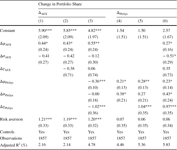
For our dynamic analysis, we rely on the same regression format as before, but we replace the static portfolio decisions and expectations with the respective changes. Thus, we regress changes in portfolio shares between September 2013 and March 2014 on changes in the moments of respondents’ expected return distributions between August 2013 and March 2014 (see Sects. 2.4 and B.6.1.3 for the calculation of the latter). We run the regressions both with and without the changes in the respective other asset’s expected return distribution and we include the sociodemographic control variables. Table 3 shows the results.
Table 3 Changes in expectations and portfolio dynamics.
Sources: LISS panel and own calculations
|
Change in Portfolio Share |
||||||
|---|---|---|---|---|---|---|
|
|
|
|||||
|
(1) |
(2) |
(3) |
(4) |
(5) |
(6) |
|
|
Constant |
5.90*** |
5.85*** |
4.82*** |
1.54 |
1.50 |
2.57 |
|
(2.09) |
(2.09) |
(1.97) |
(1.51) |
(1.51) |
(1.67) |
|
|
|
0.44* |
0.43* |
0.55** |
0.27* |
||
|
(0.24) |
(0.24) |
(0.24) |
(0.16) |
|||
|
|
− 0.41 |
− 0.42 |
− 0.12 |
− 0.51* |
||
|
(0.27) |
(0.27) |
(0.30) |
(0.29) |
|||
|
|
− 0.38 |
0.06 |
0.35 |
|||
|
(0.71) |
(0.74) |
(0.73) |
||||
|
|
− 0.36*** |
0.21* |
0.28** |
0.23* |
||
|
(0.10) |
(0.13) |
(0.13) |
(0.14) |
|||
|
|
− 0.00 |
0.38* |
0.27 |
0.43* |
||
|
(0.18) |
(0.21) |
(0.21) |
(0.24) |
|||
|
|
− 1.02*** |
1.04*** |
0.97*** |
|||
|
(0.36) |
(0.35) |
(0.35) |
||||
|
Risk aversion |
1.21*** |
1.19*** |
1.20*** |
0.07 |
0.06 |
0.06 |
|
(0.33) |
(0.33) |
(0.32) |
(0.35) |
(0.35) |
(0.34) |
|
|
Controls |
Yes |
Yes |
Yes |
Yes |
Yes |
Yes |
|
Observations |
1857 |
1857 |
1857 |
1857 |
1857 |
1857 |
|
Adjusted
|
2.16 |
2.14 |
4.78 |
4.46 |
5.36 |
5.83 |


The table contains OLS regressions of the change in the share invested into the AEX (columns 1–3) and Philips (columns 4–6) on varying sets of covariates. To calculate the updated beliefs for the regressions, we divide the associated return of all bins by the performance until the week of the second belief elicitation before calculating the belief moments (more detail is provided in Internet Appendix B.6.1.3). In addition to the variables shown in the table, the regressions include controls for gender, age, education, marital status, children, income, financial wealth, and the week of the second belief elicitation. The coefficients for these control variables are shown in Sect. B.5 of the Internet Appendix. Section A.6 of the Appendix defines all controls that have not been defined in the main text. Heteroskedasticity-robust standard errors are reported in parentheses
Columns 1, 2, and 3 contain regressions with the change in the share invested into the AEX as the left-hand variable. The coefficients of
 , the change in the mean of the expected return distribution, are positive and significant with
 -values of less than 0.10 in all three specifications. Thus, respondents who become more optimistic about the mean of the AEX also increase the share they invest into the AEX in their experimental portfolios. Neither changes in the standard deviation,
 , nor changes in the skewness,
 , of respondents’ expected return distributions have a robust effect on respondents’ investment decisions. In sum, respondents’ adjustments of the AEX shares in their portfolios are consistent with a preference for larger mean returns. They do not, however, provide support for the findings concerning skewness from the static regressions, nor do they suggest that respondents prefer lower to higher standard deviations (or the opposite).
Columns 4, 5, and 6 of Table 3 contain analogous regressions with the change in the share invested into Philips as the dependent variable. In all three specifications, the coefficient of the change in the mean of the expected return distribution for Philips,
 , is again significantly positive with
 -values of less than 0.10. This indicates that respondents who increase their estimate for the mean return of Philips tend to also increase their investment in Philips. The coefficient of changes in the expected standard deviation,
 , is significantly positive at the 10%-level in column 4 and 6, but not in column 5, suggesting that changes in respondents’ beliefs concerning the expected standard deviation do not affect their investment decisions or if anything in a different way than standard portfolio models would imply. The coefficient of the change in the expected skewness of Philips returns,
 , is positive and highly significant in columns 5 and 6.
Adding the change in the expected skewness raises the
 from 3.01% in column 4 to 3.94% in column 5. Thus, almost one quarter of the temporal variation in investment decisions that the model in column 5 can explain is due to variation in the predicted effect of changes in skewness expectations. Finally, risk aversion is associated with an increased investment in the AEX, but not with changes in the portfolio share of Philips.
Taken together, variation in expectations and portfolio choices at a given point in time as well as changes therein over time show that respondents invest in accordance with a preference for higher mean returns. Neither our static nor our dynamic results, however, suggest that respondents’ investments are related to their expectations concerning the standard deviation of the assets’ returns, as it would be suggested by canonical theory (e.g., Markowitz, Reference Markowitz1952). It is worth noting that the same (null) result with respect to the relevance of expected standard deviations is found in a static setup by Breunig et al. (Reference Breunig, Huck, Schmidt and Weizsäcker2021) and Giglio et al. (Reference Giglio, Maggiori, Stroebel and Utkus2021).
Our central results in this section concern the relation between investments and skewness expectations. In 3 out of 4 distinct regression settings that include the skewness or changes in the skewness of respondents’ return expectations, we find evidence suggesting that respondents prefer assets with skewed return distributions. Only when we regress changes in respondents’ AEX investments on changes in the moments of respondents’ AEX expectations, we find no result. There are several mutually non-exclusive potential explanations for this result. One explanation is that both beliefs and portfolio allocations vary a lot less over time for a given participant than they vary cross-sectionally between participants, as described above. In particular for the AEX, we find a lot less variation in the skewness of participants’ expectations over time than there is between participants at a given point in time. As a result, the dynamic regressions likely had less power than the static regressions to pick up the effect of skewness. A second potential reason could be measurement error. In our context, measurement error in the expectations would likely have led to attenuation bias in the coefficient estimates and consequently to an underestimation of the coefficient estimates for skewness variables. Finally, one additional explanation may be that participants faced some kind of adjustment costs. If some participants were unwilling to bear these costs a second time and consequently did not adjust their expectations, we would see a lower statistical impact of expectations during the revision of investment decisions.
We conduct a set of additional analyses which we report in detail in Sect. B.6 of the Internet Appendix: Our main results are robust to alternative methods of belief estimations (e.g. larger bounds for the outer bins), additional control variables (e.g. financial numeracy), and alternative empirical specifications (e.g. Tobit regressions).
5 Conclusion
Although many theories of investor behavior posit or imply that individual investors have a preference for skewness, directly testing this prediction outside the laboratory has proven to be difficult. The key challenge lies in a lack of detailed data on the skewness of investors’ return expectations. We address this challenge by directly measuring return expectations in a representative sample of the Dutch population. We first document that individuals entertain highly heterogeneous expectations. We then relate this heterogeneity in expected skewness to investment decisions in complementary incentivized portfolio choice experiments. Consistent with theoretical predictions, we find that individuals’ investments in the experimental assets increase with the expected skewness of the respective asset’s return distribution. Using data from a second set of experiments at a later point in time, we show that changes in expected skewness lead to higher investments in the asset with more temporal variation in skewness expectations. Overall, both in the cross-section and over time, individual investors’ behavior is consistent with a preference for skewness.
Our results fill a gap between lab and observational evidence for skewness preferences. While lab settings control the skewness of the payoff distribution and have little to say about individuals’ expectations, existing observational evidence relies on strong assumptions concerning the expectation formation process. We relax these assumptions and link observed portfolio choices to direct measurements of individuals’ subjective expectations. Our findings caution that it may be challenging to find suitable empirical proxies for the skewness of individuals’ expectations. While we find some consistency in individuals’ skewness expectations for different assets, we also show that variation between individuals may be empirically hard to model, even when using rich sociodemographic background characteristics. But there is also good news. A large part of the observational literature documents a pricing premium for stocks with higher skewness and hypothesizes that the premium is driven by investors’ preference for skewness. Our result that investors favor stocks with positively skewed expected payoff distributions provides evidence for this hypothesis.
The literature on subjective stock market expectations has overwhelmingly stayed within the confines of canonical theory, typically operationalizing beliefs as the mean and standard deviation of expected return distributions. Our results suggest that broadening the perspective to include skewness could be a fruitful direction for future research. More generally, our findings call for more research on decision processes that go beyond the mean-variance model (e.g., Ameriks & Zeldes, Reference Ameriks and Zeldes2004; Binswanger & Salm, Reference Binswanger and Salm2017; Drerup et al., Reference Drerup, Enke and von Gaudecker2017).
Methodologically, our findings point to the added value of survey devices which are capable of detailed characterizations of individuals’ expectations like the graphical interface proposed in Delavande and Rohwedder (Reference Delavande and Rohwedder2008). Exercises similar to the one conducted in this paper readily extend to other contexts where individuals have to form expectations over potentially highly skewed outcomes. For example, measuring expected skewness could contribute to a better understanding of insurance choice or certain types of gambling such as sports betting.
Supplementary Information
The online version contains supplementary material available at https://doi.org/10.1007/s10683-022-09780-9.
A Appendix
This appendix contains extended descriptions of the data and methods used in “Skewness Expectations and Portfolio Choice”. The experimental instructions can be found in their original form on the website of the LISS panel (https://www.dataarchive.lissdata.nl/study_units/view/576/).
A.1 Extended asset descriptions
Each experimental task was accompanied by descriptions of the assets, including details of how the payoff-relevant values of each asset at the end of the experiment would be calculated. The following descriptions are translated from Dutch. For the AEX exchange traded fund, the description read as follows:
iShares AEX UCITS ETF with ISIN IE00B0M62Y33. This is an Exchange Traded Fund (ETF) that aims to track the performance of the AEX as accurately as possible. The ETF invests in the (physical) securities the index consists of. The AEX index offers exposure to the 25 most traded shares listed on NYSE Euronext Amsterdam. The index is a weighted index based on free-float adjusted market capitalization. The total expense ratio is 0.3%. More information can be found on this website.
To ensure respondents understood the notion of a total expense ratio, a formula was provided for the index fund’s value in a year:
value in a year = €100 − €0.30 (fees) + change in AEX index.
Respondents were told that the value of Philips in a year would be calculated as:
value in a year = €100 + (dividend paid) + change in Philips share price (pos. or neg.)
and they were informed that the relevant stock would be
(...) Royal Philips NV, ISIN NL0000009538, traded on the Amsterdam stock exchange (...)
Respondents were told that the value of money in the savings account would be calculated as:
value in a year = €100 + (potential interest revenue).
In addition, they were told:
Details: To be precise, this is about an ordinary bank account of which money can be withdrawn at any time. Such accounts are covered by a deposit guarantee of up to 100,000 euros from the Dutch state.
For the calculation of eventual payouts and portfolio returns, the rate of return provided by Rabobank, one of the biggest banks of the Netherlands, for their product “Rabo Spaar-Rekening” was employed.
A.2 Expectations interface
In August 2013, respondents were asked to describe their expectations for the development of an AEX index fund and shares of Philips. Figure 3 shows all steps of the iterative procedure used to elicit the distribution of expectations for each asset. To familiarize respondents with the interface, an introductory video was shown before they were asked for their expectations.
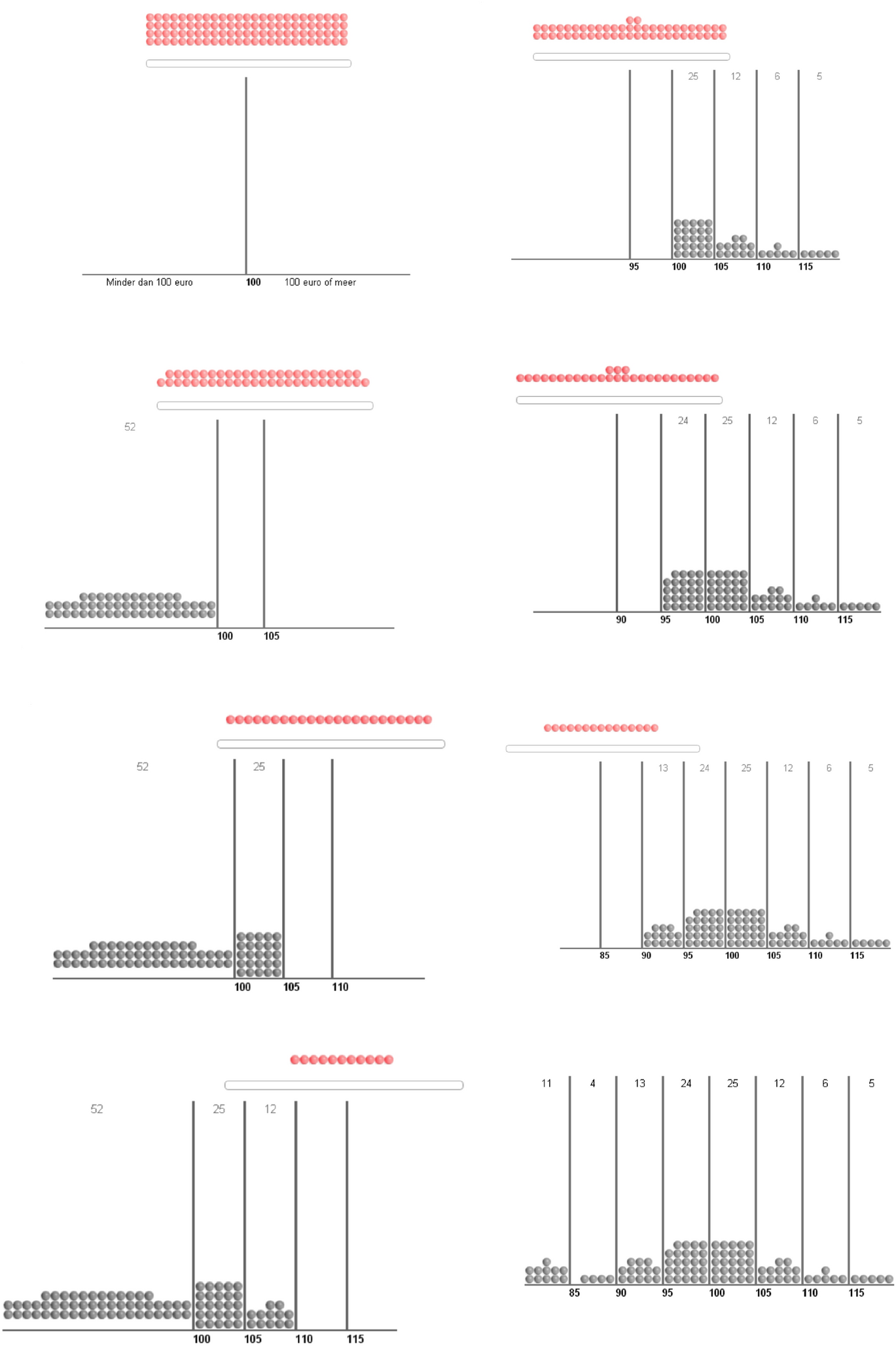
Fig. 3 Iterative expectations interface August 2013.
Source: LISS Panel. The figure shows step 1 to 8 (1 to 4 in the left column, 5 to 8 in the right column) of the iterative procedure used to elicit expectations in August 2013. Respondents could use the slider at the top of the screen to distribute balls from left to right. The red balls above show the remaining balls. The 6 interior bins covered intervals of €5 each. The outer bins were open. The light gray numbers at the top show the number of balls within each bin
In March 2014, respondents were asked whether they would like to adjust their expectations for both assets. To this end, they were first informed about the current value of the asset under consideration. Afterwards, a slightly adapted version of the expectations interface used in August 2013 was presented. Two aspects were changed: For one, instead of having to start entirely anew, the interface was now preset to the distribution of beliefs elicited in August 2013. Second, respondents could use + and − signs below each bin to increase or decrease the number of balls within. Figure 4 shows the interface in March 2014.
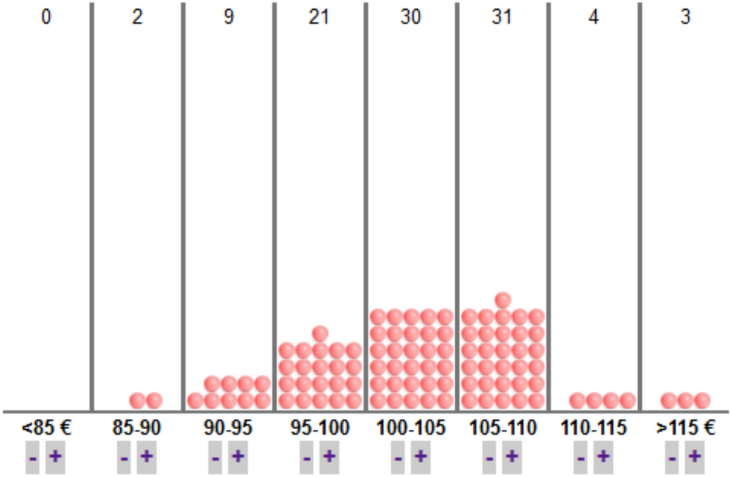
Fig. 4 Expectations interface March 2014.
Source: LISS Panel. The figure shows the interface that allowed respondents to adjust their expectations in March 2014. The 6 interior bins covered intervals of €5 each. The outer bins were open. The + and − signs below each bin could be used to adjust the number of balls within the bin. The numbers at the top show the number of balls within each bin
A.3 Distribution of balls
Figure 5 plots the historical distribution of (inflation-adjusted) AEX returns (left panel) and Philips (right panel) alongside the average probabilities expected by our sample respondents. For both assets, respondents consider returns at both ends of the provided spectrum, i.e., in excess of
 as well as below
 , to be less likely than what has historically been observed. Figure 6 replicates the figure for the second belief elicitation in March 2014. Subjects shifted on average some probability mass to the bins indicating more positive returns.
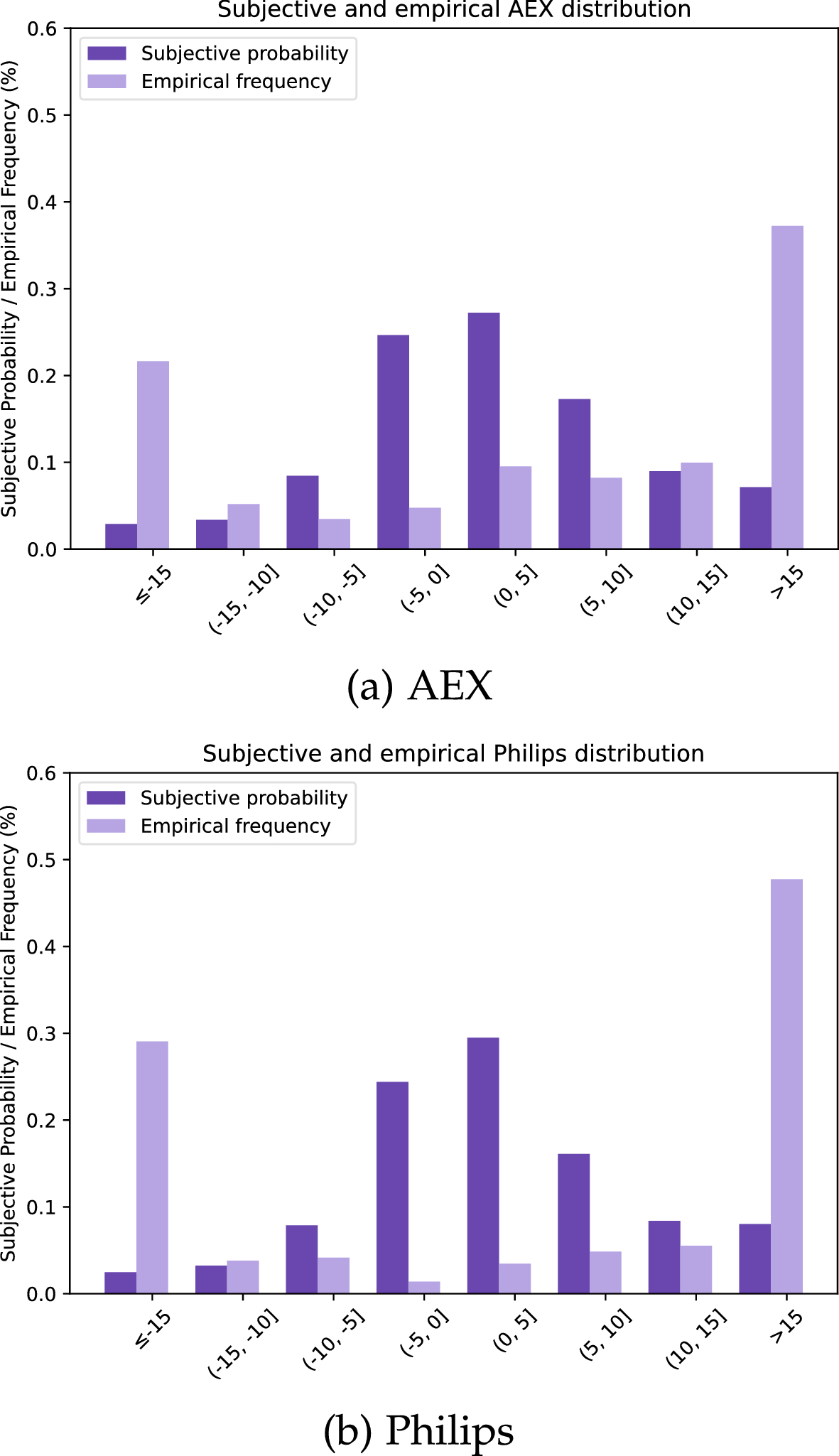
Fig. 5 Expected and historical distribution of AEX and Philips.
Sources: LISS panel and own calculations
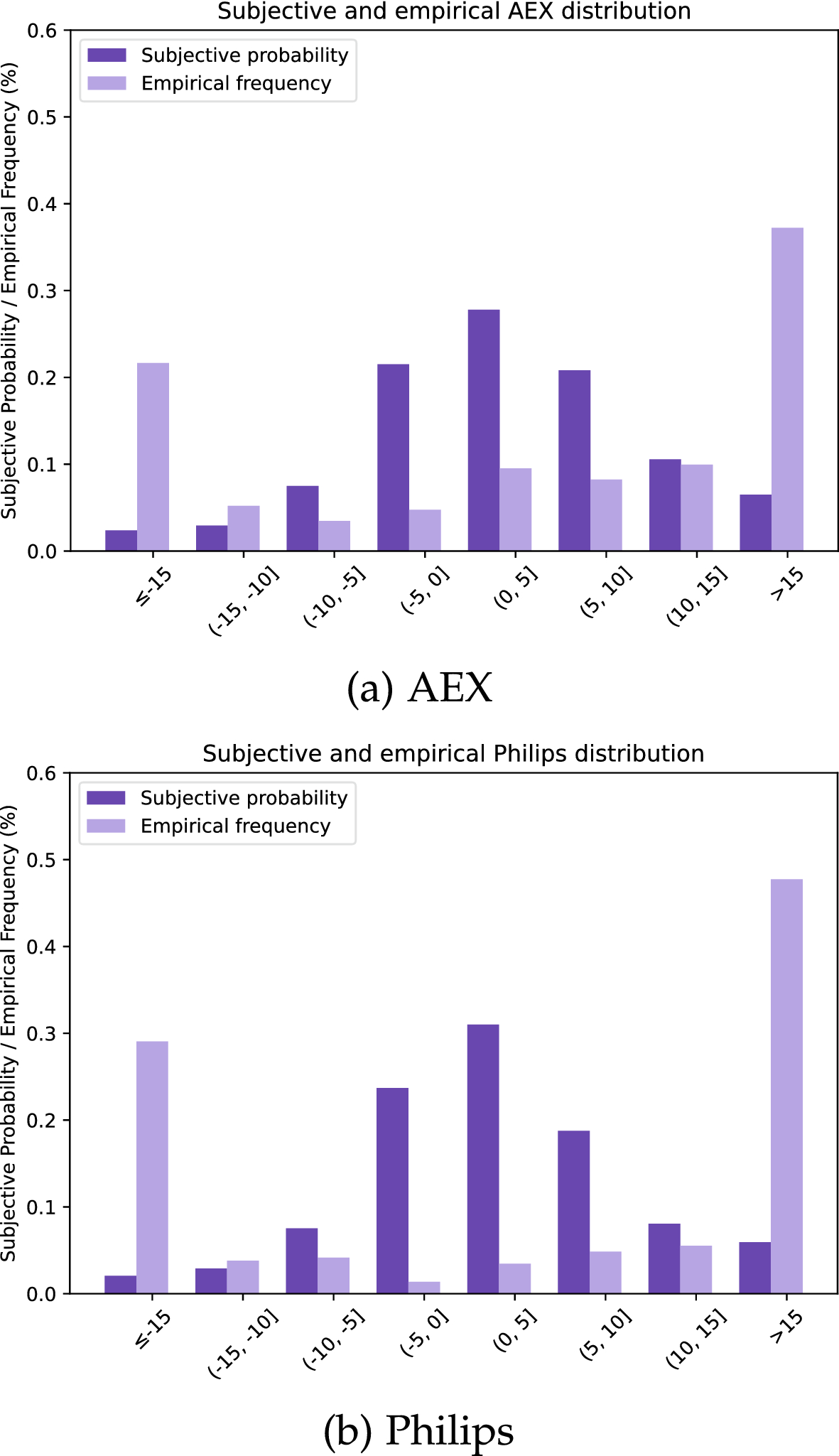
Fig. 6 Expected and historical distribution of AEX and Philips—second elicitation.
Sources: LISS panel and own calculations
A.4 Point estimates for the return of the savings account
In September 2013, point estimates for the return of the savings account were elicited using the following task (translated from Dutch):
Now consider a savings account with a Dutch bank. Suppose you put 100 euros into such an account (details). In about 1 year, you will have the following sum of money:
value in a year = €100 + (potential interest revenue).
How much do you expect the amount of 100 in a standard bank account to be worth in a year? Enter the amount in euros.
When clicking on details, respondents were presented with the description provided for the savings account shown in Sect. A.1 of this appendix. For all of our analyses we winsorize the point estimates at their 5% and 95% quantiles (Fig. 7).
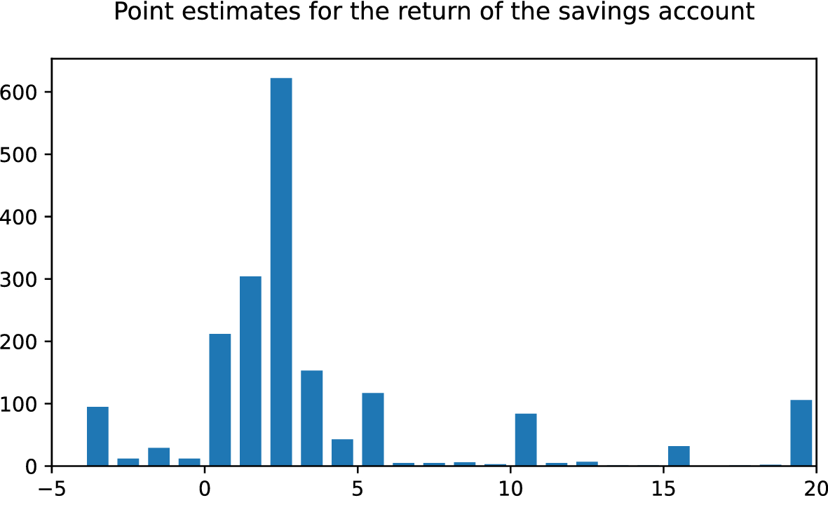
Fig. 7 Distribution of point estimates for the return of the savings account.
Source: LISS Panel. The figure shows the distribution of point estimates for the return of the savings account
A.5 Portfolio choice experiment
A.5.1 Portfolio interface
Figure 8 shows the interface of the portfolio choice experiment in September 2013. The three columns in the figure show the €-shares (in integers) allocated to individual portfolio positions. Respondents could shift the grey controls in each column up and down to increase or reduce the share invested into a given position. “Beleggingsfonds” is the AEX index fund, “Aandelen Philips” is Philips, and “Banktegoed” is the savings account. To the right of the screen respondents saw how much money was currently allocated across the portfolio in total (“Totaal”). They could only proceed with the survey once this value was exactly equal to 100.
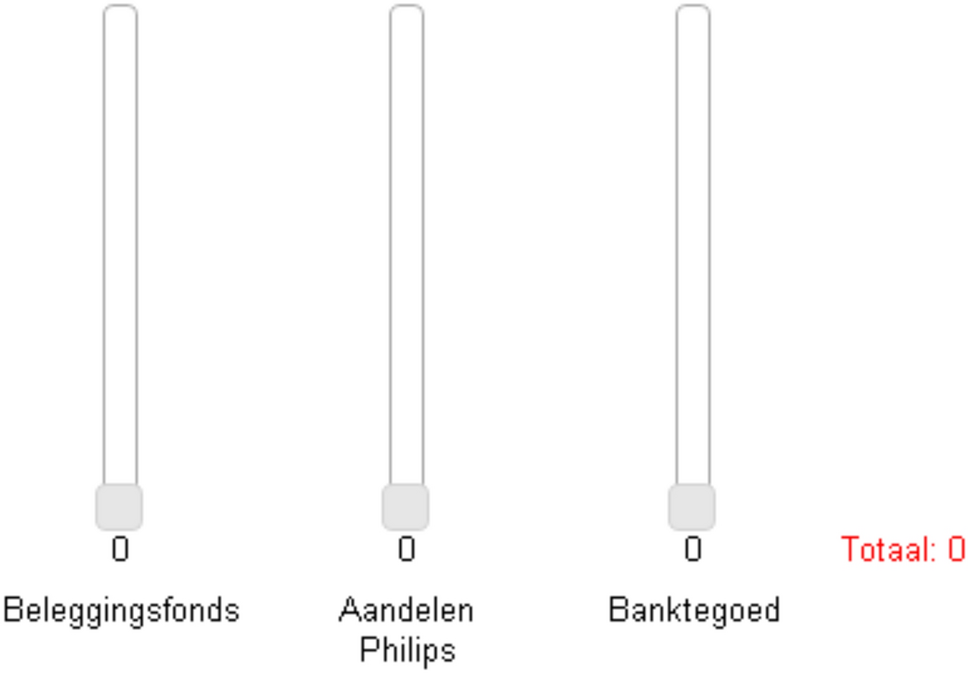
Fig. 8 Portfolio interface September 2013.
Source: LISS Panel. The figure shows the graphical interface of the investment experiment in September 2013. Respondents could move the sliders up and down to allocate a total of €100 among an AEX index fund (“Beleggingsfonds”), shares of Philips (“Aandelen Philips”), and a savings account (“Banktegoed”). “Totaal” indicates the aggregate value of the current portfolio composition
In March 2014, respondents were asked to revisit their portfolio decisions. Again, a graphical interface was employed (Fig. 9). This time, however, respondents did not start out with an empty portfolio as in September 2013. Instead, the interface was preset to the value of the initially selected portfolio, adjusted for intermittent returns between September 2013 and March 2014. Thus, the composition presented was different from the one respondents had originally chosen. Figure 9, for example, contains a portfolio that has appreciated in value and is now worth a total of €106. Respondents were asked to move the sliders to change their portfolios’ compositions. They could proceed with the survey only in case the full current value of the portfolio had been distributed.
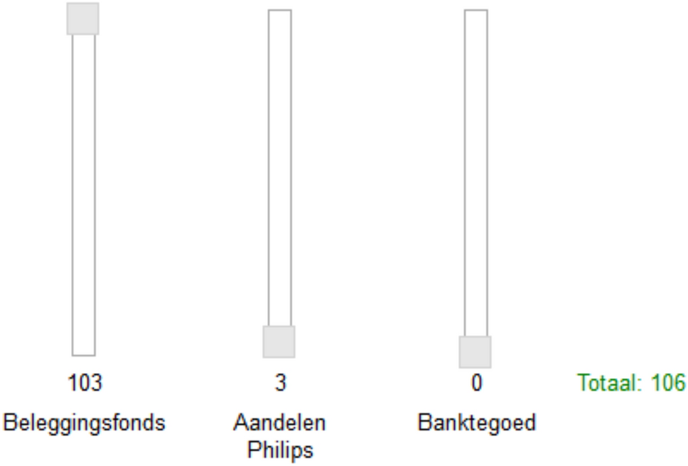
Fig. 9 Portfolio interface March 2014.
Source: LISS Panel. The figure shows the graphical interface of the investment experiment in March 2014. The sliders were initially set to the composition of a respondent’s portfolio after the value of individual assets as well as the portfolio’s total value were adjusted for returns between September 2013 and March 2014. Respondents could move the sliders up and down to reallocate the new total portfolio value among the AEX index fund (“Beleggingsfonds”), shares of Philips N.V. (“Aandelen Philips”), and the savings account (“Banktegoed”). The depicted example shows a portfolio that has increased in value from €100 to €106
A.5.2 Portfolio share descriptives
Table 4 presents descriptive statistics for individual portfolio shares in August 2013 and March 2014 (after rebalancing).
Table 4 Portfolio descriptives.
Sources: LISS panel and own calculations
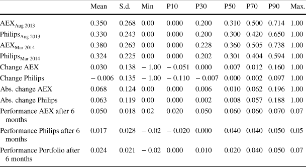
|
Mean |
S.d. |
Min |
P10 |
P30 |
P50 |
P70 |
P90 |
Max. |
|
|---|---|---|---|---|---|---|---|---|---|
|
|
0.350 |
0.268 |
0.00 |
0.000 |
0.200 |
0.310 |
0.500 |
0.714 |
1.00 |
|
|
0.330 |
0.243 |
0.00 |
0.000 |
0.200 |
0.300 |
0.420 |
0.650 |
1.00 |
|
|
0.380 |
0.263 |
0.00 |
0.000 |
0.228 |
0.360 |
0.505 |
0.738 |
1.00 |
|
|
0.324 |
0.225 |
0.00 |
0.000 |
0.202 |
0.301 |
0.404 |
0.594 |
1.00 |
|
Change AEX |
0.030 |
0.138 |
− 1.00 |
− 0.051 |
0.000 |
0.007 |
0.012 |
0.160 |
1.00 |
|
Change Philips |
− 0.006 |
0.135 |
− 1.00 |
− 0.110 |
− 0.007 |
0.000 |
0.002 |
0.097 |
1.00 |
|
Abs. change AEX |
0.068 |
0.124 |
0.00 |
0.000 |
0.006 |
0.010 |
0.062 |
0.196 |
1.00 |
|
Abs. change Philips |
0.063 |
0.119 |
0.00 |
0.000 |
0.002 |
0.008 |
0.057 |
0.188 |
1.00 |
|
Performance AEX after 6 months |
0.050 |
0.018 |
0.02 |
0.020 |
0.050 |
0.060 |
0.060 |
0.070 |
0.07 |
|
Performance Philips after 6 months |
0.017 |
0.028 |
− 0.02 |
− 0.020 |
0.000 |
0.040 |
0.040 |
0.050 |
0.05 |
|
Performance Portfolio after 6 months |
0.024 |
0.021 |
− 0.02 |
0.000 |
0.010 |
0.020 |
0.040 |
0.050 |
0.07 |


The table shows descriptives for individual portfolio shares in August 2013 and March 2014 and descriptives of the performance of the AEX, Philips, and the total portfolios after 6 months
The left panel of Fig. 10 shows the distribution of respondents’ portfolio compositions in September 2013. Each point in the simplex is a bivariate kernel density estimate for varying portfolio shares invested into the AEX (x-axis) and Philips (y-axis) in September 2013. In the right panel, we show similarly constructed kernel density estimates for the changes in portfolio compositions between September 2013 and March 2014, conditional on respondents actively changing at least one component of their portfolios.

Fig. 10 Distribution of portfolio compositions.
Source: LISS Panel and own calculations. The figure shows estimates of the distribution of respondents’ portfolio compositions in September 2013 (left panel) and of the distribution of changes in these compositions in March 2014 (right panel). Each point in the plot corresponds to a bivariate kernel density estimate for given shares invested into the AEX index fund (x-axis) and Philips (y-axis). The distance between each point in the left panel and the hypotenuse corresponds to the share in the savings account. In the right panel, the change in the share of the savings account corresponds to the negative sum of the changes in AEX and Philips. Darker areas contain higher density in both panels
A.5.3 Portfolio value after 1 year
Figure 11 shows the distribution of portfolio values after 1 year.
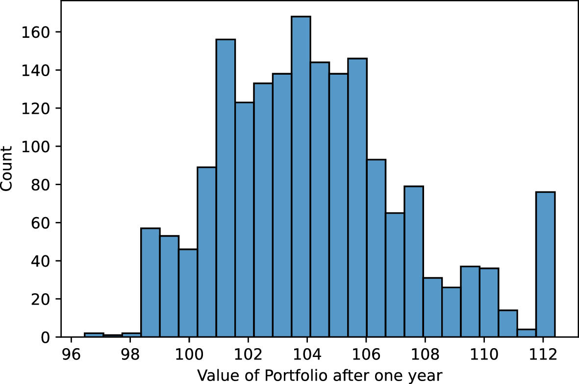
Fig. 11 Distribution of portfolio value after 1 year.
Sources: LISS panel and own calculations
A.6 Sociodemographics
We construct a range of sociodemographic control variables. Part of the experimental instructions was that the financial decision maker of the household should fill in the questionnaire.
Education. LISS collects information on respondents’ educational attainment. We create an indicator, “High education”, that is 1 for respondents who report either a university degree or higher vocational education, and 0 otherwise.
Age. We use LISS’s data on birthyears to create a set of indicator variables for age groups (31 to 50, 51 to 65, and for respondents older than 65).
Gender. We create a binary variable for gender, “Female”, that is 1 in case the respondent is female.
Marital status. Using LISS’s data on the current marital status, we create a variable, “Married”, equaling 1 in case the respondent reports currently being married, and 0 otherwise.
Having children. LISS collects data on the number of children. “Has children” is 1 for all respondents reporting more than 0 children.
Financial wealth. LISS collects detailed information on respondents’ financial assets. We use this data to obtain an estimate for the value of a respondent’s portfolio. To this end, we sum the amounts the respondent reports holding as investments and those in the bank. We set negative amounts of the latter to 0.
For each category of asset, respondents are allowed to provide either continuous or interval statements. Calculating continuous portfolio values requires dealing with the categorical answers. We do this by replacing each interval with its midpoint. For example, if a respondent reports “€7,500 to €10,000” in some category, we replace this answer by the interval’s midpoint, €8,750. We always use the most detailed level of available information. In case a respondent reports values for the aggregate investment category as well as for its subcategories (stocks, funds, and other investments), we use the more detailed data. In case detailed data is not available, we use the answer to the aggregate question.
Based on the resulting estimate, we create indicators for “Financial wealth
 (€10,000, €30,000)” and “Financial wealth
 (€30,000,
 )”. For respondents preferring not to answer the relevant questions we create one more binary variable, “Financial wealth missing”.
Net household income. Using LISS’s information, we categorize households by their net income. For those with income in excess of €2,500, which is the median income of households providing an answer to the income question, we create the variable “Net income > €2,500”. We also create an indicator for households with missing values for income (
 of the sample), “Net income missing”.
Table 5 breaks down the sample in terms of those variables.
Table 5 Sample description.
Sources: LISS panel/own calculations
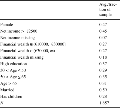
|
Avg./fraction of sample |
|
|---|---|
|
Female |
0.47 |
|
Net income > €2500 |
0.45 |
|
Net income missing |
0.07 |
|
Financial wealth
|
0.27 |
|
Financial wealth
|
0.27 |
|
Financial wealth missing |
0.18 |
|
High education |
0.37 |
|
30 < Age
|
0.29 |
|
50 < Age
|
0.35 |
|
Age > 65 |
0.31 |
|
Married |
0.59 |
|
Has children |
0.28 |
|
N |
1,857 |


The table shows the fractions of our sample that belong to different sociodemographic groups
A.7 Risk aversion
In September 2013, respondents’ aversion to risk was measured. The variable we used in our analyses was composed of three different measures, two based on respondents’ self-assessments and one quantitative measure. For our analyses, we standardize each of the measures and take their average as our proxy for a respondent’s aversion to risk.
Risk questions. The risk questions relied on variants of those developed for the “Preference Survey Module” of Falk et al. (Reference Falk, Becker, Dohmen, Huffman and Sunde2016). These questions were explicitly designed to measure economic preference parameters in large-scale surveys like ours. To validate them, Dohmen et al. (Reference Dohmen, Falk, Huffman, Sunde, Schupp and Wagner2011) show that they are predictive of behavior in experiments as well as in risky situations in the field, including the decision to participate in the stock market. Respondents were asked both for their willingness to take risks in general as well as in financial matters:
Different people have different opinions and characteristics. We are interested in how you describe yourself. In general, to what extent are you willing to take risks? You can answer this question by clicking somewhere on the slider (0–10).
And, in general, to what extent are you willing to take risks in financial matters? You can answer this question by clicking somewhere on the slider (0–10).
Figure 13 shows that respondents in the sample are very heterogeneous with respect to their risk preferences.
Risk lottery. In addition to the qualitative measures, a quantitative measure of risk aversion was constructed. To derive this measure, respondents were asked a series of interdependent hypothetical binary lottery choices. In each of five consecutive rounds, this so called “staircase procedure” asked respondents to decide between a safe payment and a lottery. The lottery was fixed throughout the rounds, every time offering a 50/50 chance to win €300 or nothing. The safe payment, however, varied. Depending on whether the respondent decided to accept the lottery in the previous round or not, the safe payment offered in the next question would either increase (upon acceptance of the lottery) or decrease (upon its rejection).
For instance, the first round started with a safe payment of €160. If the respondent chose the lottery, the safe payment was increased to €240 in the next round. If the safe payment was chosen, the safe amount was consecutively reduced to €80. Ultimately, each respondent arrived at one of 32 possible outcomes, which were evenly spaced between 0 and €320. In essence, the procedure allows us to zoom in on a respondent’s certainty equivalent. To facilitate comprehension of the lottery, each round was accompanied by a graphical representation of the choice (see Fig. 12).
Figure 13 shows that most subjects end up with estimated certainty equivalents below €160, indicating risk averse behavior.

Fig. 12 Graphical illustration of hypothetical lottery choice.
Sources: LISS panel and own calculations. The figure shows the visual interface accompanying one of the lottery decisions
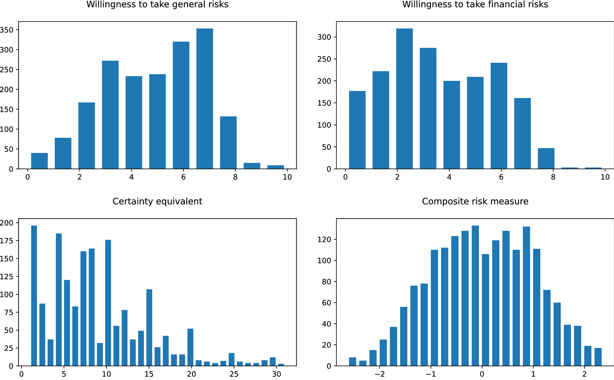
Fig. 13 Distribution of risk aversion components and aggregate variable.
Sources: LISS panel and own calculations. The figure shows the distribution of individual components of our composite risk aversion measure as well as the distribution of the measure itself


 Open access