


Introduction
The role of the Antarctic in the global climate system has long been recognized. The Southern Ocean is an important site of enhanced primary productivity and carbon dioxide uptake; Antarctic Bottom Water (AABW) ventilates the lower kilometre of all the major ocean basins. The Ross Sea contributes approximately half of the 10 Sv (1 Sv = 106 m3 s-1) of AABW production (Orsi et al. 1999); the region is also important to the issues of ice mass balance and potential sea-level rise. The AABW has experienced warming, freshening and volume loss (Purkey & Johnson Reference Purkey and Johnson2013) and, at a more regional scale, water masses in the Ross Sea over the past several decades have freshened (Jacobs et al. Reference Jacobs, Giulivi and Mele2002, Fusco et al. Reference Fusco, Budillon and Spezie2009, Jacobs & Giulivi Reference Jacobs and Giulivi2010). However, recent observations (2014 to present) suggest that High-Salinity Shelf Water (HSSW) is becoming more saline (Castagno et al. Reference Castagno, Capozzi, DiTullio, Falco, Fusco and Rintoul2019). The temporal trends in the HSSW salinity, both the long-term freshening and more recent increase, are focusing attention on the dynamics of this region under climate change forcing.
HSSW, a key constituent in the Ross Sea contribution to AABW (Gordon et al. Reference Gordon, Huber and Busecke2015), is formed in the western Ross Sea within the Ross Ice Shelf and Terra Nova Bay (TNB) polynyas. The latter, located in TNB (Fig. 1) on the coast of Victoria Land, is a coastal latent heat polynya (Bromwich & Kurtz Reference Bromwich and Kurtz1982, Reference Bromwich and Kurtz1984, Martin et al. Reference Martin, Drucker and Kwok2007, Fusco et al. Reference Fusco, Budillon and Spezie2009, Cassano et al. Reference Cassano, Maslanik, Zappa, Gordon, Cullather and Knuth2010). The TNB polynya contributes 40–80 km3 in ice volume production annually (Fusco et al. Reference Fusco, Budillon and Spezie2009, Kern Reference Kern2009, Tamura et al. Reference Tamura2016) over an average 1300 km2 area (Kurtz & Bromwich Reference Kurtz and Bromwich1985). In comparison, the Ross Sea polynya has contributed 300–600 km3 yearly from the early 1990s to the late 2000s over an area of ~29,000 km2 (Comiso et al. Reference Comiso, Kwok, Martin and Gordon2011, Drucker et al. Reference Drucker, Martin and Kwok2011). While the net ice production in the TNB polynya is < 20% of that in the Ross Sea polynya, the more intense ice production rate in TNB and the higher-salinity surface waters found there produce the saltiest and densest shelf water in the Ross Sea (Budillon & Spezie Reference Budillon and Spezie2000, Rusciano et al. Reference Rusciano, Budillon, Fusco and Spezie2013).
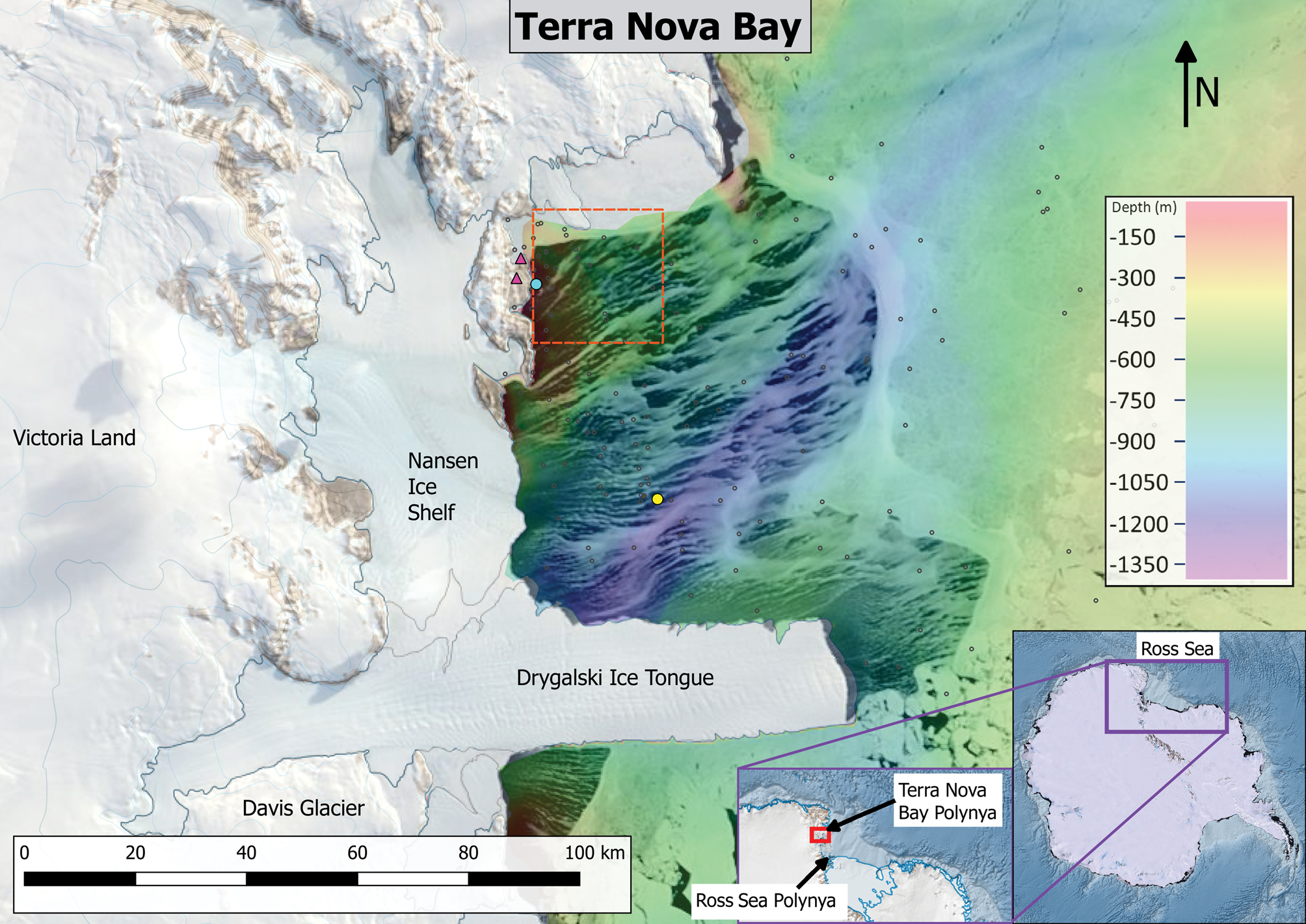
Fig. 1. MODIS Terra visible satellite image of the Terra Nova Bay polynya with 250 m resolution taken on 5 October 2007. Automatic weather stations Eneide and Rita are marked by the two magenta triangles near the cyan circle denoting Mooring L. Mooring D is denoted by the yellow circle. Locations of the conductivity-temperature-depth profiles used in these analyses are shown by small open circles. Bathymetry in Terra Nova Bay is shown, with cooler colours indicating greater water depths. The red dashed box delineates the geographical area where the open-water fraction is determined using Advanced Microwave Scanning Radiometer - Earth Observing System (AMSR-E) satellite data.
The TNB polynya is forced by persistent katabatic winds from the East Antarctic Ice Sheet and sheltered from sea-ice advection from the south by the Drygalski Ice Tongue (Bromwich & Kurtz Reference Bromwich and Kurtz1984), which also provides a control on the maximum areal extent of the ice-free area. These strong winds create a ‘sea-ice factory’, exporting ice seaward and maintaining open water for further ice formation and salt rejection into the water column, which is the primary mechanism in the formation of HSSW (Comiso et al. Reference Comiso, Kwok, Martin and Gordon2011). Hydrographic studies (Budillon & Spezie Reference Budillon and Spezie2000, Budillon et al. Reference Budillon, Pacciaroni, Cozzi, Rivaro, Catalano, Ianni and Cantoni2003, Gordon et al. Reference Gordon, Orsi, Muench, Huber, Zambianchi and Visbeck2009, Orsi & Wiederwohl Reference Orsi and Wiederwohl2009) that have analysed the physical properties of the dense bottom water within the Ross Sea reveal a clear salinity gradient emanating from the TNB polynya associated with HSSW production. A series of summer oceanographic ship-based surveys coupled with two year-round ocean moorings operated by the Italian ‘Climatic Long-Term Interactions for the Mass-balance in Antarctica’ (CLIMA) (Fusco et al. Reference Fusco, Budillon and Spezie2009, Budillon et al. Reference Budillon, Castagno, Aliani, Spezie and Padman2011) and ‘Terra Nova Bay Experiment’ (T-Rex) (Rusciano et al. Reference Rusciano, Budillon, Fusco and Spezie2013, Sansiviero et al. Reference Sansiviero, Morales Maqueda, Fusco, Aulicino, Flocco and Budillon2017) projects provide a baseline understanding of the oceanographic conditions of the TNB region.
The potential temperature/salinity (θ/S) relationship, derived predominantly from high-resolution conductivity-temperature-depth (CTD) data collected from 1984 to 2004 (Fig. 2), reveals the colder, saltier water types found in TNB and their changes over time. Four major water masses can be found within TNB: Modified Circumpolar Deep Water (mCDW), Ice Shelf Water (ISW), Antarctic Surface Water (ASW) and HSSW. The relatively warm (> -1°C) mCDW, drawn from the Circumpolar Deep Water (CDW), spreads into the Ross Sea (Orsi & Wiederwohl Reference Orsi and Wiederwohl2009, see their fig. 2); note that the mCDW in Fig. 2 here is not visible due to the restricted temperature range focusing on the near-freezing point water. ISW, emanating from below the glacial ice shelves, displays temperatures well below the surface freezing line in a series of cold excursions spanning the salinity range of 34.7 to 34.84 in Fig. 2. ISW salinity can be close to that of its HSSW precursor, as ISW is modified by basal melting during its time under the glacial shelves. The salinity of HSSW (θ = -1.85°C, S > 34.7; Orsi & Wiederwohl Reference Orsi and Wiederwohl2009, Budillon et al. Reference Budillon, Castagno, Aliani, Spezie and Padman2011, Rusciano et al. Reference Rusciano, Budillon, Fusco and Spezie2013) can approach 35.0. During the summer, the comparatively warm, low-salinity ASW caps the water column.

Fig. 2. Historical θ/S relationship in Terra Nova Bay from summer conductivity-temperature-depth profiles collected between 1984 and 2004. The 1 atm pressure freezing point of saltwater is indicated by the dashed blue line. The Ice Shelf Water (ISW; Jacobs Reference Jacobs2004) occurs at temperatures below the dashed blue line. The saline High Salinity Shelf Water (HSSW) is found at temperatures near the freezing point with salinity > 34.7. The long-term salinity changes are visible at the surface freezing point (HSSW) and below the surface freezing point (ISW).
Cappelletti et al. (Reference Cappelletti, Picco and Peluso2010), using data collected from 5 February 2000 to 16 January 2001 from both CLIMA moorings L and D (Fig. 1), demonstrated a strong barotropic component to the circulation within TNB, which is cyclonic (clockwise in the Southern Hemisphere) with a seasonally varying surface-intensified baroclinic flow. Once formed, HSSW may take two paths out of TNB: to the south, where it may circulate under the Ross Ice Shelf resulting in ISW; or to the north, where it is exported at the shelf break and becomes part of the Ross Sea contribution to AABW (Budillon & Spezie Reference Budillon and Spezie2000, Buffoni et al. Reference Buffoni, Cappelletti and Picco2002, Fusco et al. Reference Fusco, Budillon and Spezie2009, Cappelletti et al. Reference Cappelletti, Picco and Peluso2010, Gordon et al. Reference Gordon, Huber and Busecke2015). The offshore Mooring D has been used in several studies of the surface heat flux (Fusco et al. Reference Fusco, Budillon and Spezie2009) and relationship between wind field, salinity and polynya area (or open water percentage) (Kern & Aliani Reference Kern and Aliani2011, Rusciano et al. Reference Rusciano, Budillon, Fusco and Spezie2013).
In this study, we quantify the relationship between the HSSW salinity characteristics and the open-water fraction within the TNB polynya, the wind speeds measured at land-based automatic weather stations (AWS) and the subsurface currents in the region.
Prior efforts in modelling the polynya's response to atmospheric forcing have focused more on areal extent, whether analytically (Pease Reference Pease1987, Ou Reference Ou1988) or numerically (Van Woert Reference Van Woert, Spezie and Manzella1999). Because we are particularly interested in the formation of HSSW, we adopt the vertical one-dimensional model (Price-Weller-Pinkel (PWP); Price et al. Reference Price, Weller and Pinkel1986). In particular, we investigate how much effect the strength of the low-salinity summer cap has on the amount of HSSW formed, as well as the timing of the initiation of convection. We also hope to gain further insight into the timing of expansion/contraction events, salinity bursts and katabatic vs synoptic winds.
Data and methods
Mooring
Temperature, salinity, pressure, and current speed and direction were obtained from CLIMA Mooring L, shown in Fig. 1. The near-shore mooring, deployed in 2000, 2001, 2003 and 2007 in ~148 m water depths, is the focus of our investigation of the salinity response of the TNB polynya. The 2007 record was the most complete in terms of data quality and availability at both the near-surface and the bottom instruments. That year, Mooring L was deployed at 74°44.6048′S, 164°08.3916′E and instrumented with an Aanderaa recording current meter model RCM7 at 31 m, a Seabird model SBE37 Microcat at 30 m and an Aanderaa WLR7 water-level recorder at 145 m. Velocity data were reported with 30 min resolution and salinity and temperature with 10 min resolution. The accuracy of the current meters is ± 1 cm s-1 and ± 5° for individual measurements of speed and direction, respectively. Castagno et al. (Reference Castagno, Falco, Dinniman, Spezie and Budillon2017) suggest the high-energy environment in the western Ross Sea allows for the neglect of possible systematic errors at speeds < ± 1 cm s-1. The SBE37 Microcat has a temperature accuracy and resolution of ± 0.002°C and 0.0001°C, respectively, and a conductivity accuracy and resolution of ± 0.003 and 0.0001 mS cm-1, respectively. The accuracy of the Microcat sensor was verified by comparison with CTD casts before and after deployments. The WLR7 water-level recorder has a temperature accuracy and resolution of ± 0.1°C and 0.04°C, respectively, and a conductivity accuracy and resolution of 0.25 mmho cm-1 and 0.1% of the range, respectively.
Satellite
A time series of open-water fraction within the polynya was obtained from the Advanced Microwave Scanning Radiometer - Earth Observing System (AMSR-E) satellite-based sea-ice concentrations calculated daily in near-real time (2002–2011) (data are publicly available at http://www.iup.uni-bremen.de/seaice/amsredata/asi_daygrid_swath/l1a/s6250/). The surface brightness imagery, from which the sea-ice concentration is calculated, has a spatial resolution of 6.25 km, daily temporal resolution and returns good data during overcast periods. Examination of the metadata indicates that the overflight time in the Ross Sea region is approximately 1230 h, with a variability of less than half an hour. The Arctic Radiation and Turbulence Interaction Study Sea Ice (ASI) algorithm used in this product has been described and validated by shipboard observations and comparisons with other remote imagery in both the Arctic and Antarctic regions (Spreen et al. Reference Spreen, Kaleschke and Heygster2008). For this study, we selected a 4 × 4 locus of pixels (6.25 km resolution, or ~39 km2 per pixel) in the area of Mooring L in the north-west corner of TNB to represent local conditions (see bounding box in Fig. 1). Here, the fraction of open water is calculated as the ratio of open water area to the total area within this north-west corner (‘open-water fraction’). The open-water fraction in this region was highly correlated with that in the larger TNB except in December and January, when the Mooring L region of interest in the north-west corner of the bay still showed ~50% ice cover.
Meteorological data
Meteorological data have been acquired at the AWS Rita (74°43.5′S, 164°02.0′E, elevation 267 m), providing data with hourly time sampling. Both AWSs are equipped with sensors to measure atmospheric pressure, temperature, relative humidity, wind speed and direction, solar radiation and snow depth. Data and information were obtained from the Osservatorio Meteo-Climatologico Antartico of the Programma Nazionale di Ricerche in Antartide (data publicly available at http://www.climantartide.it). This study employs data from AWS Rita rather than Eneide (74°41′S, 164°05′E, elevation 92 m), as we have long- and short-wave radiation measurements from Rita in 2009. Measurements from the two stations are highly correlated.
One-dimensional vertical model
We adapted the one-dimensional PWP mixed-layer model (Price et al. Reference Price, Weller and Pinkel1986) to incorporate ice formation. The PWP model was chosen because its physics are well documented and understood. A one-dimensional vertical model neglects several important effects in the salinity balance of the TNB polynya, including horizontal advection and mixing, basal melting of ice shelves, irregularities in the regional circulation such as the presence of large icebergs and export of dense water. The model can, however, be instructive in terms of the effects of local preconditioning, convection and variability in wind stress.
The physics of the PWP model have been well described (Price et al. Reference Price, Weller and Pinkel1986) in a variety of settings. Briefly, the temperature and salinity of the top grid point are incremented by applying surface heat, evaporation and precipitation fluxes. Convective adjustment is effected by mixing all layers above a static instability until that instability is removed. At each time step, adjacent model layers are mixed until the gradient Richardson number exceeds the critical 0.25 value. A bulk mixed-layer Richardson number condition is also required to determine the depth of the mixed layer. Once mixing has been accomplished, surface stresses are applied to step the velocity profile forward in time. Here, we focus on the mixed-layer depth and observed salinity evolution.
Atmospheric forcing was adopted from the 2007 observations at AWS Rita, with reported shortwave radiation, wind speed, temperature and relative humidity averaged to 30 min resolution. Supplemental measurements of longwave (Kipp and Zonen model CGR4) and shortwave (Kipp and Zonen model CMP22) radiation were obtained at AWS Rita by the Lamont-Doherty Earth Observatory (LDEO) between 28 January and 12 December 2009 (data are publicly available on Columbia Academic Commons at https://doi.org/10.7916/D8805F2P). The calculated heat flux is applied at the temperature T(z,t) at the top grid point (ocean surface, z = 0 m) at time step tn +1:
 $$T( {0, \;n + 1} ) = T( {0, \;n} ) + \displaystyle{{( {q_ia( 1 ) -q_o} ) dt} \over {\rho ( 1 ) c_{\,pw}dz\;}}$$
where dt is the time step, dz is the vertical grid resolution, ρ is the seawater density, cpw is the heat capacity of seawater, qi is the incoming solar radiation, ρ(1) is the ocean surface seawater density, a(1) is the absorbance of the incoming solar radiation at the first grid point and qo is the net heat flux out of the ocean due to sensible heat, latent heat and longwave fluxes.
When the sea surface temperature is above the surface freezing point, the original PWP salinity equation is applied. When the sea surface temperature is at or below the surface freezing point, a modified salt flux is applied at the surface. In that case, the salinity S(z,t) at the top grid point (the ocean surface) at time step tn +1 is specified as:
 $$S( {0, \;n + 1} ) = S( {0, \;n} ) -S( {0, \;n} ) P_i\;\displaystyle{{dt} \over {dz}}\;\left[{1-\displaystyle{{S( {0, \;n} ) -S_{ice}} \over {\;1000}}} \right]$$
The ice production rate, Pi, is specified as
 $$P_i = \displaystyle{{( {q_ia( 1 ) -\;q_o} ) } \over {\rho _iL_f}}$$
where ρi is the density of ice, taken to be 916.7 kg m-3, Lf is the latent heat of fusion, taken to be 334 kJ kg-1, and Sice is the salinity of newly formed sea ice, taken to be 10 PSU. A more sophisticated parameterization of Sice = 0.31 Sw (Martin & Kauffman Reference Martin and Kauffman1981) resulted in a 2% difference in the final salinity, where Sw is the salinity of seawater. The ice production rate has units of m s-1 and is scaled by the open-water fraction. Heat flux through the sea ice cover is neglected.
The model is initialized by a suite of 146 temperature and salinity profiles (Fig. 3a & b, respectively) drawn from the historical collection of hydrographic stations in TNB occupied between 1984 and 2004 during the spring and summer months (data are available at https://www.nodc.noaa.gov). Profiles deeper than 200 m, generally drawn from the centre of TNB, are truncated; this may result in anomalously warm and fresh profiles with no real pycnocline. These profiles provide unrealistic but widely varying initial conditions. In order to isolate the effects of the initial stratification, the atmospheric forcing and polynya open-water fraction are identical for each model run, with only the initial stratification varying. The model is incremented forward with a time step, dt, of 30 min and a vertical resolution, dz, of 2 m.

Fig. 3. Profiles of a. salinity and b. temperature used to initialize the Price-Weller-Pinkel model. The red lines show the ensemble average for all a. salinity and b. temperature profiles (see Fig. 1 for the spatial distribution). The depth-integrated temperature relative to the bottom measurement used to quantify the effects of stratification on the onset of High Salinity Shelf Water production is illustrated in c.
Results
The hydrographic observations are necessarily limited to the summer months; the mooring data allow us to examine the evolution of the salinity signature at a given site over the course of an entire year. It is clear from records retrieved from mooring sites in TNB that HSSW is present at depth throughout the year and is visible in the potential temperature/salinity diagram (not shown), appearing near the bottom at 145 m between July and November. The homogeneous water column observed at Mooring L for much of 2007 clearly indicates convection, with salinity values characteristic of HSSW (Fig. 4). Measured velocities at Mooring L are predominantly north-east/south-west (Fig. 4c), probably bathymetry-following given the shallow water in which the mooring is located.

Fig. 4. Comparison of potential a. temperature and b. salinity observed in 2007 at Mooring L. Near-bottom observations (blue traces) of potential temperature and salinity track near-surface values (red traces) for much of the year. A homogeneous water column on Yearday 72 (black line) coincides with reduced ice-free fraction in the polynya. The 31 m velocities in c. were predominantly north-east/south-west; the maximum speed was 49 cm s-1.
In 2007, θ at 30 m increases to -0.48°C in early February 2007, while the θ at 145 m peaks at -1.13°C at 3 weeks later. For most of the summer months, salinity values at the 30 m (near-surface) and 145 m (deep) instruments follow different trends; the deep salinity decreases through February into early March (Yearday 67) to a minimum of ~34.2, while the near-surface salinity begins increasing from its minimum of 33.6 during early February. At Yearday 72, the water column becomes homogeneous (S ≈ 34.3, θ ≈ -1.91), with the near-surface and deep instruments measuring identical values until about December. Salinity continues to increase, reaching a maximum of 34.85 near Yearday 286, reflecting the net effect of winter sea-ice formation. Over the remainder of the year, salinity decreases slightly.
The canonical view of the TNB polynya holds that katabatic winds flowing off the ice sheet bordering TNB drive the forming sea ice seaward, while the Drygalski Ice Tongue protects the embayment from northward sea-ice advection. From approximately Yearday 80 forward, a visual correlation is evident between the 30 m salinity anomaly (calculated by fitting a piece-wise continuous second-order polynomial to the data) and the polynya open-water fraction (Fig. 5a), as well as between the polynya open-water fraction and the 10 m wind speed observed at AWS Rita (Fig. 5b). For example, an increase in salinity is associated with a longer-term increase in open-water fraction within TNB at Yeardays 120, 200 and 220. These days are not inclusive of all events, but they demonstrate a broad response of salinity to polynya opening and closing rather than short-term fluctuations. An increase in the open-water fraction of the polynya precedes a salinity increase; when the polynya begins to close, the salinity decreases after a brief lag, as the net effect of the sea-ice formation evolves. Similarly, associations between 10 m winds exceeding 25 m s-1 (the operational definition of katabatic wind applied by Rusciano et al. Reference Rusciano, Budillon, Fusco and Spezie2013) and increased open-water fractions are evident; for example, on Yeardays 143, 210, 258, 270 and 278 (Fig. 5b). In this case, the polynya open-water fraction increases in concert with periods of sustained katabatic wind activity. The open-water fraction in the embayment suddenly decreases at Yearday 72, coincident with the homogenization of the water column, and it begins to increase again at about Yearday 335. During that time, interaction with the atmosphere through convective and wind-driven mixing drives a well-mixed water column.

Fig. 5. a. Daily averaged de-trended salinity anomalies measured by the 30 m instrument at Mooring L in 2007 and b. 10 m wind speed measured at automatic weather station Rita. In both panels, the Advanced Microwave Scanning Radiometer - Earth Observing System (AMSR-E) polynya open-water fraction is shown in black. Measured wind speeds > 25 m s-1 are marked by red dots in b. A 6 hour moving average has been applied to the wind speed.
A consistent relationship exists between the measured wind speed and size of the polynya opening (or the open-water fraction). The average lag correlation between the two variables from 2000 to 2009 is shown in Fig. 6. A 40-day window was serially applied to each year's wind speed and opening records, shifted in increments of 1 day after the lagged correlation was calculated. Prior to the lagged correlation analysis, all records were normalized to have zero mean and unit variance. The time series of lagged correlations from the individual years were then temporally averaged. In general, both the correlations and lags display periods of intense bursts of activity. The maximum correlation of 0.44 appears at a lag of 1 day in the Yearday 180–220 band. This maximum is set in a long band of correlation of ~0.3 broadly occupying a lag of 0 to -2 days. This correlation appears at about Yearday 90, initially in a fairly broad peak between -6 and -1 days. The peak width contracts and moves to the 1-day lag at Yearday 147. Correlations drop below 0.2 in the band between Yearday 254 and 294. Averaging 8 years of data reduces the variability as well as the maximum correlation. However, inspection of the patterns from individual years shows several that exhibit a longer lag earlier in the year, until about May (autumn), and transitioning to a shorter lag after that time.

Fig. 6. Lag correlation of wind speed measured at automatic weather station Rita and Advanced Microwave Scanning Radiometer - Earth Observing System (AMSR-E)-derived open-water fraction averaged over 2002–2009. Correlations were calculated in 40 day windows starting at Yearday 50 and the eight resulting records were then averaged temporally.
We performed a similar lagged correlation analysis on the salinity, wind speed from AWS Rita and open-water fraction. We selected the near-surface water salinity measurements; while the deeper salinities clearly tracked those at the near surface, the instrument at 145 m did not allow for the resolution of short timescale events. The 90% confidence intervals were estimated via the bootstrap technique. Due to the gap in salinity data between Yeardays 138 and 173 (see Fig. 4b), we estimated correlations based on Yeardays 50–138 and 173–300.
The maximum correlation between daily averaged salinity and the open-water fraction is 0.50 during the latter part of the year (Table I), with the salinity signal lagging the polynya open-water fraction record by 2 days (Fig. 7a). Early in the year, the correlation of -0.32 between salinity and polynya open-water fraction is not significant at the 90% confidence level. For the earlier part of the year, the lagged correlation between hourly averaged salinity and 10 m referenced wind speeds was stronger (Fig. 7b), with a maximum of 0.48 at a lag of almost 6 days. The correlation between wind and salinity in the later part of the year shows a broad maximum of ~0.32 at ~4 days.

Fig. 7. a. Lagged correlation between daily averaged salinity and the open-water fraction of the polynya. b. Lagged correlation between hourly averaged salinity and wind speed measured at automatic weather station Rita.
Table I. Maximum correlation and the lag at the maximum correlation between Mooring L salinity and wind and polynya open-water fraction. Two intervals are specified: before and after the salinity data gap between Yeardays 138 and 173. The correlations are significant at the 90% level (bold) except for the salinity/polynya open-water fraction between Yeardays 50 and 138.

Salinity responds more strongly to wind speed than open-water fraction in the late summer and early autumn. Overturning due to wind mixing in early autumn as the water column is homogenized is a possible mechanism for this observation. Additionally, sea ice may still form while TNB is essentially open, complicating the relationship between salinity and polynya open-water fraction. In the winter, salinity primarily responds to open-water fraction.
The salinity profile evolution of the one-dimensional vertical mixing model is illustrated in Fig. 8. As the mixed layer deepens due to wind mixing, the near-surface salinity is entrained, raising the surface salinity but lowering the mixed layer values. Salt is being redistributed, rather than increasing, as heat is lost to the atmosphere. This stratification due to the summer warm, fresh cap must be removed before the HSSW formation can be directly coupled to the polynya sea-ice formation via brine rejection. Once the surface temperature reaches the freezing point, brine rejection through sea-ice formation induces a steady increase in salinity throughout the mixed layer, and the entire water column becomes homogenized within 2–3 weeks, as observed in the mooring data (Fig. 4). The shallow water column allows mixing to the bottom, dividing the winter into two distinct periods: one that experiences both entrainment and convection and one that is dominated by convection.

Fig. 8. Time evolution of a representative salinity profile in the Price-Weller-Pinkel model. Daily profiles show the deepening of the mixed layer entraining salty water and eroding stratification.
Discussion
The longer lag between the observed salinity and the wind forcing, as compared to the open-water fraction, indicates that ice formation is the mechanism directly forcing the salinity increase: the ice formation lags the wind increase and the water column salinity lags the ice formation. The maximum salinity for a given event occurs after the termination of the katabatic wind event, as sea-ice formation continues to reject brine while the polynya contracts. A 2 day lag between the wind field and the polynya open-water fraction is implied by these results and is consistent with observations by Kurtz and Bromwich (Reference Kurtz and Bromwich1985). It has also been shown that the polynya opening generally begins in the waters closest to the Drygalski Ice Tongue (off the Davis Glacier; see Fig. 1) and spreads northward (Ciappa et al. Reference Ciappa, Pietranera and Budillon2012). Rusciano et al. (Reference Rusciano, Budillon, Fusco and Spezie2013) noted that the polynya opening seems more sensitive to the duration of a katabatic wind event than its intensity. Ou (Reference Ou1988) demonstrated that the polynya is insensitive to high-frequency variability. Responding to the ice formation, the salinity response can be expected to have a more integrative nature rather than responding immediately to the high-frequency changes in the wind field. Ou (Reference Ou1988) also noted that perturbations in air temperature and associated heat loss might be more effective at driving ice-edge responses than the winds.
The record during winter 2007 (Fig. 9a) shows a strong correlation at ~4 days between Yearday 170 and 225, which was strongest after Yearday 190. Subsequently, this trend deteriorates with the maximum correlation shift to ~9 days, a result we hypothesize is not indicative of a systematic relationship. At this time of year, the occurrence of katabatic wind events has greatly weakened. Rusciano et al. (Reference Rusciano, Budillon, Fusco and Spezie2013) noted that the polynya seems to operate at less than full efficiency in terms of sea-ice production over part of the year; our results quantitatively support this effect at a different location within TNB. In addition, Sansiviero et al. (Reference Sansiviero, Morales Maqueda, Fusco, Aulicino, Flocco and Budillon2017) noted that a katabatic wind event was required to open their modelled polynya, while an offshore wind component of 10 m s-1 was able to prevent it from closing. Because salinity values should continue to increase under more moderate wind speeds sustaining an open polynya, a lag between the maximum wind speeds and peak salinity values is to be expected. A reduction in the frequency and intensity of katabatic wind events could further weaken the relationship between the wind speed and salinity.

Fig. 9. Lag correlations of a. salinity anomalies and polynya open-water fraction and b. salinity anomalies and observed wind speed at automatic weather station Rita as a function of time. A 40-day window was applied to the salinity and open-water fraction records and incremented forward by 1 day through the length of the record. The results highlight the temporal variability of the correlation and lead-lag relationship throughout the winter and spring months of 2007.
Earlier in the year, prior to the data gap, which commences at Yearday 138, there is not a definitive strong relationship between the salinity and the polynya open-water fraction (Fig. 9a). A local maximum in the correlation appears at ~3 days in the period between Yeardays 80 and 100. This represents the autumn period when TNB has just started to ice over (compare this to the polynya open-water fraction record in Fig. 5). In 2007, the water column in TNB has become well mixed but has yet to reach its most extreme temperature and salinity values.
One concern is the impact of the non-regular observation times for the ice-cover imagery and how it might impact the correlation with the salinity. Fortunately, as noted earlier, the overflight times in the Ross Sea region are ~1230 h UTC, and we centred the daily average of the salinity measurements at 1200 h. The half- to three-quarter hour difference should have a negligible impact on the correlation between daily averaged salinity observations and the daily ice-cover imagery.
The variability of correlation between the 30 m observed salinity and the wind speed measured at AWS Rita (Fig. 9b) differs from that of the correlation between salinity and the polynya open-water fraction. The maximum correlation (0.5) occurs between Yeardays 75 and 100 (March–April), when TNB is quickly icing over at the beginning of winter. The lag at this time is ~6 days; later in the winter, the relationship between wind and observed salinity weakens and the lag decreases to ~3 days (Fig. 9b). The relationship between salinity and wind appears strongest before the interaction between the polynya and atmospheric forcing becomes fully established. This relationship can be explained by the stronger wind-induced vertical mixing early in winter when thermohaline stratification is still present, which permits the entrainment of saltier deep water into the lower-salinity surface layer before the winter convective mode sets in. The TNB polynya open-water fraction responds to the katabatic wind regime (Kurtz & Bromwich Reference Kurtz and Bromwich1985, Rusciano et al., Reference Rusciano, Budillon, Fusco and Spezie2013) rather than the synoptic winds. Early in the year, the salinity appears to respond more to the synoptic winds while TNB freezes over but before the winter dynamics are fully established.
Kern & Aliani (Reference Kern and Aliani2011) performed a similar analysis of the lag correlations between the polynya area and the salinity measured at Mooring D, located at a depth of 1000 m in the centre of TNB, for the years 1996–1998. In contrast to the results presented here, their work indicated that at Mooring D the time lag lengthened rather than shortened as the winter progressed. In addition, they demonstrated that their lag estimate of 3–4 days was consistent with plausible vertical speeds as the convective plumes descended to the observation depth of 145 m. The longer lag between polynya area and salinity later in the season was explained by the reduced density contrast between the descending convective plume and the ambient waters. Here, we observe a slightly shorter lag (2 days) between salinity and the polynya open-water fraction but at a sensor depth of 30 m, or only 20% of the sensor depth for the Mooring D observations. The deeper water column at Mooring D as opposed to Mooring L suggests that the response to the forcing would require a longer time to penetrate to the sensor depth and thus a longer time lag. The mixed layer can grow much deeper at Mooring D than at Mooring L (which is restricted by the bottom). Furthermore, at the Mooring D location (25.3 km from the coastline along a wind trajectory), the air-sea heat flux is diminished as both the wind stress and the air-sea temperature contrast are attenuated seaward from the coast, leading to a weaker salinity response.
The modelling effort provides little explanation for the timing of the appearance of the salinity signature at depth. PWP's representation of convection results in an instantaneously mixed water column, preventing examination of the contribution of convection to the lag between forcing and salinity. The most obvious result of the model effort is that the modelled salinity increases more strongly than the observed salinity, with a range of 35.15 to 37.16 (mean 35.77 ± 0.28), compared to the 34.72 observed for the Mooring L salinity on Yearday 248. There are several possible explanations for this. As noted earlier, the one-dimensional vertical model neglects several processes that must contribute to the salinity cycling within TNB, including horizontal advection and mixing, the addition of basal meltwater, HSSW export and tidal processes. The use of historical temperature and salinity profiles, measured when HSSW was significantly saltier than it was in 2007, also introduces a tendency towards higher final salinities. We also note that the model does not reproduce the summer melt low-salinity extreme observed at 30 m at Mooring L centred at about Yearday 25, so that even the same salinity increase as that observed would result in a higher final value. Also a possibility is a potential bias in the remote imagery at low ice concentrations (Martin et al. Reference Martin, Drucker, Kwok and Holt2004, Kwok et al. Reference Kwok, Comiso, Martin and Drucker2007), possibly leading to inflated heat fluxes and ice-formation rates.
The ASI algorithm upon which this ice concentration product is based utilizes the 89 GHz channel rather than the lower frequencies employed by the NASA Team and bootstrap algorithms. The 89 GHz channel has higher spatial resolution and increased ability to discriminate the difference between vertical and horizontal polarizations indicative of different kinds of ice and open water. It is, however, more sensitive to water vapour and precipitation, an issue that the ASI algorithm addresses by weather masking provided by the lower-frequency channels.
Ice concentrations from the ASI algorithm have been compared to those from the other two algorithms on large-scale distributions in the Arctic and Antarctic, as well as shipboard observations (Spreen et al. Reference Spreen, Kaleschke and Heygster2008, Heygster et al. Reference Heygster, Weibe, Spreen and Kaleschke2009). There was no significant difference between the three algorithms, although the smaller footprint of the higher-frequency channel used in the ASI algorithm enables better resolution of coastal features and small polynyas, as demonstrated by Martin et al. (Reference Martin, Drucker, Kwok and Holt2005). Spreen et al. (Reference Spreen, Kaleschke and Heygster2005) also demonstrate that the ASI algorithm identifies open water not identified by the bootstrap algorithm with 12.5 km resolution but clearly visible in contemporaneous Moderate Resolution Imaging Spectroradiometer (MODIS) imagery. Finally, a comparison of the ASI algorithm with Polynya Signature Simulation Method (PSSM) ice distributions calculated from Special Sensor Microwave/Imager (SSM/I) imagery (Kern et al. Reference Kern, Spreen, Kaleschke, De La Rosa and Heygster2007) suggests that the ASI algorithm seems to be able to distinguish between continuous thin ice and a mixture of open water and pancake or frazil ice.
There is the possibility that the ASI algorithm overestimates values at low ice concentrations. We compared open-water fractions derived from the ASI algorithm and SSM/I for 2002–2011. The SSM/I record shows a lower bound of ~20% open water, while the AMSR-E open-water fraction does at times approach or reach zero.
Kern et al. (Reference Kern, Spreen, Kaleschke, De La Rosa and Heygster2007) define the polynya open area as the Open Water plus Thin Ice classes from the PSSM; they note that the average ASI concentration in the Thin Ice class is 65%, and they estimate a maximum thickness of 20–25 cm, which is the ice thickness used by Martin et al. (Reference Martin, Drucker, Kwok and Holt2004) to define the extent of the polynya as encompassing the bulk of the heat loss. These values are more generous than the polynya open-water fraction used in this study. We evaluated annual average areas from 2003 to 2010 and the salinity evolution in the PWP model for open areas defined by 0%, 10%, 20%, 30%, 40% and 50% ice concentrations. In these cases, pixels with ice concentrations above the selected threshold were set to zero. The 0% and 10% ice concentration thresholds yielded salinities lower than that measured at Mooring L on Yearday 250 (34.73). A 20% ice concentration threshold best represented the salinities measured at Mooring L on Yearday 250 (34.79); while this threshold is close to the estimate of 25% ice in the open water class of the PSSM of Kern & Aliani (Reference Kern and Aliani2011), it also neglects any horizontal advection, export and mixing of fresher waters. Water-column homogenization in the model occurred in April rather than March. The 50% ice concentration threshold yields a final model salinity of 35.76, which is 1.03 higher than our results. We thus conclude that while a thin-ice bias may contribute to the model's overestimate of the salinity, it is not likely to be the major factor.
While the modelled salinity increases well beyond that observed, it does capture much of the amplitude and behaviour observed at Mooring L. The average over all of the model runs forced by varying initial stratification, shown in Fig. 10 along with the 1 SD variability envelope, captures most of the different polynya events. Moreover, the order 10 day timescale oscillation of salinity linked to the polynya expansion and contraction is apparent in the modelled salinity anomaly (Fig. 10). A 10 day moving average filter has been applied to the observed salinity anomaly, smoothing out the short impulses in the trace and highlighting the broad changes associated with polynya expansion and contraction. Individual runs show different degrees of fidelity to the observed salinity anomaly, particularly after the gap in the salinity observations, which ends on Yearday 175. While the timing is generally well-matched, some events are not well-represented in terms of magnitude (e.g. compare the model ensemble average to the observed salinity peaks at about Yeardays 115 and 200). The compressed range of the salinity variability is due to the inclusion of artificially enhanced variability introduced by including initial profiles from throughout TNB, done purposefully to fully explore the effect of stratification. Restriction to profiles from depths shallower than 250 m results in an average anomaly lower than the ensemble average before Yearday 140 and higher than the ensemble after Yearday 160. The model does capture the pattern of higher-frequency cycles of response to the polynya open-water fraction, which result in a seasonal increase in the salinity as HSSW is produced. The model run that best reproduced the observed salinity cycles yielded a correlation of 0.7 with the 2007 salinity measurements between Yeardays 68 and 136.

Fig. 10. Comparison of observed (black) and ensemble-mean modelled (red) salinity anomalies at 30 m. The red trace envelope shows the 1 SD variability for all model runs. Mean modelled salinity anomalies for all stations with depths < 250 m are shown in blue. A 10 day moving average has been applied to the observed salinity anomalies to yield the green line.
The magnitude of the modelled salinity histories exhibits a lower fidelity to the observed salinity after about Yearday 200, even though the timing is reasonable. This is unsurprising considering the lower correlations between salinity and polynya open-water fraction and salinity and wind shown in Fig. 9 observed later in the year. Katabatic wind events are less frequent later in the winter, and there are changes in correlation sign between the salinity and measured velocities both intra- and inter-annually (Kern & Aliani Reference Kern and Aliani2011). There is a series of short-lived high-salinity bursts in the anomaly record not reproduced by the model. The strongest positive burst at Yearday 200 is a brief transient, and upon visual inspection it coincides with a reversal in the zonal velocity, including some of the strongest zonal speeds measured over the year. The extrema, which occur in the observed salinities near Yearday 220, are not captured by the modelled results, which represent a broad, integrative increase rather than a series of short-lived extrema. Closer examination of the measured salinity reveals those extrema are correlated with the current direction. There are four north/south direction reversals that occur at 2 day intervals, which appear coincident with the salinity extrema. This different behaviour, with no lag, results in a lower correlation with the wind and open-water fraction forcings. The simple wind-driven velocities in the model do not produce these reversals and cannot capture the salinity response to them. Kern & Aliani (Reference Kern and Aliani2011) showed a similar interannual variability in the dependence on circulation and polynya dynamics.
Although the modelled salinity does not completely reflect the observed salinity, it does show similar oscillatory behaviour. An obvious candidate for the mechanism driving those salinity oscillations is the ice production rate corresponding to fluctuations in the polynya open-water fraction. To investigate this further, we randomly chose an initial profile near the Mooring L location at a depth of ~200 m and isolated different atmospheric forcing mechanisms in order to examine their effects. We initially set a baseline run with no wind mixing, a constant wind stress (τx = 0.21 N m-2, τy = -0.04 N m-2, the annual mean measured at AWS Rita in 2007); a constant polynya open-water fraction is set to 0.2 and 0.4; and a smoothly varying net heat flux was meant to allow only seasonal variability, specified by fitting quadratic functions to the net incoming and net outgoing radiation. Following this baseline, one variable was systematically turned on at a time. The baseline cases with constant open-water fractions showed no variability beyond a convex shape produced by a slowing rate of salinity increase (Fig. 11, inset). This change happens at about Yearday 160 for the 0.2 open-water fraction case (Yearday 120 for the 0.4 open-water fraction case) when the mixed layer deepens enough to allow entrainment of waters below the halocline. Once entrainment of the deeper, saltier waters begins, the rate of salinity increase slows, as the lower contrast between the deeper waters and the descending brine plume results in less relative change. The fluctuation of the polynya open-water fraction produces most of the higher-frequency variability, while the net heat flux modulates this effect. The wind stress has no impact on the variability of the modelled salinity, as its effects have already been incorporated in the open-water fraction and net heat flux, both specified as inputs to the PWP model. In the model, the wind stress affects only the horizontal velocities and mixed layer depths, if wind mixing is allowed.

Fig. 11. Salinity anomalies and salinity (inset) at 30 m depth in the process study of the forcing in the Price-Weller-Pinkel model. The baseline case (black, Case 1) specified a constant polynya open-water fraction of 0.4, constant wind stress, no wind mixing and a heat flux record with seasonal variability only. Subsequent model cases allowed one forcing mechanism to vary as observed: the polynya open-water fraction (red, Case 11), the heat flux (blue, Case 2), the wind mixing (yellow, Case 3) and the polynya open-water fraction and heat flux together (cyan, Case 12). Note that the yellow curve perfectly overlays the black.
By utilizing the prescribed polynya open-water fraction, we have built in the effects of wind stress; the lack of prognostic wind stress means that we cannot compare the observed and modelled time lag between wind events and salinity peaks. We can, however, quantify the relationship between the variability in the applied net heat flux and salinity. The final modelled salinity in the 0.4 open-water fraction baseline case was 35.72; allowing the polynya to fluctuate resulted in a lower final salinity of 35.49. Adding the variable heat flux to the constant polynya open-water fraction raised the final salinity to 35.73, while adding the heat flux to the fluctuating polynya open-water fraction resulted in a slightly higher salinity relative to the variable open-water fraction case of 35.50.
The examples with a constant polynya open-water fraction of 0.4 had the highest final salinity but increased more slowly until near the end of June. On Yearday 173, the rate of salinity increase for the variable polynya open-water fraction cases peaked and began to slow; 20 days later, the salinity in the constant polynya open-water fraction cases exceeded the variable open-water fraction cases. Yearday 173 corresponds to the day on which the observed polynya open-water fraction dropped below 0.4 (see Fig. 5); the mean open-water fraction over the next 90 days is 0.23, only exceeding 0.4 for a total of 8 days.
In 2007, the water column reached homogenization at Yearday 72 in concert with a very rapid decrease in the open-water fraction in TNB. A similar timing is noted in the other years for which we have data at Mooring L. As expected, the model results show that the time to reach a uniform water column varies with the degree of initial stratification and the depth of the mixed layer. We quantify this effect using the net heat and freshwater that must be removed before ice production can begin to add salt to the water. Heat loss needs to reduce the surface temperature to the freezing point and the halocline needs to be removed for deeper convection to occur. Depth integrating the differences between the initial profiles of temperature and salinity and their respective bottom measurements (Fig. 3c) accounts for variability in mixed-layer depth and in the depth and intensity of the pycnocline. The time to homogenize the water column is almost linear over the range of depth-integrated salinity difference. The average time is 24 ± 16 days, with a range of 0–168 days. This timing shows much more variability than we observed at Mooring L. We have deliberately maximized the variability in initial conditions by using temperature and salinity profiles taken throughout TNB, rather than ones that represent conditions only at Mooring L. The time for the surface to cool to the freezing point is 44 ± 19 days, with a range of 22–105 days. The time to reach the freezing point has no dependence on the depth-integrated salinity difference, while the time to homogenize after that point is independent of temperature.
This highlights the differing behaviours of the system before and after ice production begins. While heat is being removed from the surface, the water column is stirred, changing the density distribution but not producing HSSW. While the time to reach a completely homogenized water column is not independent of the time necessary to reach the seawater freezing point, the variability is much reduced once the heat has been removed. Once the heat accumulated in the near-surface layer over the short summer season is removed, the heat fluxes are dominated by ice production.
Summary and conclusions
The TNB polynya opening provides a window between the cold polar wind and the water column salinity, including the formation of HSSW. While the katabatic winds force some heat and freshwater loss, brine rejection during sea-ice formation provides the bulk of the salinity increase. The timing of the onset of sea-ice formation and HSSW formation is dictated by the regional environmental conditions, in particular the density contrast between the surface and the HSSW layer. Wind mixing and heat loss first decrease the buoyancy of the surface layer; when sea-ice production removes the density contrast between surface and deep water, the underlying HSSW is eventually injected with altered surface water.
At higher frequencies, the 2007 time series shows polynya development on average during days 1–2, with salinity increasing from day 3 onward. It logically follows that the polynya open-water fraction lags the wind forcing and the salinity response lags the polynya open-water fraction. Additional lag may be due to the time required for mixing.
Through lag correlation analysis on shorter timescales, we have found a more complicated temporal variability of the katabatic winds, polynya open-water fraction and salinity response. The open-water fraction in the bay responds more strongly to the synoptic winds and at a longer lag (4 days) in spring than it does after midwinter. Conversely, the salinity is more closely tied to the polynya open-water fraction during the height of winter and becomes essentially uncorrelated as the katabatic wind events decrease in frequency after July. The salinity response to the wind forcing is best correlated during the autumn (March/April) with a lag of 5 days. Our results show generally shorter lags that increase later in the winter, both observations being in contrast to previous lag correlation analyses at Mooring D.
A one-dimensional vertical model could not reproduce the absolute salinity values measured at Mooring L in 2007 but did capture the order 10–20 day oscillations in salinity that the variations in polynya open-water fraction superimpose on the seasonal increase as continual sea-ice formation produces HSSW. In the model, the time for the 200 m water column to become well mixed depended on the amount of buoyancy that needed to be removed before ice formation could begin. That time reflects the interplay of two regimes: one in which heat loss prepares the water column for ice formation and redistributes salinity and a second stage in which sea-ice production results in a well-mixed water column. In this second stage, heat fluxes are dominated by the heat released in freezing, and our lag correlation analysis suggests that the salinity responds less directly to the wind forcing.
A simple process study in which we isolated forcing mechanisms individually indicated that the open-water fraction of the polynya provides the primary control on the order 10–20 day oscillations superimposed on the increasing salinity. The amplitude of the salinity response is modulated by the heat flux.
Our study shows that the TNB polynya's role in linking the wind forcing and salinity response, as well as the eventual formation of HSSW, evolves over the year. We confirm quantitatively a varying degree of efficiency in the polynya operation, showing the evolution of the strength of correlation between the three parameters and the lag at which those correlations occur.
Acknowledgements
We thank the reviewers for their thoughtful and insightful comments. This is Lamont-Doherty Earth Observatory contribution number 8395.
Author contributions
DALB, CJZ and ALG developed the scientific ideas. DALB and CJZ developed the presentation of and wrote the manuscript. DALB processed the data and ran the models. GB and ALG provided comments on the original manuscript. GB provided the CLIMA Mooring L data.
Financial support
This work was supported by NSF Award Nos. ANT-0739519 and ANT-1341688 to Lamont-Doherty Earth Observatory of Columbia University. Logistical and financial support for CLIMA, MORSea and T-Rex projects was provided by the Italian National Program for Antarctic Research (PNRA- PdR 2009/A2.04, OSS-13 MORSea and T-Rex; 2009/B.09).
Details of data deposit
AMSR-E satellite-based sea-ice concentrations are available at http://www.iup.uni-bremen.de/seaice/amsredata/asi_daygrid_swath/l1a/s6250. Meteorological data for AWS Eneide and Rita are publicly available at http://www.climantartide.it. LDEO radiation data at AWS Rita in 2009 are publicly available on Columbia Academic Commons at https://doi.org/10.7916/D8805F2P. Hydrographic stations in TNB occupied between 1984 and 2004 are available at https://www.nodc.noaa.gov in the World Ocean Database (WOD13), geographical square 3716, Ocean Station Data (OSD) and CTD files.


