


1 Introduction
Two-phase flows are abundant in nature and in industrial applications, where they exhibit many interesting behaviours arising from the interaction between the phases and the different length scales at play (Sundaresan Reference Sundaresan2000; Tenneti & Subramaniam Reference Tenneti and Subramaniam2014; Stone Reference Stone2017). The presence of the second phase can augment or diminish the turbulence characteristics (De Marchis & Milici Reference De Marchis and Milici2016; Eaton & Longmire Reference Eaton, Longmire, Michaelides, Crowe and Schwarzkopf2017; MacKenzie et al. Reference MacKenzie, Soderberg, Swerin and Lundell2018) and change the rheological properties of the fluid (Wylie, Koch & Ladd Reference Wylie, Koch and Ladd2003; Brennen Reference Brennen2005). The phase interactions can also lead to an uneven distribution of particles in the flow (Troutt Reference Troutt2006; Lau & Nathan Reference Lau and Nathan2016) and erosion or dissolution processes (Claudin, Duran & Andreotti Reference Claudin, Duran and Andreotti2017; Ristroph Reference Ristroph2018). The many applications of multiphase flows along with their complex dynamics make developing accurate models challenging and consequential (Tenneti & Subramaniam Reference Tenneti and Subramaniam2014).
One of the parameters to characterize two-phase flows is the Stokes number, which is the ratio of the particle response time to the fluid response time,
 $$\begin{eqnarray}St=\frac{\unicode[STIX]{x1D70F}_{p}}{\unicode[STIX]{x1D70F}_{f}}=\frac{\unicode[STIX]{x1D70C}_{p}d_{p}^{2}\boldsymbol{u}_{f}}{18\unicode[STIX]{x1D707}D},\end{eqnarray}$$
 where  $\unicode[STIX]{x1D70C}_{p}$ is the density of the particles,
  $D$ is the diameter of the pipe,
  $\unicode[STIX]{x1D707}$ is the fluid viscosity,
  $\boldsymbol{u}_{f}$ is the average velocity of the fluid phase and
  $d_{p}$ is the diameter of the particles. Strictly speaking, the expression for the particle response time presented in (1.1) is only valid for Stokes flow (
 $Re\ll 1$). However, it is enough to provide an order-of-magnitude estimation for the behaviour among the phases (Hetsroni Reference Hetsroni1989; Lau & Nathan Reference Lau and Nathan2016). Using (1.1), flows can be classified as totally responsive for
  $St\ll 1$, partly responsive for
  $St\approx 1$ and unresponsive for
  $St\gg 1$ (Hardalupas, Taylor & Whitelaw Reference Hardalupas, Taylor and Whitelaw1989; Crowe, Sommerfeld & Tsuji Reference Crowe, Sommerfeld and Tsuji1998; Yamamoto et al. Reference Yamamoto, Potthoff, Tanaka, Kajishima and Tsuji2001; Kussin & Sommerfeld Reference Kussin and Sommerfeld2002; Tenneti & Subramaniam Reference Tenneti and Subramaniam2014; Johnson & Meneveau Reference Johnson and Meneveau2017). Flows with totally responsive particles are viscous-dominated and they belong to the macroviscous- or viscosity-dominated regime. Alternatively, flows with unresponsive particles are inertia-dominated and they belong to the inertia- or collision-dominated regime. Finally, partly responsive particles belong to the intermediate regime.
Current mathematical representation of two-phase flows is limited to specific regimes. The inertia-dominated regime can be described using models based on gas kinetic theory (Lun et al. Reference Lun, Savage, Jeffrey and Chepurniy1984; Lun Reference Lun1991), while the viscosity-dominated regime can be treated using Eulerian two-fluid approaches (Crowe et al. Reference Crowe, Sommerfeld and Tsuji1998; Druzhinin & Elghobashi Reference Druzhinin and Elghobashi1998; Fevrier, Simonin & Squires Reference Fevrier, Simonin and Squires2005) or Lagrangian point-particle methods (Maxey Reference Maxey1987; Squires & Eaton Reference Squires and Eaton1991; Portela & Oliemans Reference Portela, Oliemans, Geurts, Friedrich and Metais2002; Balachandar & Eaton Reference Balachandar and Eaton2010). In addition, for conditions with very low Stokes numbers ( $St\ll 1$), Stokesian dynamics are applicable (Brady & Bossis Reference Brady and Bossis1988). However, for intermediate Stokes numbers, both inertia and viscous effects are important, and particle behaviour involves many interdependent effects that are not fully understood (Caraman, Boree & Simonin Reference Caraman, Boree and Simonin2003; Marchisio & Fox Reference Marchisio and Fox2013; Michaelides, Crowe & Schwarzkopf Reference Michaelides, Crowe and Schwarzkopf2017).
The viscosity-dominated regime has been investigated at concentrations below 5 % v/v in numerous works (Zisselmar & Molerus Reference Zisselmar and Molerus1979; Theofanous & Sullivan Reference Theofanous and Sullivan1982; Abbas & Crowe Reference Abbas and Crowe1987; Nouri, Whitelaw & Yianneskis Reference Nouri, Whitelaw and Yianneskis1987; Young & Hanratty Reference Young and Hanratty1991; Koh, Hookham & Leal Reference Koh, Hookham and Leal1994; Kulick, Fessler & Eaton Reference Kulick, Fessler and Eaton1994; Averbakh et al. Reference Averbakh, Shauly, Nir and Semiat1997; Yang & Shy Reference Yang and Shy2005; Chemloul & Benrabah Reference Chemloul and Benrabah2008; Tanaka & Eaton Reference Tanaka and Eaton2010; Bellani et al. Reference Bellani, Byron, Collignon, Meyer and Variano2012; Lau & Nathan Reference Lau and Nathan2014; Oliveira, van der Geld & Kuerten Reference Oliveira, van der Geld and Kuerten2017) and for higher concentrations in the work from Koh et al. (Reference Koh, Hookham and Leal1994) and Lyon & Leal (Reference Lyon and Leal1998) using refractive index matching. That range in concentrations has not been explored for the inertia- and the transition-dominated regimes. In fact, although the inertia-dominated regime has been investigated in several works (Lee & Durst Reference Lee and Durst1982; Tsuji & Morikawa Reference Tsuji and Morikawa1982; Savage & Sayed Reference Savage and Sayed1984; Tsuji, Morikawa & Shiomi Reference Tsuji, Morikawa and Shiomi1984; Hanes & Inman Reference Hanes and Inman1985; Hardalupas et al. Reference Hardalupas, Taylor and Whitelaw1989; Lyon & Leal Reference Lyon and Leal1998; Hadinoto et al. Reference Hadinoto, Jones, Yurteri and Curtis2005), most of these studies deal with dilute flows (less than 1 % v/v). For intermediate Stokes numbers there are also studies at very dilute concentrations (less than 0.1 % v/v) (Sharp & O’Neill Reference Sharp and O’Neill1971; Lee & Durst Reference Lee and Durst1982; Modarress, Tan & Elghobashi Reference Modarress, Tan and Elghobashi1983; Hardalupas et al. Reference Hardalupas, Taylor and Whitelaw1989; Mostafa et al. Reference Mostafa, Mongia, Mcdonell and Samuelsen1989; Kulick et al. Reference Kulick, Fessler and Eaton1994; Varaksin, Polezhaev & Polyakov Reference Varaksin, Polezhaev and Polyakov2000; Caraman et al. Reference Caraman, Boree and Simonin2003; Boree & Caraman Reference Boree and Caraman2005; Hadinoto et al. Reference Hadinoto, Jones, Yurteri and Curtis2005), but at higher concentrations there are only a few references to the authors’ knowledge (Alajbegović et al. Reference Alajbegović, Assad, Bonetto and Lahey1994; Kussin & Sommerfeld Reference Kussin and Sommerfeld2002; Hosokawa & Tomiyama Reference Hosokawa and Tomiyama2004; Chemloul & Benmedjedi Reference Chemloul and Benmedjedi2010; Shokri et al. Reference Shokri, Ghaemi, Nobes and Sanders2017). Notwithstanding their value, these datasets are limited to concentrations below 0.8 % v/v (Kussin & Sommerfeld Reference Kussin and Sommerfeld2002; Shokri et al. Reference Shokri, Ghaemi, Nobes and Sanders2017), or are incomplete as they lack information from the single phase (Alajbegović et al. Reference Alajbegović, Assad, Bonetto and Lahey1994) or one of the phases (Hosokawa & Tomiyama Reference Hosokawa and Tomiyama2004; Chemloul & Benmedjedi Reference Chemloul and Benmedjedi2010). It is worth noting that, besides experimental investigations, fully resolved numerical simulations are a powerful tool for model validation. However, computational costs restrict their use to small domains and specific geometries. Hence experimentation is still needed for other cases (Gorokhovski & Herrmann Reference Gorokhovski and Herrmann2008; Uhlmann Reference Uhlmann2008; Zeng et al. Reference Zeng, Balachandar, Fischer and Najjar2008; Tenneti & Subramaniam Reference Tenneti and Subramaniam2014; Subramaniam & Balachandar Reference Subramaniam, Balachandar, Basu, Agarwal and Mukhopadhyay2018).
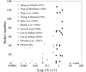
Figure 1 shows the available experimental data for solid–fluid flows published in Journal of Fluid Mechanics as a function of the Stokes number and the concentration (% v/v). For each reference, the dimensionless number was calculated using (1.1) from their respective reported conditions. Prominent studies for solid–fluid isotropic turbulence are not included in this figure as they operate in the absence of mean flow (Yang & Shy Reference Yang and Shy2005; Hwang & Eaton Reference Hwang and Eaton2006; Tanaka & Eaton Reference Tanaka and Eaton2010; Bellani et al. Reference Bellani, Byron, Collignon, Meyer and Variano2012). From figure 1 the lack of studies at concentrations higher than 0.8 % v/v for both intermediate and inertia-dominated regimes is apparent.

Figure 1. Experimental data previously published in Journal of Fluid Mechanics for solid–fluid flows. The  $x$-axis is the log of the solids concentration (% v/v) and the
  $y$-axis is the Stokes number.
In addition to the lack of information for concentrations above 0.8 % v/v, the majority of the two-phase flow experiments in the transition and inertia-dominated regimes used gas as the carrier fluid, with a few exceptions (Alajbegović et al. Reference Alajbegović, Assad, Bonetto and Lahey1994; Hosokawa & Tomiyama Reference Hosokawa and Tomiyama2004; Shokri et al. Reference Shokri, Ghaemi, Nobes and Sanders2017). Furthermore, as pointed out by Tanaka & Eaton (Reference Tanaka and Eaton2008), there is no information for Reynolds numbers above 30 000 aside from the recent work by Shokri et al. (Reference Shokri, Ghaemi, Nobes and Sanders2017) at a Reynolds number of 320 000. Finally, two-phase flow experimentation is so challenging that most of the studies report only the statistics for one of the phases, generally in the streamline direction. This scarceness of experimental two-phase flow data has been identified as a roadblock for the progress of computational models that need detailed information for validation and development (Fairweather & Hurn Reference Fairweather and Hurn2008; Balachandar & Eaton Reference Balachandar and Eaton2010).
The previous discussion indicates the need for liquid–solid experimentation in the intermediate and inertia-dominated regimes at Reynolds numbers above 30 000 and at concentrations higher than 0.7 % v/v. The present study aims to begin to fill this gap by providing information for solid–liquid turbulent flows at Reynolds numbers between 200 000 and 350 000 and concentrations from 0.7 % to 2.0 % v/v where no other data are available. The conditions for the experiments are presented in table 1. From the reported Stokes numbers, it can be noted that the flows range from the intermediate to the inertia-dominated regimes  $(St\geqslant 1)$. The non-intrusive optical techniques of laser Doppler velocimetry (LDV) and phase Doppler anemometry (PDA) are used to measure the velocity profiles. Although particle image velocimetry (PIV) is the most common method for the measurement of velocity, the LDV/PDA system was selected for its better temporal resolution, which is advantageous for flows having high-intensity fluctuations (Westerweel, Elsinga & Adrian Reference Westerweel, Elsinga and Adrian2013). Finally, the LDV/PDA point measurement is smaller than the standard PIV interrogation window, offering a better spatial resolution for the present application.
Table 1. List of variables measured at each of the experimental conditions:  $d_{p}$, particle diameter;
  $u$, axial mean and fluctuating velocity;
  $v$, radial mean and fluctuating velocity;
  $w$, theta mean and fluctuating velocity; and
  $\unicode[STIX]{x0394}P$, pressure drop. Subscript ‘
 $l$’ is for liquid and ‘
 $s$’ for solid. The Reynolds
  $(Re)$ and Stokes
  $(St)$ numbers are based on the pipe diameter and the bulk liquid axial velocity
  $(\boldsymbol{u}_{b})$ in the presence of the particles
  $(\boldsymbol{u}_{c}=1.2\boldsymbol{u}_{b})$, where
  $u_{c}$ is the liquid centreline velocity. For the particle Reynolds number
  $(Re_{p})$, the relative velocity at the centreline was used. A value of
  $1.002\times 10^{-6}~\text{m}^{2}~\text{s}^{-1}$ was used for the kinematic viscosity of water.

a Based on the equivalent volume sphere diameter.
b Crushed glass.
Besides the novelty of the conditions tested, the present dataset is comprehensive, consisting of: (i) direct measurement of the mean and fluctuating velocities for both the fluid and the solid phases in the axial, radial and tangential directions; (ii) pressure drops; (iii) concentration for each phase measured by direct sampling; (iv) profiles for the Reynolds stresses, the granular temperature and the kinetic energy; and (v) calculations for the turbulence modulation. The experiments were carried out in a vertical pipe test section in a pilot-scale facility using six different particle diameters, four concentrations, two densities, four different particle shapes and four Reynolds numbers. The flow configuration was upwards, which is ideal for the validation of computational models.
This paper is organized as follows. Next, § 2 presents a description of the experimental methods, including the pilot-scale experimental set-up, the LDV/PDA parameters and the procedure for the experimental runs. The limitations of the present experimental conditions are also discussed. Then § 3 presents the results, starting with the validation of the experimental set-up and the measuring techniques. The velocity profiles follow, showing the effects of particle size, concentration, Reynolds number, particle density and particle shape. Furthermore, the calculations of the Reynolds stresses and the turbulence modulation are presented, along with the measured pressure drops. Finally, § 4 presents the conclusions of the study.
2 Experimental methods
2.1 Materials
Water was used as the carrier fluid and solid particles as the dispersed phase for all the experiments. Microscope pictures of the particles used are seen in figure 2. Most of the experiments used spherical borosilicate glass particles (Dragonite Grinding Media, Jaygo Inc.) with a specific gravity (s.g.) of 2.55. Six sizes of spherical glass beads were tested, from 0.5 mm to 5 mm. Per manufacturer specifications, the particles were spherical with no surface cracks. According to the manufacturer, the 0.5 and 1 mm particles (type S) had a distribution from 0.5–0.75 mm and 1–1.30 mm, respectively. The particles in the range from 2–5 mm (type M) had a tolerance of 0.2 mm for the 2 mm beads and 0.3 mm for all other sizes. The crushed glass (Agsco) was crystal clear and had an s.g. between 2.45 and 2.55 per manufacturer specification. The crushed glass was sieved by hand to a final size distribution of  $2.8~\text{mm}<d_{p}<3.35~\text{mm}$, to be compared to the 3 mm spherical beads. Three types of steel particles were used, with the steel shot of 1 mm diameter (Erwin Industries, Amacast) having an s.g. of 10.9 and two sizes of stainless-steel cylinders (Norstone) with s.g. of 8.4 and dimensions of
  $1~\text{mm}\times 1~\text{mm}$ and
  $0.5~\text{mm}\times 4~\text{mm}$.

Figure 2. Pictures of the particles used in the present study: (a) 2 mm spherical beads; (b) 2 mm crushed glass; (c)  $1~\text{mm}\times 1~\text{mm}$ cylinders; (d)
  $0.5~\text{mm}\times 4~\text{mm}$ cylinders; and (e) 1 mm steel shot.

Figure 3. Diagram of the pilot-scale flow loop. Blue arrows indicate the flow direction,  $L$ is the vertical position in the pipe and
  $D$ is the pipe diameter. (1) Centrifugal pump, (2) venturi eductor, (3) electromagnetic flow meter (used during single-phase operation only), (4) developmental section, (5) pressure transducers separated five pipe diameters from each other, (6) test section, (7) three-way-valve bypass, (8) sampling tank (not present during the velocity measurements), (9) solids separation unit and (10) water tank. Inset: FEP test section showing the compensating box and the dual-beam LDV.
2.2 Experimental set-up
A pilot-scale set-up for the study of two-phase flows was designed by Pepple, Curtis & Yurteri (Reference Pepple, Curtis and Yurteri2010). The same set-up, albeit with a different test section, was used for the present experiments. The system, depicted in figure 3, allows for the study of vertical flow in an upward configuration. A centrifugal pump (Carver GH Series Pump, type  $4\times 3\times 10$ 20p impeller 8) was used to drive the flow from a water tank (900 gallon capacity) through a 78 mm (3 in.) schedule 40 type 304 stainless-steel pipe. The pump was controlled using a variable-frequency drive (ABB model number ACH550-UH-072A-4) (not shown in figure 3) that allowed the flow to be reproducible with an error less than 2 % at all speeds (Pepple Reference Pepple2010).
Particles entered the loop through a venturi eductor located at the bottom of a vertical stainless-steel pipe. Flow through the venturi created a reduction in pressure that pulled the particles into the flow. The particles could be stopped from entering the loop using a valve, which allowed the loop to operate in a single-phase or a two-phase configuration. The flow then entered the developmental section consisting of a segment of undisturbed path of 51 pipe diameters that allows the flow to become fully developed. The distance of 51 pipe diameters is well above the entrance length value of 16.6 required for a single-phase flow with  $Re=500\,000$ (the maximum Reynolds number used in the present study) according to the expression
  $L/D=0.623Re^{0.25}$ (Kays & Crawford Reference Kays and Crawford1980), where
  $L$ is the vertical position of the pipe and
  $D$ is the pipe diameter. The pressure drop was measured using four pressure transducers (Omega PX409C-015G5V-XL, linearity of 0.03 %) located at the end of the developmental section separated five pipe diameters from each other. The transducers gave three independent measurements of the pressure drop and were connected to a data acquisition unit (Omega OM-DAQ-USB-2401) with a 24-bit resolution.
The velocity profiles for the upward liquid–solid flow were measured in a circular test section using a two-component LDV/PDA set-up (TSI FSA3500/4000 and PDM1000). The curvature of circular pipes can create adverse conditions for optical techniques, including optical aberrations, reflections and modifications to the lenses’ focal points. In addition, changes in the refractive index from the test section to the fluid can exacerbate these problems. To prevent these optical complications, the test section was made from fluorinated ethylene propylene (FEP), which has a refractive index of 1.338, very close to that of water. The FEP pipe (Holscot Fluoroplastics Ltd, Grantham, UK) had an outside diameter of 80.52 mm (3.17 in.), an inside diameter of 77.22 mm (3.04 in.) and a length of 1 m. Furthermore, to circumvent the curvature issues, a compensating box filled with water was attached to the pipe, as shown in the inset in figure 3. The compensating box was specially machined to match the outside of the pipe (TMR Engineering) and had a borosilicate front glass with a thickness of 2.25 mm. The cell allowed an inner field of view of 114 mm and was glued to the FEP pipe with silicone. There was no back wall to the cell, so the glue was applied to the bottom and sidewalls only, allowing for the laser beams to enter through a flat boundary of glass into stagnant water. This configuration, modelled after the work from Brenn, Braeske & Durst (Reference Brenn, Braeske and Durst2002), resulted in no significant changes in the refractive index after the glass–water interface. It should be noted that there is a small difference of 0.8 mm between the stainless-steel pipe and the FEP test section. This small difference did not influence the stationary nature of the flow, as will be discussed in § 3. Pepple (Reference Pepple2010) also reported that the turbulence generated by differences in pipe diameters that were double the present value dissipated within a few pipe diameters.
After passing through the test section, the particles were removed from the water to prevent damage to the pump. The separation was done by gravity in the separation unit shown in figure 3. The particles, which were denser than the fluid, fell to the bottom of the vertical pipe where they were initially introduced, while water overflowed and went back to the water tank and subsequently to the pump. A mesh was placed in the top part of the solids separation unit to prevent particles from being carried into the water tank.
2.3 Velocity measurements with LDV/PDA and phase discrimination
LDV and PDA are common techniques in fluid mechanics and have been extensively used for two-phase flows as detailed in many studies (Albrecht et al. Reference Albrecht, Borys, Damaschke and Tropea2003; Balachandar & Eaton Reference Balachandar and Eaton2010; Tropea Reference Tropea2011). Briefly, the LDV technique measures the scattered light from particles at a specific point in the flow. The change in frequency of the scattered light is related to the velocity of the particles through the Doppler effect. In addition to the velocity, the PDA measures the size of the particles. In the dual-beam configuration, two laser beams are combined into a point called the measuring volume where dark and bright regions are created due to interference. These regions, called fringes, are used to measure the velocity component that is perpendicular to the fringes. If two velocities are of interest, two measuring volumes coincident in space, but perpendicular to each other, need to be used. In a two-component LDV, two different wavelengths are customary to discern the two velocity directions. For the present study, a green beam (514 nm) was used to measure the axial component, and a blue beam (488 nm) was used for the radial or theta components.
In a liquid–solid flow, the velocity measured by the LDV will be a combination of the scattered light from the tracer particles present in the fluid and the dispersed solid particles. A discrimination method is required to identify the velocity of each phase separately. This signal discrimination has presented a significant challenge in multiphase flow experimentation, with different techniques used to accomplish the separation. Some examples can be found in table 2.
Table 2. Phase discrimination techniques used in the study of two-phase flows.

Technique acronyms: LDV, laser Doppler velocimetry; PDA, phase Doppler anemometry; PIV, particle image velocimetry; PN, planar nephelometry.
Intensity discrimination is one of the methods most commonly used to measure individual phases (Tsuji & Morikawa Reference Tsuji and Morikawa1982; Tsuji et al. Reference Tsuji, Morikawa and Shiomi1984; Mychkovsky et al. Reference Mychkovsky, Rangarajan and Ceccio2012). Intensity discrimination is based on the principle that larger particles scatter a more intense light than smaller particles. Some studies rely on taking measurements using a particular photomultiplier setting targeted to a specific phase. For instance, a low gain in the photomultiplier can be used to mute the signal from small particles, which would allow for the measurements of the larger particles (Shuen, Solomon & Zhang Reference Shuen, Solomon, Zhang and Faeth1983; Kliafas & Holt Reference Kliafas and Holt1987). This approach has the disadvantage of being unable to measure the fluid phase in the presence of the particles due to cross-talk from the signals (Kliafas & Holt Reference Kliafas and Holt1987). The cross-talk can be produced by the trajectory ambiguity, the intrinsic distributions in size from the dispersed phase (not perfectly monodisperse) and the depth of field (Hardalupas et al. Reference Hardalupas, Taylor and Whitelaw1989; Albrecht et al. Reference Albrecht, Borys, Damaschke and Tropea2003). To avoid the interferences, some studies have used simultaneous channels tuned independently for each of the phases (Frishman et al. Reference Frishman, Hussainov, Kartushinsky and Rudi1999) or incorporate measurements of the Doppler amplitude (Tsuji & Morikawa Reference Tsuji and Morikawa1982). Some other studies combine different techniques as in Lau & Nathan (Reference Lau and Nathan2014), who used PIV along with planar nephelometry (PN). Another approach that has been successfully used for particles smaller than 1 mm has been to measure the velocity along with the size of the particles with the PDA (Gillandt et al. Reference Gillandt, Fritsching and Bauckhage2001; Kussin & Sommerfeld Reference Kussin and Sommerfeld2002). Having the size information allows for the signal originating from the tracers (usually having a size of only a few micrometres) to be separated from the larger dispersed phase. Finally, one of the most straightforward techniques is velocity discrimination, which can be used only when there is a significant slip between the particles and the flow (Alajbegović et al. Reference Alajbegović, Assad, Bonetto and Lahey1994).
For the present research, the PDA was used in conjunction with an intensity discrimination method to independently measure the liquid and the solid phases, respectively. As mentioned before, intensity discrimination is based on the fact that larger particles (the dispersed phase) scatter a more intense light than smaller tracer particles (continuous phase). The difference in signal intensity from each of the phases in the present study is presented in figure 4. The liquid velocity signal was originated by impurities present in tap water and had intensities below 500 mV when measured with the LDV in a backscatter configuration as observed in figure 4(a). The impurities in the water provided a sufficient source of velocity signal, and no further tracer particles were added. On the contrary, the intensity from the solid phase in the same optical configuration had higher values as seen in figure 4(b). Based on this difference, backscatter signals of more than 500 mV were classified as the solid-phase signal. In some cases, due to lower data rates, a smaller value of 400 mV was used as the limit for cases where the velocity separation was obvious. This lower value was selected only after observing the velocity versus intensity plots for each specific case and using a velocity discrimination step as additional validation.

Figure 4. Comparison of the LDV signal intensity for a flow at  $Re=200\,000$ as measured by the LDV in a backscattered configuration at the pipe centre for a (a) single-phase flow and a (b) two-phase flow with 4 mm particles at 2 % v/v. The dashed line at 500 mV marks the signal intensity level used for the phase discrimination of the solids.
The liquid velocity was not measured from the low-intensity signal to avoid the cross-talk effect. Instead, the PDA was used to measure the liquid by selecting only the signal from particles with a diameter below  $50~\unicode[STIX]{x03BC}\text{m}$. Different limits for the maximum diameter of the tracer particles were tested and showed no effect on the statistics (Mena Reference Mena2016). Particles with a diameter of
  $50~\unicode[STIX]{x03BC}\text{m}$ have Stokes numbers around 0.02, meaning that they belong to the macroviscous regime and follow the fluctuations of the fluid. The exception to the
  $50~\unicode[STIX]{x03BC}\text{m}$ limit were the data for the flow with 4 mm particles at a Reynolds number of 350 000 and a concentration of 2 % v/v. For this case, a stricter
  $20~\unicode[STIX]{x03BC}\text{m}$ limit for the maximum diameter was used because of particle attrition. Particle attrition only occurred after the flow loop had been running for several hours at the 2 % v/v concentration and the Reynolds number of 350 000, and was minimized by changing the particles and the water several times during the experiment. The fragmented pieces of glass were easily identified from the tracer as having a larger intensity and a lower velocity. These signals were successfully rejected with the
  $20~\unicode[STIX]{x03BC}\text{m}$ limit.
The reason for not using the PDA as the only discrimination technique is due to the large size of particles used in the present work (from 0.5 mm to 5 mm). Even by varying the collection angle, the maximum diameter that can be measured with the present PDA system is approximately  $750~\unicode[STIX]{x03BC}\text{m}$. Larger lenses for both the transmitter and the receiver units were tested, but signals were not found to be reliable.
Figure 5 shows the configuration for the measurements of the velocity data. The particle velocity was collected using the LDV in backscattering configuration, while the liquid velocity was collected using the PDA in forward scattering at a collection angle of  $30^{\circ }$. The transmitter is the same for both cases. These configurations provided the best quality of signal after testing different angles of collection. In addition, two different lenses were used in the transmitter probe for the measurement of the particle (focal length of 360 mm) and the liquid (focal length of 250 mm) velocities. The dimensions of the resulting measuring volume for each case are shown in table 3. The 250 mm lens allowed us to obtain the closest measurements to the wall but could not be used for the solid particles, as the probe volume was too small to get accurate readings.

Figure 5. Top view of the test section radius where each velocity component was measured. Also shown is the compensating box used to minimize changes in refractive index and curvature effects.
Table 3. Dimensions for the measuring volume in water for the different focal lenses on the current set-up. Here  $x$,
$x$,  $y$ and
  $z$ represent the Cartesian coordinates with the probe volume situated with its longest dimension along the
  $y$-axis.

Data were collected in coincidence mode, meaning that a measurement was only valid if the signals for both the green and blue measuring volumes were accepted by the processor using the acquisition parameters in table 4. The values for the acquisition parameters were optimized to give the best signal-to-noise ratio as judged by the burst efficiency, the data rate and the shape of the bursts as observed through an oscilloscope. The PDA signals had to meet two additional requirements to be accepted: (i) phase difference validation and (ii) intensity validation. The phase difference validation consists of comparing the two diameters that are independently measured for each burst using a three-detector configuration. If the difference between the two measurements is below 7 %, the signal is accepted (TSI 2005). The intensity validation procedure uses the curves for the theoretical prediction of the intensity of the scatter for different sizes. If the measured intensity falls between the predicted curves, the signal is accepted. This process is independent of the phase differences and allows for the rejection of erroneous signals from secondary scattering orders (TSI 2005; Mena Reference Mena2016). Finally, for the PDA, only the signal scattered from particles passing through the centre of the probe volume were collected by using a slit of  $150~\unicode[STIX]{x03BC}\text{m}$ that blocks all other regions of the probe volume.
Table 4. LDV and PDA parameters.

a For the single-phase runs with  $Re=500\,000$, the green beam was set to have a downmix of 36 MHz and a bandpass filter of 1–10 MHz.
b The ‘High’ signal-to-noise ratio setting on the TSI signal processor means that, for each Doppler burst to be valid, it must have at least seven valid cycles above the burst threshold limit (TSI 2005).
In the case of the LDV measurements, the photomultiplier tube (PMT) voltage was kept constant at all positions of the pipe to avoid changes in the signal intensity that would lead to erroneous phase discrimination readings (Hardalupas et al. Reference Hardalupas, Taylor and Whitelaw1989). For the PDA measurements, the PMT voltage and the burst threshold were varied as the probe volume traversed from the wall to the centre (lower PMT voltage at the wall, higher at the centre). The criterion for selecting the PMT for the PDA was to allow the data to follow the intensity validation curves.
In general, the burst efficiencies of the signals for both the LDV and the PDA were between 80 % and 100 %. For some measurements of radial components, the efficiencies in the secondary beam (blue beam) were lower than this value. The measurements were still judged acceptable, as they were taken in coincidence with the higher-efficiency signal from the primary beam (green beam) axial measurements.
2.4 Procedure for experimental runs
To ensure consistency in the selection of the different conditions, the first step for every run was to set the centreline velocity of the single-phase flow according to the Reynolds number to be studied (see appendix A). The velocity was measured using the LDV/PDA, and the pump frequency was adjusted as needed until the desired value was achieved. The electronic flow meter located before the developmental section was used at this point to corroborate the flow rate of the single phase. After the single-phase velocity was set, the solid particles were added to the system through the separation unit. The mass of particles added corresponded to a specific concentration as measured by direct sampling (see appendix A). After the two phases had equilibrated (10 min), a measurement at the centre of the pipe with the two-phase flow was collected. Data at this same location were taken at the end of the run (after  ${\sim}8{-}14~\text{h}$) to ensure the stationary nature of the measurements. For all experiments, these two measurements were found to be in agreement. The pressure drop was taken three or four times throughout the experiment. The data acquisition unit collected data at 250 Hz for approximately 10 min.
The axial and theta profiles were measured by traversing the probe volume from the wall to the centre of the pipe at specific steps and collecting the velocity data at each position. For the radial position, the probe volume was moved from the centre of the pipe to the wall (figure 5). To move the probe volume, the LDV/PDA optics were mounted in a three-dimensional Velmex Unislide traverse operated by a Velmex VP9000 controller. Approximately 20 radial positions were probed for the axial and theta components and 15 points for the radial component. Since the flow is axisymmetric, only measurements for half of the pipe were needed. At each position, a minimum of 400 points were taken to ensure the collection of a statistically significant number of data points as determined by a running average of the mean and standard deviation (figure 6). For the vast majority of the experiments, more than 500 points were collected at each radial position. Points that deviated from the mean by more than three times the standard deviation were considered outliers and were rejected (Compton & Eaton Reference Compton and Eaton1996). A new mean and standard deviation were calculated after the elimination of these points, and those are the values presented herein. In general, less than 2 % of the points were rejected from this procedure, as seen in table 5.

Figure 6. Example of a running average for the centreline axial velocity component of the liquid phase: (a) mean velocity and (b) fluctuating velocity. Data for flow with 5 mm particles at  $Re=200\,000$ and 0.7 % v/v. The mean of the velocity for 400 points is
  $3.05~\text{m}~\text{s}^{-1}$ with a standard deviation of
  $0.13~\text{m}~\text{s}^{-1}$. The dashed lines represent a 0.5 % variation for the mean and a 3 % variation for the standard deviation, which are within the 95 % confidence interval for the measurements. The data can be taken representing any of the conditions studied.
Table 5. Comparison of the number of points accepted for different limits of rejection. Here  $u$ is the mean velocity and
  $u^{\prime }$ the standard deviation. Data for a flow with 5 mm particles at 0.7 % v/v and
  $Re=200\,000$.

For all measurements, it was crucial to position the incoming laser beams perpendicular to the flat window in the test section. This alignment was accomplished using two square rulers. For the measurements of the axial and theta components, it was also important that the measurements were done from the wall to the centre of the pipe through the radius. To ensure the correct positioning of the transmitter, the laser reflections from the back wall were vertically aligned with the incoming beams. The exact location of the LDV/PDA probe volume inside the test section was calculated from a calibration relating the distance from the transmitter to the flat window in the test section. This calibration was done following the procedure by Durst, Muller & Jovanovic (Reference Durst, Muller and Jovanovic1988) and was confirmed by ray-tracing calculations (Mena Reference Mena2016). The distance was measured using a calliper (Mitutoyo Electronic Calliper, 0–60 in.).
After the measurement of the velocity profiles, the volumetric flow rate and solids concentration were measured by direct sampling. The flow was collected in a sampling tank (195 gallon Cylindrical Cone Bottom Tank from Chem Tainer Inc.) that was placed under the stainless-steel pipe (figure 3). A fast-release 4 in. gate valve (Atlantis Water Products, 400-Gate) was attached to the outlet of the tank and allowed the collection of the liquid and water mixture. The collection time was measured using a stopwatch. After the sample collection, the flow was diverted through the rubber pipe to avoid overflowing. The height of the solution collected was measured using a measuring tape, and the volume was calculated from geometry. The particles in the sampling tank were collected by opening the gate valve while keeping a mesh bag (MacMaster-Carr  $400~\unicode[STIX]{x03BC}\text{m}$ polyester mesh bag) in the outlet. The excess water from the particles was removed using a jet of high-pressure air before being weighed in a scale (Ohaus 110 lb Scale). The water content that remained in the particles is estimated to be less than 0.4 % of the weight after measuring the weight of the particles after they were totally dry.
2.5 Limitations on the experimental conditions
Table 1 shows the wide range of conditions studied. There are nine conditions for the glass beads where the three velocity components for each of the phases (solid and liquid) were measured, along with the pressure drop and the solids concentration. These are the base conditions in the present study, and they constitute a comprehensive dataset. Experiments at some conditions – like the different Reynolds numbers studied for the 4 mm particles – were specifically carried out to give more information on one particular velocity component, and measurements of the other components were not attempted. Additionally, there were some conditions where the measurement of the three velocity components was not possible due to low data rates. In these cases, data were collected for the velocity components that gave adequate data rates to provide as much information as experimentally possible. In general, signals for the liquid phase had higher data rates for lower volume fractions and larger particle diameters due to less scattering of the laser beams from the dispersed phase (the control parameter in the present study was the solids concentration, hence for the same level of concentration there are more particles present for smaller diameters). Conversely, for the solid phase, data from lower particle concentrations and higher particle sizes resulted in lower data rates since fewer particles would pass through the probe volume.
Additionally, the radial velocity component had lower data rates than the theta component, and the theta component had lower data rates than the axial component. Two phenomena caused this difference. (i) The green laser beam that is used to measure the axial component had a higher intensity than the blue beam used for the secondary components. The difference in intensity is a property of the beams exiting the beam splitter and results in higher data rates for the axial component. (ii) From figure 5, it can be noted that the laser beams travelled the entire pipe radius and the compensating box to reach the position where the radial component was measured. Along this path, there was absorption and scattering of the beams that lowered their intensity and consequently reduced the data rates.
Finally, since the solids concentration was measured by direct sampling, there were challenges due to splashing and difficulties diverting the higher flow rates through the three-way valve into the sampling tank. However, triplicates were conducted for one of the conditions and the sampling was performed at least once for each combination of Reynolds number, particle size and concentration. These direct measurements allowed for the estimation of the solids concentrations as a function of the Reynolds number and the mass of particles added to the flow. The measured volume fractions agreed with the data from Pepple (Reference Pepple2010) using the same set-up.
2.6 Uncertainty analysis
The variables measured in the present paper are the velocities of the particles and the liquid, the pressure drop in the pipe, the concentration of the particles and the location of the probe volume. For each variable, an uncertainty analysis was conducted that included the random and systematic sources of error as presented in table 6. To associate a level of 95 % confidence to the uncertainty, a coverage factor of 2 was used (Bell Reference Bell1999; Coleman & Steele Reference Coleman and Steele2009). Details of the calculations can be found in Mena (Reference Mena2016).
Table 6. Uncertainty of the measured variables expressed as a 95 % confidence interval.

a Calculated following the treatment by Yanta & Smith (Reference Yanta and Smith1973).
3 Results
3.1 Notation for the velocity profiles
The velocity profiles are presented using  $u$ as axial,
  $v$ as radial and
  $w$ as theta velocities. A subscript ‘
 $l$’ or ‘
 $s$’ designates the liquid (in the presence of the solids) or solid profile, respectively. The fluctuating component is denoted with a prime. For instance, the liquid axial fluctuations are
 $$\begin{eqnarray}\boldsymbol{u}_{l}^{\prime }=\sqrt{\frac{\displaystyle \mathop{\sum }_{i=1}^{N}(\boldsymbol{u}_{i,l}-\boldsymbol{u}_{\boldsymbol{l}})^{2}}{N-1}},\end{eqnarray}$$
 where  $\boldsymbol{u}_{i,l}$ is the instantaneous value of liquid axial velocity,
  $\boldsymbol{u}_{l}$ is the liquid axial mean velocity and
  $N$ is the number of data points collected (at least 400 for the present study).
The  $x$-axis in the velocity profiles represents the dimensionless radius, with 0 being at the centre of the pipe and 1 at the wall. The single-phase data are presented for comparison in all the two-phase plots using dashed lines. The single-phase data have been connected by a line intended to guide the eye. All velocities have been non-dimensionalized using the liquid centreline velocity in the presence of the particles. The plots include error bars representing a 95 % confidence interval (table 6). If the error bars are not visible, they are of the same size as or smaller than the marker symbols.
3.2 Validation of experimental set-up and measuring techniques
A series of validations tests were conducted to corroborate the accuracy of the experimental set-up and the data acquisition. They included the verification of the fully developed and axisymmetric nature of the flow, the successful reproduction of classical single-phase data, tests to determine the reproducibility of the experiments, and the verification that the wear of the particles was not influencing the measurements. The single-phase comparison to previous studies along with the corroboration that the flow is fully developed and axisymmetric are presented below. The rest of the validation records can be found in appendix B.
3.2.1 Reproduction of single-phase data
Single-phase measurements at a Reynolds number of 500 000 were conducted to compare the present measurements to the classical turbulent data by Laufer (Reference Laufer1954). The results for the mean and fluctuation velocities are shown in figure 7 and show that the present data follow closely the measurements reported by Laufer (Reference Laufer1954).

Figure 7. Single-phase velocity profiles for  $Re=500\,000$: (a) mean axial velocity and (b) fluctuating velocities in the axial, radial and theta directions. Open symbols are for the data from Laufer (Reference Laufer1954), while filled symbols are for the present data.
3.2.2 Fully developed flow
In a fully developed flow, the mean and fluctuation velocities do not change with axial position. To verify that the flow in the present set-up was fully developed, the velocity profiles in the presence of the particles were measured at two different axial locations in the test section as presented in figure 8 for a flow with 5 mm particles at a Reynolds number of 200 000 and a concentration of 1.2 % v/v. Location 1 was four pipe diameters (309 mm) downstream from location 2. There is an invariability of the velocity statistics at the two locations, showing that the flow is fully developed. An additional corroboration for this point comes from the pressure drop measurements for the same conditions presented in figure 8. Denoting  $D$ as the diameter of the pipe and
  $L$ as the vertical position in the pipe, where
  $L=0~\text{m}$ is at the bottom (see figure 3), the pressure drop between the bottom two pressure transducers at
  $L/D=31$ and
  $L/D=36$ was
  $10\,746.4~\text{Pa}~\text{m}^{-1}$. For the top two pressure transducers located at
  $L/D=41$ and
  $L/D=46$, the pressure drop was
  $10\,936.3~\text{Pa}~\text{m}^{-1}$. The difference between the two values is
  $190~\text{Pa}~\text{m}^{-1}$, which is within the uncertainty for the pressure drop measurements (table 6). If the flow were not fully developed, the pressure drop would decrease in the direction of the flow.

Figure 8. Solid velocity profiles measured at two different axial locations in the test section separated by four pipe diameters: (a) solid mean axial velocity and (b) solid axial fluctuations. Axial location 1 is downstream from axial location 2 (the flow is upwards). Flow with 5 mm particles at  $Re=200\,000$, and 1.2 % v/v.
3.2.3 Axisymmetry
The liquid velocity profiles for a flow with 1 mm particles were measured at two distinct radii, as shown in the inset in figure 9. The laser transmitter was located to the right of the position  $r2$. The measurements for
  $r2$ were taken at an off-axis angle of
  $150^{\circ }$ while those for
  $r1$ were taken at an off-axis angle of
  $30^{\circ }$. The velocity statistics for the two radii are in agreement with each other and show the symmetry of the flow. Measurements at other radii locations in the same set-up were also performed by Pepple (Reference Pepple2010) and further confirmed the axial symmetry.

Figure 9. Velocity profiles of the liquid phase for a flow with 1 mm particles at  $Re=200\,000$ and 0.7 % v/v: (a) liquid mean axial velocity and (b) liquid axial fluctuations. The inset circle represents the top view of the cross-section of the pipe and shows the location of the two radii represented by open and filled symbols, respectively. The laser source is to the right of
  $r2$.
$r2$.
3.3 Velocity profiles
As mentioned, the stationary nature of the flow was confirmed for every run by comparing the velocities from the first and last data point, which were collected at the centre of the pipe hours apart. Additionally, the integration of the solid velocity profile under the assumption that the solids were uniformly distributed was carried out to obtain the flow rate for the solid phase. The calculated flow rate was in agreement with the measured solid volume flow rate from the experiments. The data in tabular form are available as supplementary information available at https://doi.org/10.1017/jfm.2019.836.
The characteristic length of the most energetic eddies can be approximated by  $l_{e}\approx 0.2R$ (Hutchinson, Hewitt & Dukler Reference Hutchinson, Hewitt and Dukler1971), which is 7.7 mm for the present work. The other turbulence characteristic lengths for the single phase are presented in table 7 and show that the particles used are much larger than the Kolmogorov scale for all experiments and around the Taylor’s scale for the 0.5 mm and 1 mm particles. For the Taylor and Kolmogorov scales, the dissipation was estimated using the empirical relationship given by Afzal (Reference Afzal1982) as
 $$\begin{eqnarray}\unicode[STIX]{x1D716}=\frac{\boldsymbol{u}_{\unicode[STIX]{x1D70F}}^{3}}{R}\left(\frac{2.44}{\displaystyle \frac{y}{R}}-0.24\right),\end{eqnarray}$$
 where  $R$ is the radius of the pipe,
  $y$ is the distance from the wall and
  $\boldsymbol{u}_{\unicode[STIX]{x1D70F}}$ is the friction velocity, which can be estimated by the pressure drop according to Whitaker (Reference Whitaker1968) as
 $$\begin{eqnarray}\boldsymbol{u}_{\unicode[STIX]{x1D70F}}=\sqrt{\frac{\unicode[STIX]{x1D70F}_{o}}{\unicode[STIX]{x1D70C}}}=\sqrt{\frac{\displaystyle \left(\frac{\unicode[STIX]{x0394}P}{L}\right)_{frictional}\frac{R}{2}}{\unicode[STIX]{x1D70C}}},\end{eqnarray}$$
 where  $\unicode[STIX]{x1D70F}_{o}$ is the wall shear stress and
  $\unicode[STIX]{x1D70C}$ is the density of the fluid. It should be noted that the pressure drop in (3.3) corresponds to the frictional component of the pressure gradient.
Table 7. Taylor and Kolmogorov characteristic lengths of the single-phase data.

3.3.1 Effects of the particle size
Experiments using five sizes of particles with diameters from 0.5 mm to 5 mm were carried out at a Reynolds number of 200 000 and a concentration of 0.7 % v/v. According to the classification by Elghobashi (Reference Elghobashi1994), these flows belong to the dense suspension regime where both the particle–liquid turbulence interaction and the particle–particle collisions are important. The Stokes numbers for these tests ranged from 1 to 112 for the 0.5 mm and 5 mm particles, respectively, encompassing the transitional and inertia-dominated flows. For clarity, only the data from the 0.5 mm, 1 mm, 2 mm and 5 mm particles will be shown in this analysis. The profiles for the other diameters follow an intermediate behaviour according to their size.
The liquid mean axial velocity profile in the presence of the particles is shown in figure 10(a) and presents a maximum velocity at the centre of the pipe and a slight flattening with respect to the single phase. A flattening of the fluid profile was also observed in other studies in the transition and inertia-dominated regimes (Lee & Durst Reference Lee and Durst1982; Tsuji et al. Reference Tsuji, Morikawa and Shiomi1984; Hardalupas et al. Reference Hardalupas, Taylor and Whitelaw1989; Hadinoto et al. Reference Hadinoto, Jones, Yurteri and Curtis2005; Oliveira et al. Reference Oliveira, van der Geld and Kuerten2017). For the smallest particles used in the gas–solid flow experiments from Tsuji et al. (Reference Tsuji, Morikawa and Shiomi1984), there is a deviation of the maximum velocity from the pipe axis that is not observed in the present experiments.
The mean axial velocity profile for the different sizes of particles is presented in figure 10(b). The maximum velocity occurs at the centre, but it is much flatter than the liquid profile. Correspondingly, closer to the wall, the relative velocity becomes zero and changes sign. This change in sign can be explained by the fact that the particles engage in direct collision with the wall and do not lose all of their axial momentum upon collision. This phenomenon has been observed in other studies (Lee & Durst Reference Lee and Durst1982; Tsuji et al. Reference Tsuji, Morikawa and Shiomi1984; Alajbegović et al. Reference Alajbegović, Assad, Bonetto and Lahey1994; Kulick et al. Reference Kulick, Fessler and Eaton1994; Gillandt et al. Reference Gillandt, Fritsching and Bauckhage2001; Shokri et al. Reference Shokri, Ghaemi, Nobes and Sanders2017) and has been explained in the literature (Crowe et al. Reference Crowe, Sommerfeld and Tsuji1998). The position for the change in the sign of the relative velocity is roughly independent of particle size under the conditions studied.
In addition, figure 10(b) shows that the fluid–particle relative velocity increases with increasing particle size, which has been observed in other inertia-dominated flows (Tsuji et al. Reference Tsuji, Morikawa and Shiomi1984; Hardalupas et al. Reference Hardalupas, Taylor and Whitelaw1989; Sheen, Jou & Lee Reference Sheen, Jou and Lee1994; Lau & Nathan Reference Lau and Nathan2014; Shokri et al. Reference Shokri, Ghaemi, Nobes and Sanders2017). This increase in relative velocity can be explained by a decrease in particle drag with increasing particle size as described by the solid momentum balance for a steady-state flow:
 $$\begin{eqnarray}(\boldsymbol{u}_{l}-\boldsymbol{u}_{s})^{2}=\frac{4}{3}\frac{d_{p}(1-\unicode[STIX]{x1D6FC}_{s})^{1.65}[\unicode[STIX]{x1D6FC}_{s}\unicode[STIX]{x1D735}P+\unicode[STIX]{x1D735}P_{s}-\unicode[STIX]{x1D735}\unicode[STIX]{x1D749}_{s}-\unicode[STIX]{x1D6FC}_{s}\unicode[STIX]{x1D70C}_{s}\boldsymbol{g}]}{C_{D}\unicode[STIX]{x1D6FC}_{s}\unicode[STIX]{x1D70C}_{f}}.\end{eqnarray}$$
 Here subscript  $l$ is for the fluid and
  $s$ is for the solid,
  $\unicode[STIX]{x1D6FC}_{s}$ is the solid volume fraction,
  $P$ is the fluid pressure,
  $P_{s}$ is the solid-phase pressure,
  $\unicode[STIX]{x1D749}_{s}$ is the solid-phase stress tensor,
  $\unicode[STIX]{x1D70C}$ is the density and
  $C_{D}$ is the drag coefficient (Rowe Reference Rowe1961; Wen & Yu Reference Wen and Yu1966). It should be noted that the solid volume fraction is related to the solids concentration reported in the present paper by the relation
  $\%\,\text{v/v}=100^{\ast }\unicode[STIX]{x1D6FC}_{s}$.

Figure 10. Size effect on the mean axial velocity at  $Re=200\,000$ and 0.7 % v/v: (a) liquid and (b) solid.
The velocity fluctuations for the three components in the liquid phase are shown in figure 11. In general, the presence of particles flattens the liquid velocity fluctuations with augmentation in turbulence (relative to the single phase) observed in the core region of the pipe where the fluid–particle relative velocity is the highest. Specifically, in the core region, the larger 5 mm particles enhance the fluctuations for all three velocity components while the fluctuations from the smaller 0.5 mm and 1 mm particles increase less in the axial direction and are within the error bars of the single phase for the radial and theta components. The increase in fluctuations corresponds to an increase in particle Reynolds number from 1 to 2263 for the 0.5 mm and 5 mm particles, respectively, which leads to a turbulence enhancement from vortex shedding (Eaton & Longmire Reference Eaton, Longmire, Michaelides, Crowe and Schwarzkopf2017). Close to the wall, the particle size effect becomes negligible, and the fluctuations are within error bars from the single phase. Fluid fluctuations that increase with particle size have been found in other studies in the transition and inertia-dominated regimes (Lee & Durst Reference Lee and Durst1982; Tsuji et al. Reference Tsuji, Morikawa and Shiomi1984; Sheen et al. Reference Sheen, Jou and Lee1994; Kussin & Sommerfeld Reference Kussin and Sommerfeld2002; Hosokawa & Tomiyama Reference Hosokawa and Tomiyama2004; Hadinoto et al. Reference Hadinoto, Jones, Yurteri and Curtis2005; Shokri et al. Reference Shokri, Ghaemi, Nobes and Sanders2017). However, the  $70~\unicode[STIX]{x03BC}\text{m}$ data from Kulick et al. (Reference Kulick, Fessler and Eaton1994), at similar Stokes number to the present 2 mm particles but at a lower concentration of 0.02 % v/v, show attenuation of the turbulence.

Figure 11. Size effect on the liquid fluctuations at  $Re=200\,000$ and 0.7 % v/v: (a) axial component, (b) radial component and (c) theta component.
Figure 12 shows the effect of the particle size on the solid fluctuations. In general, the solid velocity fluctuation profile is much flatter than the fluid velocity fluctuation profile. For the solid axial fluctuations, the profile flattens with increasing particle size and the fluctuations increase with particle size at the pipe core. This increase in fluctuations is similar to that measured in the intermediate and inertia-dominated regimes by Hardalupas et al. (Reference Hardalupas, Taylor and Whitelaw1989) and (Shokri et al. Reference Shokri, Ghaemi, Nobes and Sanders2017), but it is in contrast to that encountered by Lau & Nathan (Reference Lau and Nathan2014) at the centre of the pipe. The data from Lau & Nathan (Reference Lau and Nathan2014) were collected at lower concentrations (0.04 % v/v) and Reynolds numbers (10 000–20 000) than the present results.
For the radial and theta fluctuations, their magnitudes are less than the single-phase fluctuations and decrease with increasing particle size. Lower solid radial fluctuating velocities were also measured in other works in the intermediate and inertia-dominated regime (Hardalupas et al. Reference Hardalupas, Taylor and Whitelaw1989; Alajbegović et al. Reference Alajbegović, Assad, Bonetto and Lahey1994; Kulick et al. Reference Kulick, Fessler and Eaton1994; Varaksin et al. Reference Varaksin, Polezhaev and Polyakov2000). However, Shokri et al. (Reference Shokri, Ghaemi, Nobes and Sanders2017) measured radial particle fluctuations that were higher than their single-phase fluctuations.
The flatness of the solid velocity fluctuation profiles is caused by a decrease in the shearing in the mean velocity field and the corresponding flat mean solid profile seen in figure 10(b). A flat solid fluctuating profile suggests a uniform solids concentration across the pipe, as indicated in dilute granular kinetic theory, which states that the solid volume fraction is inversely proportional to the granular temperature, where the granular temperature is proportional to the solid velocity fluctuations (Lun et al. Reference Lun, Savage, Jeffrey and Chepurniy1984). Basically, in regions where the particle velocity fluctuations are high, the mean free path associated with particle collisions is greater, corresponding to a smaller solids fraction.

Figure 12. Size effect on the solid fluctuations at  $Re=200\,000$ and 0.7 % v/v: (a) axial component, (b) radial component and (c) theta component.
Besides the base case study at Reynolds number 200 000, data at a Reynolds number of 350 000 were also collected. The difference between the liquid mean and fluctuating velocities due to particle size lessens as the fluid Reynolds number increases (data not shown). In fact, at the Reynolds number of 350 000, there is no observable effect from the particle size in the liquid and solid fluctuations for the conditions tested. Additionally, experiments with 1.2 % v/v at a Reynolds number of 200 000 were also conducted (data not shown). The same trends as with the concentration of 0.7 % v/v are observed except for the radial and theta fluctuations for the solid, where the larger particles have larger fluctuations than the smaller ones at the core of the pipe.
3.3.2 Effects of the solids concentration
Experiments with flows at four different concentrations ranging from 0.7 % to 2 % v/v were carried out at a Reynolds number of 200 000 using 4 mm particles. The Stokes number for these conditions was between 73 and 64, in the inertia-dominated region. For clarity, only the data for the highest and lowest concentration are presented, with the other concentrations having an intermediate behaviour.

Figure 13. Solids concentration effect on the mean axial velocity for a flow with 4 mm particles at  $Re=200\,000$: (a) liquid and (b) solid.

Figure 14. Concentration effect on liquid fluctuations for a flow with 4 mm particles at  $Re=200\,000$: (a) axial component, (b) radial component and (c) theta component.

Figure 15. Concentration effect on solid fluctuations for a flow with 4 mm particles at  $Re=200\,000$: (a) axial component, (b) radial component and (c) theta component.

Figure 16. Comparison of the effect of Reynolds number and concentration on the mean solid velocity for a flow with 4 mm particles: left-hand side,  $Re=200\,000$; right-hand side,
  $Re=350\,000$.
Figure 13(a) shows that increasing solids concentration flattens the mean liquid profile in the vicinity of the wall, as has been observed in other inertia-dominated flows (Tsuji et al. Reference Tsuji, Morikawa and Shiomi1984). Figure 13(b) shows that the relative velocity decreases with increasing concentration. Increasing solids fraction leads to an increase in the drag force on the particles, propelling the particle motion in the streamwise direction, as has been observed in other experiments (Tsuji et al. Reference Tsuji, Morikawa and Shiomi1984). However, Lee & Durst (Reference Lee and Durst1982) and Chemloul & Benmedjedi (Reference Chemloul and Benmedjedi2010) measured increasing relative velocities with increasing concentrations. The data from Chemloul & Benmedjedi (Reference Chemloul and Benmedjedi2010) were taken in a similar range of concentrations as the present data but at a lower Reynolds number of 16 200. The data from Lee & Durst (Reference Lee and Durst1982) were for lower concentrations and Reynolds number (0.06 % v/v and  $Re=8000$). These other trends hint at the influence of both the Reynolds number and the concentration on the relative velocity, which will be explored later in figures 16–20.
The liquid fluctuations for the three velocity components are shown in figure 14. The liquid axial fluctuations significantly increase with particle concentration, particularly at the core of the pipe, such that the resulting liquid fluctuating velocity profile is essentially flat. Increasing the number of particles increases the disturbance in the fluid due to increasing particle collisions and the resulting particle rotation associated with these collisions. The gas–solid experimental data from Tsuji et al. (Reference Tsuji, Morikawa and Shiomi1984), collected at concentrations below 0.6 % v/v in the inertia-dominated regime, also present an increase in liquid axial fluctuations with increasing concentrations. Hosokawa & Tomiyama (Reference Hosokawa and Tomiyama2004) also reported increasing liquid fluctuations with increasing particle concentration for their flows at 0.8 % v/v. The data from both Tsuji et al. (Reference Tsuji, Morikawa and Shiomi1984) and Hosokawa & Tomiyama (Reference Hosokawa and Tomiyama2004) were at lower Reynolds numbers than the data in figure 14 ( $Re=3.3\times 10^{4}$ and
  $Re=1.5\times 10^{4}$, respectively). The data from Hardalupas et al. (Reference Hardalupas, Taylor and Whitelaw1989), Kulick et al. (Reference Kulick, Fessler and Eaton1994) and Varaksin et al. (Reference Varaksin, Polezhaev and Polyakov2000) show a different trend at similar Stokes numbers, with decreasing axial fluid fluctuations at increasing concentrations, although their concentrations and Reynolds numbers were significantly lower (
 ${\sim}0.02$ % v/v,
  $Re=13\,000$;
  ${\sim}0.04$ % v/v,
  $Re=13\,800$; and
  $0.002$ % v/v,
  $Re=15\,300$, respectively). These different behaviours show that the Stokes number is only partly descriptive of the flow. In fact, it is remarkable how much the fluctuations change with increasing concentration in figure 14(a), although the four conditions have very similar Stokes numbers (see table 1).
Figure 14(b,c) presents the liquid fluctuations for the radial and theta components. It should be noted that the highest concentration that was possible for these measurements was 1.6 % v/v, as larger concentrations resulted in noisy signals. No significant effect of the particle concentration is observed for the radial or theta components at these conditions. A slight enhancement at the core is observed with respect to the single phase for both secondary components. All of the observed effects on the liquid velocity fluctuations with increasing particle concentration are more pronounced as the particle size increases (data not shown).
The solid fluctuations are presented in figure 15. The solid axial profile is very flat. The magnitude of the solid axial fluctuations is governed by (i) shearing in the mean phase (increasing fluctuations), (ii) increasing collisions with increasing concentration (decreasing fluctuations) and (iii) fluid fluctuations (enhancing or diminishing fluctuations). In the case of the results presented in figure 15, the observed enhancement of solid axial fluctuations with increasing solids concentration is likely to be due to (iii) the effect of the enhanced fluid fluctuations. Hardalupas et al. (Reference Hardalupas, Taylor and Whitelaw1989), Kulick et al. (Reference Kulick, Fessler and Eaton1994) and Chemloul & Benmedjedi (Reference Chemloul and Benmedjedi2010) measured solid fluctuating velocities that decreased with increasing concentration. Their experiments were performed at similar Stokes numbers but at much lower Reynolds numbers ( $Re=13\,000$, 13 800 and 16 200, respectively) and only the data from Chemloul & Benmedjedi (Reference Chemloul and Benmedjedi2010) were collected at similar concentrations. Figure 15(b,c) shows that the radial and theta components of the solids velocity fluctuations present no significant influence of the particle concentration at these conditions.
At higher Reynolds numbers, the profiles show a different trend with increasing concentration. Figure 16 shows the comparison between the mean solid profile for the Reynolds numbers of 200 000 and 350 000. As expected, an increase in Reynolds number decreases the relative velocity (see discussion in the next section dealing with the influence of the Reynolds number). However, it can be seen that the behaviour of the relative velocity with concentration changes: for the lower Reynolds number, the relative velocity decreases with concentration, whereas the opposite is observed for the higher Reynolds number. The behaviour of the relative velocity with concentration for the Reynolds number of 200 000 was explained due to an increase in drag force (see (3.4)). One possible explanation for the new trend at the Reynolds number of 350 000 involves the solid fluctuations behaviour shown in figure 17. For the Reynolds number of 350 000, the solid fluctuations decrease with increasing concentration, whereas the opposite occurs for the smaller Reynolds number. The reduction in solid axial fluctuations at the higher Reynolds number is caused by (i) a diminution in the source of particle fluctuations from the flatter mean profile observed in figure 16 and (ii) an increase in inelastic particle collisions at the highest concentrations. These solid fluctuations (granular temperature) influence the solid-phase pressure,  $P_{s}$, and the solid stress tensor,
  $\unicode[STIX]{x1D749}_{s}$, in (3.4). The solid-phase pressure includes the collision, kinetic and frictional components (
 $P_{s}=P_{s,col}+P_{s,kin}+P_{s,fr}$) (Johnson & Jackson Reference Johnson and Jackson1987). For the present study, there is no frictional component
  $(P_{s,fr})$ since the maximum solid volume fraction of 0.02 (2 % v/v) is below the value of 0.5 (50 % v/v) where enduring contacts are assumed to occur (LaMarche et al. Reference LaMarche, Morán, van Wachem and Curtis2017). The other two terms can be expressed as
 $$\begin{eqnarray}\displaystyle & \displaystyle P_{s,col}=2g_{0}\unicode[STIX]{x1D70C}_{s}\unicode[STIX]{x1D6FC}_{s}^{2}\unicode[STIX]{x1D703}(1+e), & \displaystyle\end{eqnarray}$$
 $$\begin{eqnarray}\displaystyle & \displaystyle P_{s,kin}=\unicode[STIX]{x1D70C}_{s}\unicode[STIX]{x1D6FC}_{s}\unicode[STIX]{x1D703}, & \displaystyle\end{eqnarray}$$
 where  $g_{0}$ is the radial distribution function,
  $\unicode[STIX]{x1D703}$ is the granular temperature and
  $e$ is the coefficient of restitution (Lun et al. Reference Lun, Savage, Jeffrey and Chepurniy1984). On the other hand, the solid stress tensor,
  $\unicode[STIX]{x1D749}_{s}$, is a function of the solid-phase viscosity
  $(\unicode[STIX]{x1D707}_{s})$ that can be represented as well by collision, kinetic and frictional components
  $(\unicode[STIX]{x1D707}_{s}=\unicode[STIX]{x1D707}_{s,col}+\unicode[STIX]{x1D707}_{s,kin}+\unicode[STIX]{x1D707}_{s,fr})$ (Johnson & Jackson Reference Johnson and Jackson1987). The collision and kinetic components are given by (Gidaspow Reference Gidaspow1994)
 $$\begin{eqnarray}\displaystyle & \displaystyle \unicode[STIX]{x1D707}_{s,col}=\frac{4}{5}\unicode[STIX]{x1D6FC}_{s}^{2}\unicode[STIX]{x1D70C}_{s}d_{p}g_{0}(1+e)\sqrt{\frac{\unicode[STIX]{x1D703}}{\unicode[STIX]{x03C0}}}, & \displaystyle\end{eqnarray}$$
 $$\begin{eqnarray}\displaystyle & \displaystyle \unicode[STIX]{x1D707}_{s,kin}=\frac{10\unicode[STIX]{x1D70C}_{s}d_{p}\sqrt{\unicode[STIX]{x1D703}\unicode[STIX]{x03C0}}}{96(1+e)g_{0}}\left[1+\frac{4}{5}g_{0}\unicode[STIX]{x1D6FC}_{s}(1+e)\right]^{2}. & \displaystyle\end{eqnarray}$$
The change in the trend of the solid fluctuations with concentration at the two Reynolds numbers in figure 17 along with (3.4) to (3.8) can explain the behaviour of the relative velocity in figure 16. At the lower Reynolds number, the increase in drag force with increasing concentration dominates, decreasing the relative velocity with increasing concentration. At the higher Reynolds number, the diminution in solid shear and the increase in particle collisions dominate, increasing the relative velocity with concentration. Such a complex relationship involving relative velocity, Reynolds number and concentration, as well as particle properties, has been well noted in the literature (Brucato, Grisafi & Montante Reference Brucato, Grisafi and Montante1998; Ghatage et al. Reference Ghatage, Sathe, Doroodchi, Joshi and Evans2013).
The comparison of the liquid axial fluctuations at the two Reynolds numbers is presented in figure 18. For the lower Reynolds number, the increase in the number of particles increases the disturbances in the flow, which in turn increase the liquid turbulence. But at higher Reynolds number the smaller relative velocity that creates less vortex shedding and the flatter mean solid profile result in less turbulence production and a smaller liquid fluctuation with increasing concentrations. The diminution of fluctuations with increasing concentrations observed in the axial component persists in the radial and theta components of the velocity fluctuations (figure 19).

Figure 17. Comparison of the effect of Reynolds number and concentration on the solid axial fluctuations for a flow with 4 mm particles: left-hand side,  $Re=200\,000$; right-hand side,
  $Re=350\,000$.

Figure 18. Comparison of the effect of Reynolds number and concentration on the liquid axial fluctuations for a flow with 4 mm particles: left-hand side,  $Re=200\,000$; right-hand side,
  $Re=350\,000$.
Higher concentrations also present a dampening effect in the solid and liquid fluctuations with increasing Reynolds number. Figure 20 shows the axial fluctuations for a flow with 4 mm particles at a concentration of 2 % v/v. As in figures 17 and 18, the fluctuations at the larger Reynolds number are not as flat as for the lower Reynolds number.

Figure 19. Profiles for the secondary velocity fluctuations for a flow with 4 mm particles at  $Re=350\,000$: (a) solid radial and (b) solid and liquid theta. The liquid velocities are represented by circles and the solid velocities by squares.

Figure 20. Effect of the Reynolds number on the axial fluctuations for a flow with 4 mm particles at 2 % v/v: (a) liquid and (b) solid.
3.3.3 Effects of the Reynolds number
Velocity profiles for two different Reynolds numbers of 200 000 and 350 000 were collected for a flow with 4 mm particles at a concentration of 0.7 % v/v. The flows are in the inertia-dominated regime having Stokes numbers of 73 and 125 according to their Reynolds number. Figure 21(a) presents the mean liquid axial velocity in the presence of the particles, showing a slight flattening of the profiles at the higher fluid Reynolds number. This trend is similar to that observed in single-phase flows with increasing Reynolds number. Figure 21(b) presents the mean solid axial velocity. The relative velocity decreases with increasing fluid Reynolds number, as the particles are more easily carried along with the fluid. Data from the transition and the inertia-dominated regimes at comparable concentrations to the present experiments also show a similar trend of diminishing relative velocity with increasing Reynolds numbers (Alajbegović et al. Reference Alajbegović, Assad, Bonetto and Lahey1994; Chemloul & Benmedjedi Reference Chemloul and Benmedjedi2010) – in the experiments from Alajbegović et al. (Reference Alajbegović, Assad, Bonetto and Lahey1994), the concentration was also changing along with the flow rate. The data from Hadinoto et al. (Reference Hadinoto, Jones, Yurteri and Curtis2005) at similar Stokes numbers, but at lower concentrations (0.03 % v/v), also show a smaller relative velocity with increasing Reynolds numbers.

Figure 21. Reynolds-number effect on the mean axial velocity for 4 mm particles and 0.7 % v/v: (a) liquid and (b) solid.

Figure 22. Reynolds-number effect on the liquid fluctuations for a flow with 4 mm particles at 0.7 % v/v: (a) axial component, (b) radial component and (c) theta component.
The liquid fluctuations at different Reynolds numbers are presented in figure 22. The axial fluctuating velocity is higher for the Reynolds number of 200 000. Since the relative velocity decreases with increasing Reynolds number, the particle Reynolds number also decreases from 1842 to 1126, and the augmentation of turbulence due to the wake effect is diminished. In contrast, at similar Stokes numbers, Hadinoto et al. (Reference Hadinoto, Jones, Yurteri and Curtis2005) showed an increase in the axial fluctuations for the fluid with increasing Reynolds numbers, while Alajbegović et al. (Reference Alajbegović, Assad, Bonetto and Lahey1994) did not observe much change in the liquid or solid fluctuations at the centreline. No influence of the Reynolds number is observed for the radial and theta liquid fluctuations under these conditions.

Figure 23. Reynolds-number effect on the solid fluctuations for a flow with 4 mm particles at 0.7 % v/v: (a) axial component, (b) radial component and (c) theta component.
The solid fluctuations are presented in figure 23. At the lower Reynolds number, the solid fluctuating velocity profile is flat, with the core region showing higher fluctuations than the single phase, corresponding to increased vortex shedding caused by higher relative velocities. As the Reynolds number increases, these solid fluctuations are dampened at the centre of the pipe. Lower fluctuations for the solid phase in the axial direction were also observed by Hadinoto et al. (Reference Hadinoto, Jones, Yurteri and Curtis2005). The data show that the solid fluctuations are smaller than the single phase. The theta solid fluctuating velocities are also lower than the single phase but do not show a marked effect on Reynolds numbers.
The reduction of liquid and solid fluctuations with increasing Reynolds number is also observed for higher concentrations (figure 20) and other particle sizes (data not shown).
3.3.4 Effects of the density of the particles
The effect of the density of the particles on the velocity profiles was studied by using glass (s.g. 2.5) particles and steel shot (s.g. 10.9) particles of 1 mm at a Reynolds number of 200 000. The solids concentrations were 0.7 % v/v and 0.1 % v/v for the glass and the steel, respectively. Figure 24 shows the mean axial velocities for the liquid and solid. As expected, the heaviest particles show a higher relative velocity. Larger relative velocities lead to higher vortex shedding, which results in larger axial fluctuations in both the liquid and the solid as seen in figure 25. Solid fluctuations that increased with increasing particle density were also observed by Kulick et al. (Reference Kulick, Fessler and Eaton1994). The liquid fluctuations in the secondary velocity components are not affected by the change in density under the conditions studied. The solid fluctuations of the steel particles present a slight diminution with respect to the glass particles, which was also observed by Kulick et al. (Reference Kulick, Fessler and Eaton1994).

Figure 24. Density effect on the mean axial velocity at  $Re=200\,000$ and 0.7 % v/v for the glass particles and 0.1 % v/v for the steel particles. The liquid velocities are represented by circles and the solid velocities by squares.

Figure 25. Density effect on the liquid and the solid fluctuations at  $Re=200\,000$ and 0.7 % v/v for the glass particles and 0.1 % v/v for the steel particles: (a) axial component, (b) radial component and (c) theta component. The liquid velocities are represented by circles and the solid velocities by squares.
3.3.5 Effects of the shape of the particles
Experiments with steel cylinders of different sizes were carried out at a Reynolds number of 200 000 and a solids concentration of 0.1 % v/v to study the shape effect on the velocity profiles. The two sizes of cylinders had a similar equivalent diameter as shown in table 8.
Table 8. Characteristics of the steel cylinders.

a  $Re_{p}$ uses the equivalent-volume sphere diameter.

Figure 26. Shape effect on the mean axial velocity at  $Re=200\,000$ and 0.1 % v/v. Filled markers represent the
  $1~\text{mm}\times 1~\text{mm}$ and open markers the
  $0.5~\text{mm}\times 4~\text{mm}$. The liquid velocities are represented by circles and the solid velocities by squares.

Figure 27. Shape effect on the liquid and the solid fluctuations at  $Re=200\,000$ and 0.1 % v/v: (a) axial component, (b) radial component and (c) theta component. Filled markers represent the
  $1~\text{mm}\times 1~\text{mm}$ and open markers the
  $0.5~\text{mm}\times 4~\text{mm}$. The liquid velocities are represented by circles and the solid velocities by squares.
Figures 24 and 26 show that the relative velocity for the  $0.5~\text{mm}\times 4~\text{mm}$ steel particles is slightly higher than for the
  $1~\text{mm}\times 1~\text{mm}$ steel particles, but both aspherical particles, due to their higher drag, have a reduced relative velocity compared to the 1 mm steel spheres. The small difference in relative velocity between the two aspherical particles could be due to differences in particle collision frequency. The higher-aspect-ratio particles will engage in more particle–particle collisions due to rotation. This increased collision frequency could give rise to some variations in local solids concentration over the radial cross-section, which in turn would influence the relative velocity.
While the liquid fluctuations and solid axial fluctuations are not significantly influenced by particle shape, figure 27 shows a profound influence on the solid fluctuations in the secondary components for the high-aspect-ratio  $0.5~\text{mm}\times 4~\text{mm}$ cylindrical particles. Figure 27(b,c) presents the only case in all the conditions studied where the solid fluctuations in the secondary components have a change in behaviour with respect to a variable that is not observed in the fluctuations in the streamwise direction. Figure 28 shows, via snapshots taken with a high-speed camera, that the high-aspect-ratio particles are not aligned with the flow. As noted before, these high-aspect-ratio particles will engage in increased particle–particle collisions, given that they are freely rotating and exhibit no preferential orientation. Guo et al. (Reference Guo, Wassgren, Hancock, Ketterhagen and Curtis2013) has shown via discrete element method simulations of granular flows of elongated cylinders that solid velocity fluctuations in non-streamwise directions are enhanced by particle rotation, but still lower than the streamwise velocity fluctuations. The experimental results shown here are consistent with these simulation results.

Figure 28. Still frames of the two-phase flow with steel particles at  $Re=200\,000$ and 0.1 % v/v: (a)
  $0.5~\text{mm}\times 4~\text{mm}$ cylinders and (b)
  $1~\text{mm}\times 1~\text{mm}$ cylinders.
Additionally, the shape effect was studied by comparing data for 3 mm glass spherical beads to crushed glass with a size distribution range between 2.83 mm and 3.28 mm at a Reynolds number of 200 000 and a concentration of 1.2 % v/v (data not shown). There is no effect of the particle shape on the velocity profiles under these conditions.
3.4 Reynolds stresses
The profiles for the Reynolds stresses, kinetic energy and granular temperature for a flow with 3 mm particles at a Reynolds number of 200 000 and a concentration of 1.2 % v/v are shown in figure 29. The Reynolds stresses for the liquid phase in the presence of the particles follow the behaviour of a single-phase flow (i.e. axial stress higher than theta, theta higher than radial). The kinetic energy of the liquid in the presence of the particles is higher than the single phase at the centre of the pipe. The granular temperature is roughly constant at all positions of the pipe.
Figure 30 shows the Reynolds stresses for the liquid and solid phases for different particle sizes at a Reynolds number of 200 000 and a concentration of 1.2 % v/v. The Stokes numbers are 40, 72 and 112 for the 3 mm, 4 mm and 5 mm, respectively. There is no observable effect of the particle size on the liquid Reynolds stresses at the conditions tested. The solid stresses increase with increasing particle size at the core of the pipe, but are indistinguishable from each other close to the wall.

Figure 29. (a) Reynolds stresses for the liquid in the presence of 3 mm particles at  $Re=200\,000$ and 1.2 % v/v. (b) Kinetic energy (circles) and granular temperature (squares) for a flow with 3 mm particles at
  $Re=200\,000$ and 1.2 % v/v. The Stokes number is 40.

Figure 30. Reynolds stresses  $\langle u^{\prime }v^{\prime }\rangle$ for (a) liquid phase and (b) solid phase for a flow with 3 mm, 4 mm and 5 mm particles at
  $Re=200\,000$ and 1.2 % v/v.
Figures 31 to 33 present the effect of the particle size, the concentration and the Reynolds number on the kinetic energy and the granular temperature. Figure 31(a) shows the kinetic energy for 3 and 5 mm particles at a Reynolds number of 200 000 and a concentration of 1.2 % v/v. Larger particle sizes increase the kinetic energy at the core of the pipe while there is no discerning effect closer to the wall. Figure 31(b) presents the granular temperature for the same conditions. There is no discernible effect of the particle size on the granular temperature under the conditions tested.

Figure 31. Size effect on (a) kinetic energy and (b) granular temperature at  $Re=200\,000$ and 1.2 % v/v.

Figure 32. Concentration effect on (a) kinetic energy and (b) granular temperature for a flow with 3 mm particles at  $Re=200\,000$.
Figure 32 presents the effect of the concentration on the kinetic energy (figure 32a) and the granular temperature (figure 32b) for a flow with 3 mm particles at a Reynolds number of 200 000. There is a slight increase in the kinetic energy at the centre of the pipe at higher concentrations. The granular energy decreases with increasing concentration. As the concentration increases, the number of inelastic collisions also increases, decreasing the solid fluctuations.
Figure 33 shows the effect of the Reynolds number on a flow with 3 mm particles and 0.7 % v/v. An increase in Reynolds number does not show a marked effect on the dimensionless kinetic energy or the granular temperature profiles for these conditions.

Figure 33. Reynolds-number effect on (a) kinetic energy and (b) granular temperature for a flow with 3 mm particles at 0.7 % v/v.
3.5 Turbulence modulation
The mechanisms of turbulence modulation are still not completely understood. There are many studies dealing with the topic, with excellent reviews available in the literature (Crowe et al. Reference Crowe, Sommerfeld and Tsuji1998; Balachandar & Eaton Reference Balachandar and Eaton2010; Eaton & Longmire Reference Eaton, Longmire, Michaelides, Crowe and Schwarzkopf2017; Subramaniam & Balachandar Reference Subramaniam, Balachandar, Basu, Agarwal and Mukhopadhyay2018). The magnitude and the sign of the turbulence modulation depend on the size of the dispersed phase, the Reynolds number and the concentration of the flow, among other variables. The many diverse parameters and their interplay make the analysis of turbulence modulation challenging. The early classification by Gore & Crowe (Reference Gore and Crowe1989) used the particle diameter  $(d_{p})$ divided by the fluid length scale of the most energetic eddies
  $(l_{e})$ as a delimitation parameter. In their work, they found that, when the ratio of
  $d_{p}/l_{e}$ is below 0.1, the presence of the second phase decreases the turbulence, whereas for ratios above 0.1 the second phase increases the turbulence. The value of 0.1 was thus defined as the critical ratio. A drawback with this definition is that the critical length-scale ratio does not take into account the concentration of the flow or the density of the particles (Tanaka & Eaton Reference Tanaka and Eaton2008). Another classification, proposed by Tanaka & Eaton (Reference Tanaka and Eaton2008), is the use of the particle momentum number
 $$\begin{eqnarray}Pa=St_{K}\,{Re_{L}}^{2}\left(\frac{\unicode[STIX]{x1D702}}{L}\right)^{3},\end{eqnarray}$$
 where  $St_{K}$ is the Stokes number based on the Kolmogorov scale,
  $\unicode[STIX]{x1D702}$ is the Kolmogorov scale,
  $L$ is the turbulence large length scale and
  $Re_{L}$ is the Reynolds numbers based on
  $L$. Two regions of turbulence augmentation were determined, separated by a region of attenuation between
  $Pa$ numbers of
  $10^{3}$ and
  $10^{5}$. It should be noted that, in solid–liquid flows, only augmentation has been reported (Tanaka & Eaton Reference Tanaka and Eaton2010). The present data will be evaluated using the critical ratio and the particle momentum number, although many other classifications exist (Michaelides Reference Michaelides2006).
Following the treatment by Gore & Crowe (Reference Gore and Crowe1989), the percentage change in turbulent intensity can be estimated by
 $$\begin{eqnarray}\%\text{ change in turbulent intensity}=\frac{\unicode[STIX]{x1D70E}_{TP}-\unicode[STIX]{x1D70E}_{F}}{\unicode[STIX]{x1D70E}_{F}}\times 100,\end{eqnarray}$$
 where  $\unicode[STIX]{x1D70E}_{F}$ and
  $\unicode[STIX]{x1D70E}_{TP}$ are the turbulent intensity for the single-phase fluid and the two-phase flow, respectively. The turbulent intensity for the single phase can be defined as (Whitaker Reference Whitaker1968)
 $$\begin{eqnarray}\unicode[STIX]{x1D70E}_{F}=\left(\frac{\sqrt{\overline{(\boldsymbol{u}^{\prime 2})_{single\;phase}}}}{(\boldsymbol{u}_{c})_{single\;phase}}\right),\end{eqnarray}$$
 where  $\boldsymbol{u}_{c}$ is the single-phase liquid centreline velocity, and
  $\boldsymbol{u}^{\prime }$ is the single-phase liquid fluctuating velocity. Similarly,
  $\unicode[STIX]{x1D70E}_{TP}$ is calculated with (3.11) using the values of the liquid centreline and fluctuating velocity in the two-phase flow configuration. Table 9 shows the values for the change in turbulent intensity for the different conditions studied in the present work.
Using the estimation by Hutchinson et al. (Reference Hutchinson, Hewitt and Dukler1971) for the integral scale  $l_{e}\approx 0.2R$, the particle diameter ratio to the fluid length scale for the present data results in 0.26 and 0.64 for the 2 mm and 5 mm particles, respectively. These values are above the 0.1 limit estimated by Gore & Crowe (Reference Gore and Crowe1989), meaning that the addition of the particles causes an increase in turbulence intensity. This is in agreement with the values calculated for the change in turbulence intensities seen in table 9, where all values are positive. In addition, the particle momentum number was calculated using a Stokes number
  $(St_{K})$ based on the Kolmogorov time scale for the fluid, the integral length scale as the large length scale
  $(L=l_{e})$ and the mean bulk velocity as the large velocity scale. The values for the particle momentum numbers are in the range
  $10^{3}<Pa<10^{5}$, which belong to what was classified as the attenuation region by Tanaka & Eaton (Reference Tanaka and Eaton2008). It should be noted that all other liquid–solid data analysed by Tanaka & Eaton (Reference Tanaka and Eaton2008) presented turbulence augmentation.
Table 9. Turbulence modulation for the different conditions for the glass beads. Here  $St_{K}$ is the Stokes number based on the Kolmogorov scale and
  $Pa$ is the particle momentum number.

a Particle Reynolds number calculated at the centre of the pipe.
Table 9 shows that, for the Reynolds number of 200 000, the solids concentration has a marked effect on the turbulent intensity, with higher concentrations presenting higher changes. Additionally, flows with larger particles have higher changes in the turbulent intensity than flows with smaller particles. However, higher velocities drown out these effects, with the data for 350 000 having smaller values of change in turbulent intensity irrespective of the particle size and the solids concentration. In fact, the experiments with Reynolds number of 350 000 presented the smallest changes in turbulence intensity. This trend was already observed in the velocity profiles at higher Reynolds number (see figures 18, 20, 22 and 23).
It can also be noted that higher turbulence enhancement should be expected with higher relative velocities due to vortex shedding (Hetsroni Reference Hetsroni1989). Nevertheless, the relative velocity does not hold a direct correlation with the turbulence enhancement, as some of the experiments with small relative velocity present large turbulence modulation (see the 2 mm particles at  $Re=200\,000$, for example). The Stokes number does not have a direct correlation with the turbulent modulation either, as was pointed out by Lucci, Ferrante & Elghobashi (Reference Lucci, Ferrante and Elghobashi2011) for particles larger than the Taylor microscale. In the present study, the particles with a diameter larger than 2 mm are larger than the Taylor microscale.
3.6 Pressure drop
The measured pressure drop in the vertical pipe is presented in figure 34(a) for varying glass particle sizes and in figure 34(b) for concentrations. The measured pressure includes the frictional and static components of the pressure. Three independent readings were obtained from the four transducers shown in figure 3. All readings were within error bars from each other. For clarity, only the results from one pair of transducers are shown in figure 34. The transducers used in figure 34 were separated by 763 mm (approximately 10 pipe diameters) as measured with a calliper. The error bars represent the expanded uncertainty to a 95 % confidence interval as estimated in the uncertainty analysis for the pressure drop and the velocity (table 6). As a reference, the predictions for the single-phase frictional pressure drop correlations from Kármán–Nikuradse and Petukhov (Kays & Crawford Reference Kays and Crawford1980) are included in figure 34 after the addition of the static pressure.
The pressure drop does not vary with the size of the particles for the conditions studied. However, the pressure drop increases with increasing concentration, with the increase being more significant at lower Reynolds numbers. An increase in pressure drop with solids concentration has been observed for micrometre-sized particles by Zisselmar & Molerus (Reference Zisselmar and Molerus1979) and Langsholt & Zarruk (Reference Langsholt and Zarruk2015) and for millimetre-sized particles by Tsuji et al. (Reference Tsuji, Morikawa and Shiomi1984), Ferre & Shook (Reference Ferre and Shook1998) and Matousek (Reference Matousek2009). In addition, Talmon (Reference Talmon2013) found an increase in friction factor with increasing concentration for 1.84 mm sand particles flowing in a vertical pipe at comparable velocities as the present conditions (less than  $5~\text{m}~\text{s}^{-1}$), although they found the opposite trend for the 0.37 mm particles. For particles smaller than
  $120~\unicode[STIX]{x03BC}\text{m}$ and concentrations less than 5 % v/v, Zisselmar & Molerus (Reference Zisselmar and Molerus1979) also found that the pressure drop of the mixture increased with concentration for all particle sizes.
A final point to be made from figure 34(b) is that the change in pressure drop with increasing concentration diminishes as the Reynolds number increases. This diminution in the effects of concentration with increasing Reynolds number was noticed in the velocity profiles presented in figures 16–18, and was also observed in the pressure measurements by Talmon (Reference Talmon2013).

Figure 34. Pressure drop (a) at 0.7 % v/v with different sizes of glass particles and (b) for a flow with 4 mm glass particles at different concentrations.
4 Conclusions
A comprehensive experimental dataset for turbulent solid–liquid flows in a vertical upward flow is presented for the intermediate and granular Stokes regimes for particle sizes from 0.5 to 5 mm, solid volume concentrations up to 2 % and Reynolds numbers from 200 000 to 350 000. These data start to fill a critical gap in knowledge regarding two-phase flow experimentation. The following general trends were observed.
For the conditions studied, the presence of the particles flattens the mean liquid profile close to the wall. At the pipe’s core, the velocity of the liquid in the presence of the particles does not deviate significantly from the single-phase values. The relative velocity has higher values closer to the centre of the pipe and decreases towards the wall, reaching a radial position where it changes sign. The radial position for the change in sign of the relative velocity is closer to the core for higher concentrations and higher Reynolds numbers and is roughly independent of particle size. Additionally, the relative velocity decreases with increasing Reynolds numbers.
The liquid axial fluctuating velocity is higher than the solid axial fluctuating velocity. The solid fluctuations present very flat profiles, with their values being below the single-phase behaviour at the wall. The axial velocity fluctuations for both the liquid and the solid decreased with increasing Reynolds number for the conditions tested.
Augmentation of turbulence is observed for all the conditions studied. The augmentation is in agreement with predictions by the critical ratio from Gore & Crowe (Reference Gore and Crowe1989) but in contrast to the particle momentum number by Tanaka & Eaton (Reference Tanaka and Eaton2008). In general, the turbulence intensity decreases with increasing Reynolds number and increases with increasing concentrations and particle sizes. Additionally, the pressure drop under the conditions studied is independent of the particle size and increases with increasing concentrations.
The Reynolds number is an influential parameter dictating the behaviour of the mean and fluctuating velocity profiles. For flows at a Reynolds number of 200 000, the relative velocity decreases with increasing concentration, whereas for flows at a Reynolds number of 350 000, the relative velocity increases with increasing concentration. The change in behaviour is also observed for the liquid axial fluctuations, which increase with increasing concentration at the smaller Reynolds number of 200 000 but decrease with increasing concentration at the higher Reynolds number of 350 000. This reversal in the trends with concentration shows the intricate coupling occurring between concentration, particle size and Reynolds number that influences the drag, the number of collisions, the shear and the fluctuations. In the present case, for the Reynolds number of 350 000, a decrease in the solid shear and an increase in the solid-phase pressure can explain the increase of the relative velocity with increasing concentration. For the lower Reynolds number of 200 000, an increase in the drag force with increasing concentration can explain the reduction in the relative velocity with increasing concentration.
Acknowledgements
The authors thank Professor K. Mohseni for the use of his high-speed camera and three-dimensional traverse. Funding from NSF OISE 0968313 is gratefully acknowledged.
Supplementary material
Supplementary material is available at https://doi.org/10.1017/jfm.2019.836.
Appendix A. Experimental conditions
The experimental conditions are summarized in tables 10 and 11.
Table 10. Single-phase centreline velocity selected at the beginning of each experiment.

Table 11. Mass of particles added for the different concentrations.


Figure 35. Data collected for a 2 mm slurry at  $Re=200\,000$ and 0.7 % v/v on three different days over a period of three weeks: (a) liquid-phase mean axial velocity, and (b) liquid-phase fluctuations.

Figure 36. Data collected for a 2 mm slurry at  $Re=200\,000$ and 0.7 % v/v on three different days over a period of three weeks: (a) solid-phase mean axial velocity, and (b) solid-phase fluctuations.
Appendix B. Validation of experimental data
B.1 Reproducibility of measurements
Repetitions of the measurements were carried for the 2 mm particles at  $Re=200\,000$ and 0.7 % v/v. These measurements were done weeks apart and are shown in figures 35 and 36. Liquid data are denoted by subscript ‘
 $l$’ while solid data are denoted by subscript ‘
 $s$’. From these graphs, it can be seen that the measurements are highly repeatable.
B.2 Effects of particle wear
To test if there was an effect of the wear of the particles on the velocity statistics, brand new 3 mm particles were tested against used particles for a flow at  $Re=350\,000$ and 0.7 % v/v. The results are shown in figure 37. No difference is observed between the data for the new and used particles.

Figure 37. Comparison of data obtained using new and used particles for a slurry with 3 mm particles at  $Re=350\,000$ and solid volume of 0.7 %: (a) liquid mean velocity, and (b) liquid fluctuating velocity. Circles denote used particles and squares denote new particles.


