


1. Introduction
Marine fisheries around the world are in a state of collapse to the extent that only about 20 per cent of stocks are moderately exploited or underexploited (FAO, 2009). The increased fishing pressure exerted by humans to meet the growing demand for food has led to overexploitation of marine resources. Nearly 1 billion people worldwide, or about 20 per cent of the global population, rely on fish as a primary source of animal protein. About 35 million people around the world are directly involved either part-time or full-time in fisheries primary production (UNEP, 2010a). The global fishing effort is 1.8–2.8 times larger than what the oceans can sustainably support (UNEP, 2010b). What this means is that humans are extracting more fish from the ocean than can be replaced by those remaining. The use of modern techniques to facilitate harvesting, transport and storage of fish has accelerated this trend. Modern fishing vessels cover large distances at high speed, from coastal zones to deep sea. They fish at great depths and stay at sea for several days, thus pushing fish populations below their sustainable limits.
Kerala, a leading maritime State in India, has been at the forefront of adopting innovative and new technologies in fishing practices.Footnote 1 The traditional fishing gears have been upgraded and newer, more efficient fishing techniques like trawls, seines, lines, gill-nets and entangling nets, and traps have been introduced. Some of the important technological changes that have taken place in the marine fisheries of Kerala are: the introduction of synthetic fishing gear materials, continuous improvement in the size, endurance, installed engine power, fish-holding and fuel capacities of the mechanized trawlers and gill-netters, adoption of modern technologies such as echo sounder and Global Positioning System (GPS) on a wider scale over the last decade, and the introduction of ring-seines with inboard engines in 1999 (Government of Kerala, 2010).
The growing demand for seafood and the adoption of modern fishing technologies have resulted in an intensification of fishing effort by both the mechanized and the motorized sectors, which in turn has put immense pressure on the marine resources. In the mechanized sector, time spent for fishing has increased through multiday, distant water fishing. In the motorized sector dimensional changes have been observed in the ring-seine gear which gives wider coverage and efficient catchability (Pillai et al., Reference Pillai2007). The length and breadth of the gear along with the capacity of the engines fitted to the boats have increased so as to provide quick mobility and faster access to the fishing grounds. All these changes have resulted in increased fishing efficiency causing concern for the sustenance of some of the exploited stocks.
Against the backdrop of the increase in fishing effort in the marine waters of Kerala, this study aims to investigate whether the actual level of catch and the corresponding fishing effort have exceeded the maximum levels necessary to support sustainable yield, or whether they are within the limits set by the maximum sustainable yield (MSY) levels. And to find that out, an aggregated Gordon–Schaefer model modified to include species diversity of the catch has been applied to marine fish catch and fishing effort data from Kerala for the period 1989–2004.
The paper is organized in six sections. Section 2 provides an overview of the marine fishing technology in Kerala. Section 3 sets out the modified Gordon–Schaefer model. While section 4 estimates the model, section 5 explains the data used. The final section uses the results to draw the conclusions.
2. An overview of the marine fishing technology in Kerala
Until the early 1950s, fishing technology in Kerala was predominantly artisanal or traditional. It was marked by the use of oars or sails for propulsion, selective and passive gears with low capital investments, and the use of traditional knowledge and fishing skills mainly for subsistence purposes. However, with the arrival of the Indo-Norwegian Project in 1953, another sector popularly known as the ‘mechanized sector’ consisting of trawlers, gill-netters, and purse-seiners emerged and gained strength (Paul, Reference Paul2005).
The mechanized sector and the traditional sector were the only two sectors involved in the exploitation of marine fisheries until the 1980s. During the early-mid 1980s, traditional crafts were rapidly motorized with outboard motors for propulsion. This was in response to the difficulties faced by the traditional fishermen due to the operation of mechanized trawlers and purse-seiners. Penaied prawn, a demersal fish variety and the most-valued export item of the State, was fished by mechanized trawlers that indiscriminately dragged and disturbed the entire sea bottom, thereby destroying eggs and larvae of different varieties of fish in the inshore sea bottom. The new motorized crafts became an integral part of the indigenous fisheries and the fishers could extend their activities to more distant and deeper waters using these crafts. In the latter half of the 1980s, a new gear called ring-seine became very popular in exploiting the pelagic resources, and replaced the boat-seines to a very large extent. Thus a new sector called the ‘motorized sector’ developed within the traditional sector. Hence today, there are three sectors operating in the marine waters of Kerala viz., motorized traditional, nonmotorized traditional and purely mechanized.
Trawlers are most commonly used in the mechanized sector, followed by gill-netters, purse-seiners, and long-liners, whereas in the motorized traditional sector ring seines are more popular. In the nonmotorized traditional sector, gill-nets, long-lines, and shore-seines are commonly used.
Table 1 provides a detailed account of the changes in landings and fishing effort using different fishing techniques in Kerala's marine fishery. Mechanized trawl-nets accounted for the highest share in the total fish landings in 1989–1993 at around 39 per cent, but in 2000–2004, landings by trawl-nets were a percentage lower (with a share of 36 per cent in the total fish landings) than those by the motorized ring-seines. In absolute terms, the total fish landings using trawl-nets declined from 1,181 thousand tonnes in 1989–1993 to 1,060 thousand tonnes in 2000–2004. Though the share of motorized ring-seines remained more or less the same at around 37 per cent in both the periods, in absolute terms the landings declined from 1,111 thousand tonnes in 1989–1993 to 1,083 thousand tonnes in 2000–2004. Also, mechanized ring-seines, which were not seen earlier, contributed around 4 per cent to the total landings in 2000–2004.
Table 1. Changes in fish landings and fishing effort from 1989–1993 to 2000–2004 (percentage contribution to total change in fish landings by different fishing techniques is also shown)
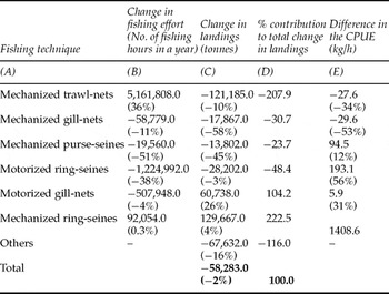
Note: Figures in parentheses in column (B) represent the percentage change in the fishing effort from 1989–1993 to 2000–2004 while in column (C) they represent percentage change in the annual fish landings from 1989–1993 to 2000–2004. In column (E), figures in parentheses represent the change in the CPUE from 1989–1993 to 2000–2004.
Source: Computations by the author using landings and effort data taken from the Central Marine Fisheries Research Institute, Kochi.
The fishing effort measured in terms of the annual fishing hours increased for mechanized trawl-nets and mechanized ring-seines from 1989–1993 to 2000–2004, but for other fishing techniques there was no corresponding increase during the same period. Fish landings, on the other hand, increased only in the case of motorized gill-nets by about 26 per cent. The decrease in fish landings in the case of mechanized trawl-nets was around 10 per cent, whereas in the case of mechanized gill-nets it was around 58 per cent. As for mechanized purse-seines it was 45 per cent, and for motorized ring-seines it was 3 per cent. The overall decline in fish landings was around 2 per cent during the same period. An important contributor to this decline was the fall in fish landings using mechanized trawl-nets (around 208 per cent). Other techniques like mechanized gill-nets, purse-seines, and motorized ring-seines together contributed around 103 per cent to the total decline in fish landings. A decline in the total fish landings of the order of 117 per cent was due to the fall in the landings using other fishing techniques. Finally, motorized gill-nets and mechanized ring-seines together increased the total fish landings by about 327 per cent.
A comparison of the landings, the effort and the catch per unit effort (CPUE) across different fishing techniques provides some interesting insights. Rising fishing effort, and falling landings and CPUE in the case of mechanized trawl-nets suggest that there is a possibility of stocks fished using trawl-nets getting depleted. As a result, it is quite likely that the trawler operations are facing negative returns. On the contrary, the changes in fishing effort and landings using motorized gill-nets suggest that the catching efficiency of this technique has improved, though it is not clear as to why it is so. For fishing operations using mechanized gill-nets, the fall in the landings is far more than the fall in the effort, meaning thereby that the landings are quite sensitive to the fishing effort. In other words, this fishing technique appears to be quite efficient in fish catch.
The CPUE compared to the above has increased for mechanized purse-seines and motorized ring-seines even with falling fishing effort and fish landings. The fall in the fishing effort is more than the fall in the fish landings, especially in the case of motorized ring-seines. It is possible that motorized ring-seine operations are experiencing diminishing returns. In such a case fishing effort can be lowered substantially without a significant decrease in fish landings. Finally, the changes in landings and effort cannot be observed for mechanized ring-seines since only recent landings and effort data are available for this fishing operation.
In conclusion, there are some fishing techniques with diminishing or negative returns while the catching efficiency of others has increased. And for some techniques it is difficult to explain the changes in landings and effort over time. Looking at the figures alone it is difficult to point out the direction in which the overall landings and fishing effort are moving; have they crossed the sustainable yield level or are they below it?
In the next section, I aim to address this issue by estimating the limits to sustainable fish catch and fishing effort, using the modified Gordon–Schaefer model, and comparing these limits with the actual average values of fish catch and fishing effort.
3. The modified Gordon–Schaefer model
This section sets up the modified Gordon–Schaefer model for fish-catch from the marine waters of Kerala.Footnote 2 A biological model of multispecies fishery is generally complex for the present study because of the nature of the data required.
The Gordon–Schaefer model is a surplus production model. It has the big advantage of requiring limited data only, but along with this a simplifying assumption in the model has to be made. The Gordon–Schaefer model is a single-species model and therefore, by necessity, its application to a multispecies and multigear fishery produces only a rough guidance on the desirable fishing effort (Kasulo and Perrings, Reference Kasulo and Perrings2006).
It is postulated initially that the catch is determined by the effort involved in extraction, and the stock of fish, i.e.,
where Y is the catch rate or harvest rate, E is the effort involved in extraction and X is the fish stock.
The Gordon–Schaefer model assumes a logistic growth function for fish biomass (stock), and a simple Cobb–Douglas production function for fish catch Y as a function of fishing effort E and fish stock X. It can, therefore, be written as
where r is the intrinsic growth rate of fish stock and K is the maximum environmental carrying capacity.
The Gordon–Schaefer fish production function,
assumes that the catch rate is directly proportional to the effort rate E and to the available biomass X, while q is the catchability coefficient.
The change in stock biomass in a given time period is expressed as the difference between the natural growth and the harvest. Suppressing time subscripts the change in biomass can be expressed as
At the steady state, ![]() and the Gordon–Schaefer fish production function Y can be written as
and the Gordon–Schaefer fish production function Y can be written as
The modification to the Gordon–Schaefer model includes the effect of the species diversity of the harvest on the growth of the fish stocks. The study of biodiversity includes ecological and economic considerations. The ecological aspect relates to human actions that affect the number and the persistence of species, while the economic aspect looks at the economic driving forces that affect biodiversity as a result of human intervention, and are a cause of their loss (Gupta and Bhattacharya, Reference Gupta, Bhattacharya, Kumar and Reddy2007). The economic value of biodiversity is important because it determines the level of both its use and its conservation. A pattern of ‘sequential exploitation’ of fish resources occurs from accessible to less accessible areas and from valuable to less valuable species. The reason behind such an occurrence is that fisheries are market driven and thus a higher fishing effort is directed towards species which are more economically valuable than the others. Kasulo and Perrings (Reference Kasulo and Perrings2006) have called this phenomenon ‘fishing down the value chain’.
In this study, biodiversity is measured by an index of the species diversity of the catch. Two indices are used: an unweighted and a price-weighted Simpson's index.Footnote 3 Simpson's index is a simple mathematical measure that characterizes species diversity in a community. The proportion of species i relative to the total number of species is calculated and squared, i.e., ![]() where Yit is the catch of the ith species harvested in period t, Yt is the total catch in period t, and st is the number of species harvested in period t; is a measure of species dominance. The price-weighted Simpson's index, on the other hand, is defined as
where Yit is the catch of the ith species harvested in period t, Yt is the total catch in period t, and st is the number of species harvested in period t; is a measure of species dominance. The price-weighted Simpson's index, on the other hand, is defined as ![]() , where
, where ![]() is the market value of the total fish catch and Pi is the unit price of species i.
is the market value of the total fish catch and Pi is the unit price of species i.
The value of B*t is determined by the changes in the market conditions for different species and the changes in the species composition over time due to natural causes and fishing pressure. The value of both the indices, price-weighted and unweighted, ranges between 0 (infinite diversity) and 1 (no diversity). The higher the value of the index, the lower is the sample diversity. When all the species caught have the same market value, then the solution for the weighted index is the same as for the unweighted index. If different species have different market values, the impact of price weighting depends on the relative abundance of the more- and the less-valued species. When the community is dominated by species of high (low) market value, the economic biodiversity index will be greater (lesser) than the corresponding ecological biodiversity index.
In the Gordon–Schaefer model, the effect of species diversity on fish productivity is captured by the introduction of an additional term in the fisheries production function,
where B is the biodiversity index and BE is the biodiversity adjusted effort applied to fishery. Put differently,
When biodiversity-adjusted effort is introduced in the standard model, the following growth function is obtained:
and in the steady-state equilibrium, the sustainable yield function becomes:
4. Reduced form of equations and estimation of parameters
In order to estimate the parameters of the model, the Schnute (Reference Schnute1977) method is used. Under this estimation method, Schaefer's production model is reduced to a form making it amenable to annual data on catch and effort.
An equation for CPUE can be defined in terms of U, with and without the biodiversity index. Without the biodiversity index, given Y = qEX, and ![]() , or U(t) = qX(t), where CPUE U(t) is proportional to biomass alone.
, or U(t) = qX(t), where CPUE U(t) is proportional to biomass alone.
The growth equation (1) expressed in terms of U can be written as
Similarly, with the biodiversity index B the growth function as given in equation (2) can be rewritten in terms of U as
Equations (1a) and (2a) can now be used to obtain the reduced form. By adding time subscripts and integrating from t − 1 to t, equations (1a) and (2a) can be expressed as
with U being defined with and without the biodiversity index as Ut and Ubt, respectively.
A linear regression of ![]() against the two variables, Et and Ut, is used to estimate the parameters r, q, and K. In the end, the following three equations are estimated:
against the two variables, Et and Ut, is used to estimate the parameters r, q, and K. In the end, the following three equations are estimated:
Here,
Ut is the CPUE, and the annual level of fish biodiversity of the catch is measured by Bt. The dependent variable is an index of relative change in fish biomass.
5. Description of the model variables
For model estimation, data are needed on annual marine fish landings, effort involved in marine fish catch (a proxy variable for the entire input bundle is used), diversity indices (biological and bioeconomic) and the ratio of fish catch to effort involved in fish catch.
Catch Yt is the marine fish landings in Kerala from 1989 to 2004, measured in thousand tonnes. The marine fish landings in Kerala mainly consist of Perches, Carangids, Clupeids, Mackerels, Pomfrets, Threadfins, Croakers, Flatfishes, Ribbonfishes, Molluscs, and Crustaceans. These can be divided into two groups, pelagic and demersal. Some of the important pelagic species are Oil Sardines, Indian Mackerel, Scads and Ribbonfishes, and the important demersal species are Penaeid prawns, Threadfin breams, Cephalopods, and Croakers. The landings of both pelagic and demersal fish show an average annual decline of 0.5 and 1.3 per cent, respectively from 1989 to 2004. The decline in pelagic fish is from 434.85 thousand tonnes in 1989–413.65 thousand tonnes in 2004, while the decline in demersal fish is from 212.53 thousand tonnes in 1989 to 203.18 thousand tonnes in 2004. The average annual rate of decline in the overall landings is around 0.2 per cent for the same period. Figure 1 depicts the trend in marine fish landings (total, pelagic and demersal) in Kerala from 1989 to 2004. The data on fish landings are taken from the Central Marine Fisheries Research Institute (CMFRI), Kochi.

Figure 1. Marine fish landings in Kerala - total, pelagic and demersal, 1989–2004.
Standardized effort, Et – data on two different measures of fishing effort are taken from the CMFRI, viz., the actual number of fishing hours spent in a year using each fishing technique, and the corresponding number of fishing trips made in a year. For the purpose of analysis, effort units for each technique are converted into a single standardized effort unit (thousand fishing hours using purse-seines in a year).Footnote 4 The standardized effort unit is calculated by multiplying the total number of fishing hours spent in a year by each fishing technique (ei) by a standardizing weight (wi) summed over all the fishing techniques (i), that is, Et = ∑i wi × ei. The weight used is the average yearly catch per trip using each technique divided by the average yearly catch per trip using purse-seines. The resulting fraction is used to convert different techniques into purse-seine hours.Footnote 5 The specific weights are shown in table 2.
Table 2. Weights assigned to different fishing techniques

Source: Computations by the author using fishing effort data taken from the Central Marine Fisheries Research Institute, Kochi.
An increasing trend is observed in the standardized effort applied to fish catch (figure 2). The standardized effort has increased at an average annual rate of almost 1.3 per cent.

Figure 2. Standardized effort applied to marine fish catch in Kerala, 1989–2004.
Effort adjusted for biodiversity is defined as EtBt. This is further adjusted for bioeconomic diversity, defined as EtB*t. Since the diversity indices are fractions, the units for Et, EtBt, and EtB*t are the same.
Catch per unit effort Ut is obtained by dividing the total annual fish catch by the annual standardized effort applied to fish catch. CPUE is measured in kg/unit std. effort. Figure 3 shows the declining trend in CPUE. The average annual rate of decline is 1.2 per cent.

Figure 3. The total catch per unit of standardized effort for marine fish catch in Kerala, 1989–2004.
Like effort, CPUE is also adjusted for both biological and bioeconomic diversity. CPUE adjusted for biological diversity is given by UtBt and by UtB*t for bioeconomic diversity.
The value of the unweighted Bt and price-weighted B*t biodiversity indices constructed using Simpson's index for the fishery are shown in figure 4.

Figure 4. Biodiversity and bioeconomic indices for marine fish catch in Kerala, 1989–2004.
The value of the unweighted index is falling until 1998, indicating that the diversity of catch i is rising. The price-weighted index, on the other hand, is generally higher than the unweighted index – and sometimes quite higher, suggesting that the fishers are focusing on high-valued species. From the year 1999, the price-weighted index begins to fall, indicating that the catch is dominated by low-valued species, whereas the value of the unweighted index begins to rise, indicating that diversity of catch is falling.
During the period 1989–1998 the fishery was dominated by the high-valued penaeid prawns and to some extent by Stomatopods and Cephalopods, emphasis was also on low-valued Oil Sardines and Indian Mackerel. In the period 1999–2004, high-valued penaeid prawns continued to dominate the fishery along with low-valued Oil Sardines, Indian Mackerel and Ribbonfishes. Oil Sardines accounted for the highest share in the total quantity of fish catch, while penaeid prawns dominated in terms of value of fish catch.
Last of all,Xt, the dependent variable for the model, is constructed by taking the ratio of the current over the lagged values of Ut, UBt, and UB*t.
6. Results and discussion
Regression results for equations (3a), (4a), and (4b), corrected for autocorrelation using a Prais-Winsten transformation, are reported in table 3. A residual test to check for serial correlation is also conducted.Footnote 6
Table 3. Regression results after correcting for autocorrelation

Note: t-statistics given in parentheses.
For equation (1), all the parameter estimates are statistically significant and the model explains 65 per cent of the variation in fish biomass. The corresponding F-statistic is also statistically significant. Addition of the unweighted biodiversity index (equation (2)) improves the goodness of fit. The parameter estimates are statistically significant and the model explains 66 per cent of the variation in fish biomass. Introduction of price-weighted bioeconomic diversity index in the final equation (3) further improves the goodness of fit. The model now explains 71 per cent of the variation in fish biomass.
The model reports that it is possible to explain a high proportion of the variation in fish biomass if the model includes a measure of the diversity of catch. The parameter estimates from equation (3), along with the average value of the price-weighted biodiversity index, are used to calculate the MSY levels of fish catch and effort.Footnote 7 The MSY levels of catch and effort are sensitive to changes in the level of biodiversity and to changes in the value of the estimated parameters. Before proceeding with the results of equation (3), a Wu-Hausman test is conducted to test the null hypothesis of exogeneity of the input variable, fishing effort. The test results confirm that the fishing effort is exogeneously determined.Footnote 8 The actual and MSY levels of catch and effort with their respective t-statistic values are presented in table 4.
Table 4. MSY and actual levels of catch and effort
Note: t-statistics given in parentheses.
The estimated MSY level of effort is statistically significant at 1 per cent whereas the MSY level of catch is statistically insignificant. The MSY solution for fish catch is finally dropped due to insignificant t-statistic value. For comparison purposes only effort figures are used. The average fishing effort applied from 1989 to 2004 is more than what the maximum effort should be in order to achieve sustainable fish yield. What impact this increased fishing effort has on fish catch cannot be stated since the MSY catch level is not known.
In sum, it is evident from the model results that actual fishing effort has exceeded the level necessary to maintain sustainable fish yield. In addition, table 1 clearly shows that the fishing effort exerted by some techniques is more than the gains in terms of the quantity of fish catch, meaning that there is a potential to decrease the current level of fishing effort without undergoing a significant decline in fish catch. However, the extent of decline in the fishing effort and the sustainable catch limit has to be decided for each technique separately. The present model only estimates the MSY levels of catch and fishing effort applied by all the techniques put together. A similar model can be constructed to estimate the MSY levels of catch and effort for each fishing technique. Given the paucity of data, such an analysis cannot be undertaken in the present study. Nevertheless, the usefulness of this analysis lies in defining the desirable fishing effort, taking into account the existing species diversity in the current scenario.
7. Limitations of the study
An important limitation of the study is the nonavailability of fishing effort data for a longer period, though the fish landings data are available. The analysis is carried out using data for only 16 years. Another important limitation is the lack of availability of reliable data on cost of effort, failing which the model could not be run for open access and profit maximization regimes. As a final point, in the present model a measure of environmental conditions could not be included due to lack of robust studies on the relationship between environmental conditions and fish biomass in the marine waters of Kerala.
Appendix A: Catch per unit effort using different fishing techniques for marine fish catch in Kerala
Figure A1 shows the CPUE (measured in kg/h) for each fishing technique. Data for the mechanized ring-seines are available from the year 2001, indicating that this technique was introduced only recently in the existing fishing technology in Kerala. The CPUE using mechanized purse-seines was the highest among all the techniques during the period 1989–2004. The average CPUE works out to be 835 kg/h. The average for the mechanized trawl-nets during the same period was around 64 kg/h, followed by mechanized gill-nets with 39 kg/h. The mechanized ring-seine, which is a comparatively new technology, showed a high average CPUE of 1,054 kg/h for the period 2001 to 2004. Finally, the average CPUE using motorized ring-seines was 412 kg/h, and that of motorized gill-nets was around 38 kg/h for the period 1989–2004.
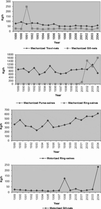
Figure A1. Catch per unit effort by different fishing techniques for marine fish catch in Kerala, 1989–2004.
Appendix B: Biological maximum sustainable regime solution
B1. MSY Solution
The MSY level of effort is derived by modifying the sustainable yield function. The logistic growth function is
and the Gordon–Schaefer fish production function is
In equilibrium,
and so
The sustainable yield function can be written as
By differentiating equation (A3) with respect to effort, setting the derivative to zero and solving for effort, we obtain:
The associated levels of stock and harvest are calculated by setting the derivative of the logistic growth function, with respect to X, to zero:
Finally, substituting the value of X msy in equation (A2) in the sustainable yield equation gives


