


1. Introduction
A finite resistance against the flow is the hallmark of yield stress fluids (YSF): these materials behave like a solid when the applied shear is less than a threshold value (the yield stress) and flow beyond this limit. The prevalence of YSF in food, cosmetics and oil industries (to name a few) has motivated extensive studies to characterize their physical behaviour (Bonn et al. Reference Bonn, Denn, Berthier, Divoux and Manneville2017), the development of different models to describe their rheology (Dinkgreve et al. Reference Dinkgreve, Paredes, Denn and Bonn2016; Bonn et al. Reference Bonn, Denn, Berthier, Divoux and Manneville2017) and experimental and theoretical studies to predict and prescribe their fluid dynamics (Balmforth, Frigaard & Ovarlez Reference Balmforth, Frigaard and Ovarlez2014; Coussot Reference Coussot2014). The ultimate goal remains establishing the link between the rheological tests and models, the theoretical predictions and the experimental observations.
The first and most commonly used model for YSF is the Bingham model. The model assumes the material to be rigid under shear stress less than the yield stress ( $\tau _y$), and fluid with a constant viscosity,
  $\mu$, when the applied shear stress is higher than the yield stress,
 \begin{equation} \left. \begin{array}{lll@{}} \dot{\gamma} = 0 & \tau \le \tau_y & (\text{solid regime}),\\ \tau = \tau_y + \mu \dot{\gamma} & \tau>\tau_y & (\text{fluid regime}). \end{array} \right\} \end{equation}
Here,  $\tau$ and
  $\dot {\gamma }$ are the shear stress and strain rate amplitudes.
Although the Bingham model is extensively used in theoretical studies, its application is limited when it comes to the quantitative rheological description of real materials (Balmforth et al. Reference Balmforth, Frigaard and Ovarlez2014). It is more common to use the Herschel–Bulkley model to describe the steady flow curve of YSF. The model is similar to the Bingham model in assuming an idealized rigid subyield behaviour followed by an instantaneous transition from solid regime to fluid regime. The fluid regime, however, is characterized by a power-law relation in the Herschel–Bulkley model,  $\tau = \tau _y + K \dot {\gamma }^n$. Here,
  $K$ and
  $n$ are the consistency coefficient and the power-law index, respectively.
Although there is general agreement about the practical usefulness of the idea (Nguyen & Boger Reference Nguyen and Boger1992), the existence of a true yield stress fluid has been debated at least since Barnes & Walters (Reference Barnes and Walters1985). This is closely connected to whether and how the yield stress can be measured accurately and used in connection with experimental investigations of fluid dynamics. The difficulties in measuring the yield stress have contributed to the introduction of static and dynamic yield stresses, characteristic of the transition from the solid regime to the fluid regime, and vice versa (Moller et al. Reference Moller, Fall, Chikkadi, Derks and Bonn2009). Simple yield stress fluids (SYSF) are characterized by a viscosity that depends on the shear rate only and have similar static and dynamic yield stresses (Ovarlez et al. Reference Ovarlez, Cohen-Addad, Krishan, Goyon and Coussot2013; Balmforth et al. Reference Balmforth, Frigaard and Ovarlez2014; Coussot Reference Coussot2014). Nevertheless, Dinkgreve et al. (Reference Dinkgreve, Paredes, Denn and Bonn2016) demonstrated that the value of the yield stress can vary significantly depending on the measurement technique.
SYSF primarily include foams, concentrated emulsions and carbopol microgels. Carbopol microgels are widely accepted as SYSF and their flow curve is well described by the Herschel–Bulkley model. The flow curve represents the steady shear stress vs. shear rate. In practice, it is often estimated by conducting stress- or shear-rate-controlled ramps. This includes a finite wait time,  $t_w$, per datapoint. Putz & Burghelea (Reference Putz and Burghelea2009) conducted stress-controlled ramps with
  $0.2\ \mathrm {s} < t_w < 2\ \mathrm {s}$ and observed a systematic hysteresis in the flow curve upon increasing and decreasing the applied stress. This was associated with the solid–fluid transition of the material. The hysteresis was later also observed in shear-controlled sweeps (Divoux, Barentin & Manneville Reference Divoux, Barentin and Manneville2011; Divoux, Grenard & Manneville Reference Divoux, Grenard and Manneville2013). In both cases, the hysteresis decreases as
  $t_w$ increases, suggesting that the hysteresis is a feature of the stress or strain rate ramp tests and not the true flow curve, which corresponds to the steady state. This can be supported by the experiments of Coussot et al. (Reference Coussot, Tocquer, Lanos and Ovarlez2009) and Divoux et al. (Reference Divoux, Tamarii, Barentin, Teitel and Manneville2012), where the velocimetry of steady flow of carbopol microgels in a cylindrical Couette configuration corroborated the theoretical velocity profile based on the Herschel–Bulkley model.
Various key features including flow onset, arrest and instability, however, are not associated with the steady state. Transient flow dynamics has revealed complex events that are not well explained by viscoplastic models (see for example Coussot et al. Reference Coussot, Nguyen, Huynh and Bonn2002a). Coussot et al. (Reference Coussot, Raynaud, Bertrand, Moucheront, Guilbaud, Huynh, Jarny and Lesueur2002b) noted a viscosity bifurcation in YSF in stress-controlled rheometry (see Balmforth et al. Reference Balmforth, Frigaard and Ovarlez2014 for viscosity bifurcation in carbopol microgels). Creep tests, along with time-resolved velocimetry, have unravelled different stages of the development of steady viscometric flows from an initially motionless state.
In both stress-controlled and shear-rate-controlled experiments, with smooth or rough walls, carbopol microgels go through a combination of creep deformation, total wall slip and shear banding before a homogenous flow is established (Divoux et al. Reference Divoux, Tamarii, Barentin and Manneville2010, Reference Divoux, Barentin and Manneville2011). In strain rate (stress) controlled experiments, the fluidization time,  $t_f$, decreases as a power law of the shear rate (the difference between the applied stress and the yield stress). The fluidization time thus approaches infinity close to the theoretical yield condition,
  $\dot {\gamma }=0$ or
  $\tau =\tau _y$; for obvious practical reasons, the largest measured values are approximately 20–30 h (Divoux et al. Reference Divoux, Tamarii, Barentin and Manneville2010). Expectedly, fluidization process and
  $t_f$ depend on the imposed (stress or shear rate) condition and the flow geometry (Divoux et al. Reference Divoux, Tamarii, Barentin, Teitel and Manneville2012).
When the applied shear stress is below the yield stress, solid-like creep deformation has been observed in different viscometric flows (Coussot et al. Reference Coussot, Nguyen, Huynh and Bonn2002a, Reference Coussot, Tabuteau, Chateau, Tocquer and Ovarlez2006; Divoux et al. Reference Divoux, Barentin and Manneville2011; Balmforth et al. Reference Balmforth, Frigaard and Ovarlez2014; Lidon, Villa & Manneville Reference Lidon, Villa and Manneville2017). Here, a transient creep deformation regime arises that develops as a power law of time before the motionless state is recovered. Consistently, when the loading condition of the system changes, the system goes through a series of transient states before a new (and possibly different) steady state is established.
An indisputable majority of the theoretical and numerical studies on YSF are based on the Herschel–Bulkley and Bingham models (hereafter referred to as viscoplastic models). The notions of rigidity below the yield stress and instantaneous fluidization are inherent to viscoplastic models and, consequently, to theoretical studies of fluid dynamics of SYSF. Mathematical and numerical studies based on viscoplastic models predict various key features of flows of SYSF. Typically, the yield stress has to be below a critical value to ensure the existence of a steady flow (see for example Mosolov & Miasnikov Reference Mosolov and Miasnikov1966). Above the critical yield stress, the motionless state is often linearly stable and perturbations decay to zero within a finite time (Bristeau Reference Bristeau1975; Glowinski, Lions & Trémolières Reference Glowinski, Lions and Trémolières1981).
The conditions necessary to suppress internal natural convection of viscoplastic fluids (the critical condition) have been investigated in different classical problems (Yang & Yeh Reference Yang and Yeh1965; Lyubimova Reference Lyubimova1977; Karimfazli, Frigaard & Wachs Reference Karimfazli, Frigaard and Wachs2016). Zhang, Vola & Frigaard (Reference Zhang, Vola and Frigaard2006) showed that the motionless background state in the Rayleigh–Bénard setting is linearly stable and velocity disturbances decay to zero in a finite time. They also provided stability bounds for the motionless background state. Karimfazli & Frigaard (Reference Karimfazli and Frigaard2016) characterized the sufficient conditions for steady natural convection in viscoplastic fluids. When the buoyancy stress is irrotational, the steady state may be motionless irrespective of the value of the yield stress. When the buoyancy stress is rotational, there is a critical ratio of the yield stress and buoyancy stress ( $B_{cr}$), below which the steady state is convecting.
Typically, the temperature field evolves by conduction and advection before reaching the steady state. The time evolution of the temperature field indicates that buoyancy stress is similarly time dependent. Karimfazli & Frigaard (Reference Karimfazli and Frigaard2016) demonstrated that a time-dependent Bingham number ( $b(t)$), defined based on the instantaneous buoyancy stress, determines the flow onset time. In particular, when
  $b(0)>B_{cr}$ and buoyancy increases with time, natural convection starts at the earliest time
  $t_0>0$ that
  $b(t_0)=B_{cr}$; i.e. flow onset may be delayed by a finite time.
Experimental realizations of the predicted flow features are strikingly limited in comparison with the abundance of theoretical and numerical studies. Darbouli et al. (Reference Darbouli, Métivier, Piau, Magnin and Abdelali2013) and Kebiche, Castelain & Burghelea (Reference Kebiche, Castelain and Burghelea2014) studied Rayleigh–Bénard convection of carbopol microgel and identified steady convective currents by comparing the temperature difference across the cell with the purely conductive case. Although their findings were not in qualitative agreement, both reported the development of steady flow from a motionless background state at sufficiently large temperature differences. This is in apparent contradiction with the theoretical findings on the stability of the motionless background state in SYSF. Another experimental study by Davaille et al. (Reference Davaille, Gueslin, Massmeyer and Di Giuseppe2013) considered the development of thermal plumes in carbopol microgels. They reported a critical yield stress above which no flow was observed. Their observations were later rationalized using viscoplastic models (Karimfazli et al. Reference Karimfazli, Frigaard and Wachs2016).
Quantitative discrepancies between the experiments and theoretical predictions may be associated with the difficulties of measuring the yield stress accurately or creating ideal boundary conditions in experiments. Phenomenological differences, however, hint at shortcomings in the theoretical models. In this work, we examine the accuracy of viscoplastic models in predicting motion development in SYSF. We present a phenomenological comparison of experimental observations and theoretical predictions of internal buoyancy-driven flows. We inspect motion development patterns for manifestations of fluidization or subyield motion. We aim to reveal the limitations of viscoplastic models in predicting unsteady flows of SYSF.
We consider the development of natural convection in a square cavity with differentially heated sidewalls, filled with a carbopol microgel initially at rest and room temperature. This is analogous to the two-dimensional problem studied by Karimfazli & Frigaard (Reference Karimfazli and Frigaard2016), where the fluid is initially motionless and at the reference temperature. We evaluate two primary theoretical predictions (i) the existence of a critical yield stress above which steady flow is completely suppressed (Lyubimova Reference Lyubimova1977; Turan, Chakraborty & Poole Reference Turan, Chakraborty and Poole2010; Vikhansky Reference Vikhansky2010; Karimfazli, Frigaard & Wachs Reference Karimfazli, Frigaard and Wachs2015), and (ii) delayed onset of natural convection (Karimfazli & Frigaard Reference Karimfazli and Frigaard2016).
The experimental set-up and methodology are described in § 2. In § 3 we examine the existence of the critical yield stress and develop intuitive quantitative characteristics to reveal motion onset time and the pursuing dynamics. We close in § 4 by presenting our concluding remarks.
2. Experimental set-up and methodology
2.1. Experiment set-up
The experimental set-up is illustrated in figure 1. It consists of a cubic cell of size  $L=14.6\ \mathrm {cm}$, with the top, bottom, front and back walls built from acrylic sheets of thickness
  $25.4\ \mathrm {mm}$. The sidewalls are made of
  $12.7\ \mathrm {mm}$ thick sheets of aluminium to facilitate heat transfer. Two thermoelectric modules (TEMs) are used to maintain the sidewalls at specific high and low temperatures,
  $T_H$ and
  $T_L$ respectively. These modules have the same surface area as the sidewalls of the cavity. They were attached to the aluminium walls to provide a uniform temperature on the sidewalls. During the experiment, the temperature of each module was maintained using a temperature controller that works based on feedback control and adjusts the heating and cooling power of the unit based on its temperature. Two thermocouples (type
  $T$) were mounted on either side, between the TEM and the aluminium sidewall, to monitor the development of the temperature on the walls throughout the experiments. The thermocouples were mounted at the middle and top corner of each wall. The difference between the two measurements on each side provides an approximation of the maximum temperature variation on each sidewall.

Figure 1. Experimental set-up. Each sidewall of the cavity is attached to a thermoelectric module (TEM). The modules are turned on at  $t=0$ and maintain the walls at the preset temperatures through feedback control.
All experiments started with the working fluid at rest and the set-up at room temperature ( $T_r = 24 \pm 1\, ^{\circ }\mathrm {C}$). Each carbopol microgel was tested subject to a range of temperature differences across the cavity,
  $5\, ^{\circ }\mathrm {C} \lesssim \Delta T \lesssim 30\, ^{\circ }\mathrm {C}$. The TEMs were turned on and data acquisition started at
  $t=0$. Data collection continued until flow was considered steady (see more details in § 2.3).
2.2. Fluids
Aqueous solutions of carbopol were prepared by mixing carbopol ETD2050 with distilled water. First carbopol powder ( $0.35\text {--}0.40\ \mathrm {g}\,\mathrm {l}^{-1}$) was slowly added to the solvent (distilled water) and mixed with a mechanical mixer at
  $600\ \mathrm {rpm}$ until homogeneous. The solution was then neutralized to
  $\textrm {pH}=7$ using a few microlitres of
  $5\ \mathrm {M}$ sodium hydroxide.
The flow curves of the solutions were measured after adding the seeding particles. The tests were conducted at room temperature using a DHR-3 rheometer. Each sample was tested a minimum of three times to ensure the repeatability of the measured flow curve. Figure 2 illustrates the average curve for each sample along with the standard deviations. In our experiments, the fluid temperature varied from approximately  $8$ to
  $40\, ^{\circ }\mathrm {C}$ to avoid the risk of freezing or significant evaporation. The sidewall temperatures where chosen such that the reference temperature was
  $T_o=(T_H+T_L)/2=24\pm 1\, ^{\circ }\mathrm {C}$ for all experiments. Although rheological features of carbopol microgels are temperature dependent, the relative change of these properties, over the temperature ranges considered here, is not significant (see Weber, Moyers-González & Burghelea (Reference Weber, Moyers-González and Burghelea2012) and the references therein).

Figure 2. Flow curves of the carbopol microgels (a)  $c=0.35\ \mathrm {g}\,\mathrm {l}^{-1}$, (b)
  $0.38\ \mathrm {g}\,\mathrm {l}^{-1}$, (c)
  $0.4\ \mathrm {g}\,\mathrm {l}^{-1}$. The circle markers show the measured flow curved, averaged over multiple tests. The error bars indicate the standard deviation of the measurements. The red dashed lines show the fitted Herschel–Bulkley model for each sample. The corresponding rheological parameters are tabulated in table 1.
Table 1. Rheological parameters of working fluids at  $T_o=24\, ^{\circ }\mathrm {C}$:
  $c$,
$c$,  $\tau _y$,
  $K$ and
  $n$ represent the concentration, yield stress, consistency and power-law index, respectively.

There are various methods to measure the yield stress (Coussot Reference Coussot2014). In the context of the Herschel–Bulkley model, the yield stress and other rheological parameters of the model are found by fitting the constitutive law to the flow curve (see e.g. Divoux et al. Reference Divoux, Tamarii, Barentin and Manneville2010; Hormozi, Martinez & Frigaard Reference Hormozi, Martinez and Frigaard2011; Chevalier et al. Reference Chevalier, Chevalier, Clain, Dupla, Canou, Rodts and Coussot2013; Darbouli et al. Reference Darbouli, Métivier, Piau, Magnin and Abdelali2013; Davaille et al. Reference Davaille, Gueslin, Massmeyer and Di Giuseppe2013). We follow the same procedure, fitting the Herschel–Bulkley model to the range  $10^{-2}\le \dot {\gamma } \le 1$. The rheological parameters are shown in table 1.
Due to the very low mass concentration of carbopol, we use density and thermal properties of water at the reference temperature to estimate the dimensionless variables explored by the experiments
 \begin{equation} \left. \begin{array}{ll@{}} \rho = 997 \ \mathrm{kg}\,\mathrm{m}^{-3} & \alpha = 0.14(10^{-6}) \ \mathrm{m}^2\,\mathrm{s}^{-1},\\ \beta = 0.237(10^{-3})\, ^{\circ}\mathrm{C}^{-1} & c_p = 4180 \ \mathrm{J}\,(\mathrm{kg}\,\mathrm{K})^{-1}. \end{array} \right\} \end{equation}
Here,  $\rho$ is the density,
  $\alpha$ is the thermal diffusivity,
  $\beta$ is the volume expansion coefficient and
  $c_p$ is the specific heat. Carbopol microgels have very large Prandtl numbers,
  $Pr\gg 1$. The other two dimensionless parameters relevant to natural convection of viscoplastic fluids are the Bingham number,
 \begin{equation} B=\frac{\tau_y}{\rho g L \beta \Delta T}, \end{equation}
and the effective Rayleigh number,
 \begin{equation} Ra_e =\frac{L^2/\alpha}{L/U}. \end{equation}
Here,  $g$ is the acceleration due to gravity,
  $U$ is the characteristic velocity of the steady flow and
  $\Delta T=T_H-T_L$ is the temperature difference between the two sidewalls.
Using Boussinesq assumption and neglecting the variation of fluid properties with temperature, the critical Bingham number in two-dimensional square cavities has been predicted using scaling analysis (Lyubimova Reference Lyubimova1977), numerical simulations (Vikhansky Reference Vikhansky2009; Turan et al. Reference Turan, Chakraborty and Poole2010) and asymptotic analysis (Karimfazli et al. Reference Karimfazli, Frigaard and Wachs2015),  $B_{cr}=1/32$. When the Bingham number is higher than the critical value, the steady state is predicted to be motionless.
Based on the size of the cavity and the fluid properties at the reference temperature, at our maximum temperature difference of  $30\, ^{\circ }\mathrm {C}$ the critical Bingham number corresponds to a yield stress of approximately
  $0.22\ \mathrm {Pa}$; i.e. when
  $\tau _y=0.22\ \mathrm {Pa}$, we do not expect to observe steady flow even at the highest
  $\Delta T$. Another limitation on the yield stress in natural convection experiments is that, assuming a uniform temperature at time zero, the flow onset time approaches infinity close to the critical condition (Karimfazli & Frigaard Reference Karimfazli and Frigaard2016; Karimfazli et al. Reference Karimfazli, Frigaard and Wachs2016). The largest yield stress used in our experiments, therefore, is
  $\tau _y=0.16\ \mathrm {Pa}$ (see table 1). The Bingham numbers of the experiments were
  $0.004 \lesssim B \lesssim 0.03$ while the effective Rayleigh numbers were
  $0 \lesssim Ra_{e} \lesssim 700$.
2.3. Flow characterization methodology
Our flow visualization method is quite similar to the method used by Davaille et al. (Reference Davaille, Gueslin, Massmeyer and Di Giuseppe2013). The fluid was seeded with a thermochromic liquid crystal slurry, TLC. The vertical symmetry plane of the cell was illuminated using a  $532\ \mathrm {nm}$ laser sheet. When illuminated with a
  $532\ \mathrm {nm}$ laser, the TLC reflects light at a certain temperature, revealing an isotherm within the flow domain. To identify this temperature, we conducted experiments where the fluid remains motionless and the temperature develops purely conductively. Here, the steady temperature field is described by a linear profile between the two sidewalls. The isotherm is a vertical line that appears close to one of the walls (figure 3a,c) and then moves toward its steady position exponentially. The location of the isotherm can be found by image analysis and locating the peak intensity (figure 3a,c). We used an exponential fit to the position of the isotherm to find the steady position of the vertical line and the corresponding temperature,
  $T_i = 27.2\, ^{\circ }\mathrm {C}$ (figure 3b).

Figure 3. TLC calibration. (a,c) A snapshot of the experiment at  $t=6\ \mathrm {h}$ (a) and the corresponding normalized light intensity as a function of position (c). (b) The time evolution of the position of the isotherm. The solid red line is a fitted exponential curve and the dashed red line is the steady position of the isotherm.
TLC aggregates also serve as tracing particles, revealing the temporal evolution of the flow using time-resolved particle image velocimetry (PIV). For all experiments, images were recorded every  $4\ \mathrm {s}$ using a CCD camera. The cross-correlation times used varied from
  $20\ \mathrm {s}$ to
  $500\ \mathrm {s}$ and were chosen a posteriori based on the observed velocity magnitudes for each experiment. The PIV analyses were conducted using a customized MATLAB program based on PIVLab (Thielicke & Stamhuis Reference Thielicke and Stamhuis2014). Of particular interest here was to identify flow onset time and to reveal the early dynamics during the flow onset. Darbouli et al. (Reference Darbouli, Métivier, Piau, Magnin and Abdelali2013) and Kebiche et al. (Reference Kebiche, Castelain and Burghelea2014) used the Schmidt–Milverton principle (Schmidt & Milverton Reference Schmidt and Milverton1935) to identify the presence of steady advection in viscoplastic fluids in the Rayleigh–Bénard setting. This approach is based on a steady-state heat transfer analysis. It is therefore not suitable for resolving unsteady velocity field features, including motion onset. We use time-resolved PIV together with particle trajectories to characterize flow features at flow onset when advection is extremely weak and heat transfer appears purely conductive.
To characterize flow onset we use the average velocity,  $\bar {v}$, representative of the flow rate in the symmetry plane of the cavity
 \begin{equation} \bar{v} =\frac{2}{L}\int_{L/2}^{L}v(x,y=L/2,z=L/2)\,{\textrm{d}x}. \end{equation}
Here,  $v$ is the vertical component of the velocity. See figure 1 for a schematic of the flow domain and the coordinate system. We use particle trajectories along with the time evolution of
  $\bar {v}$ to confirm structured motion in the cavity. To distinguish systematic fluid motion from motionless states, we conducted a benchmark experiment. We followed the same procedure as the other experiments with the exception that no heating and cooling was imposed on the sidewalls. Figure 4 shows the particle trajectories and
  $\bar {v}$ for the benchmark experiment. Figure 4(b,c) illustrates the time evolution of
  $\bar {v}$ with time. Here,
  $\bar {v}$ has a normal distribution around zero (see figure 4d), which confirms the absence of systematic motion in the benchmark experiment. The cross-correlation of the images, therefore, should be independent of the cross-correlation time,
  $t_{cc}$. This is confirmed by noting that the standard deviation of
  $\bar {v}$ is inversely proportional to the
  $t_{cc}$ (figure 4e). Because the data have a normal distribution,
  $99\,\%$ of values fall within 2.58 standard deviations of the mean. For a given
  $t_{cc}$, the corresponding
  $99\,\%$ confidence interval (
 $CI_{99}$) of this benchmark experiment is used to identify the motionless state. On the other hand, the presence of motion is confirmed when the value of
  $\bar {v}$ exceeds
  $CI_{99}$. It should be noted, however, that we cannot resolve the velocity field of all such flowing states. When the signal to noise ratio is low, i.e.
  $(\bar {v}/CI_{99}) = O(1)$ our PIV results appear noisy. In such cases, velocity measurements are accompanied by illustrations of particle trajectories to reveal the flow dynamics.

Figure 4. Benchmark experiment measurements. (a) Particle pathlines  $0 < t < 2\ \mathrm {h}$. (b,c) The evolution of the
  $\bar {v}$ using
  $t_{cc}=20\ \mathrm {s}$ (b) and
  $400\ \mathrm {s}$ (c). (d) Histogram of
  $\bar {v}$ for
  $t_{cc}=20\ \mathrm {s}$. The solid red line illustrates the normal distribution fit. (e) Standard deviation of
  $\bar {v}$ vs. cross-correlation time. The red line represents an inverse fit,
  $SD=a/t_{cc}$.
Finally, the experimental approach is validated by conducting repeatability tests. Figure 5 illustrates the evolution of the  $L^2$ norm of the velocity field,
 \begin{align} ||u||=\sqrt{\int_0^L\int_0^L \left|\mathbf{u}(x,y=L/2,z)\right|^2 {\rm d}x\ {\rm d}z}, \end{align}
and  $\bar {v}$ and the corresponding standard deviations of the time-resolved PIV results. The dashed lines indicate the corresponding
  $CI_{99}$.

Figure 5. Repeatability test outcomes for (a,b)  $c=0.35\ \mathrm {g}\,\mathrm {l}^{-1}$,
  $\Delta T =31.0\, ^{\circ }\mathrm {C}$,
  $t_{cc}=20\ \mathrm {s}$ and (c,d)
  $c=0.38\ \mathrm {g}\,\mathrm {l}^{-1}$,
  $\Delta T =31.9\, ^{\circ }\mathrm {C}$,
  $t_{cc}=500\ \mathrm {s}$. The grey area shows the standard deviation of the data. The dashed blue line indicates the corresponding
  $CI_{99}$.
3. Results and discussions
Depending on the yield stress of the fluid and the imposed temperature difference, a steady flow is established in the cavity; figure 6 shows an illustrative case. We use the  $L^2$ norm of the velocity field,
  $||u||$, to show the development of the kinetic energy in the domain. The velocity norm initially increases slowly, before accelerating, reaching an absolute maximum and decaying to the steady state (see figure 6a). The overall flow development pattern appears similar to the theoretical predictions based on the Bingham model (Karimfazli et al. Reference Karimfazli, Frigaard and Wachs2015). Figures 6(b), 6(c) and 6(g) show snapshots of the velocity magnitude during the flow evolution. The apparent noise in the velocity measurements on the top wall is related to the optical interference of the fastenings used to attach the top lid to the cell. Figure 6(b) suggests that flow starts on the hot (right) wall. This is because TEMs have a higher heating capacity compared to their cooling capacity: heat transfer on the hot side is higher during the initial transition to the steady wall temperature. The evolution of the temperature on the walls is illustrated in figure 6(d). Note that the wall temperatures reach the steady state significantly faster than the flow field. In all experiments, the temperature non-uniformity on each wall decreases with time and is less than
  $1.5\, ^{\circ }\mathrm {C}$ once the temperatures are steady. Figures 6(e), 6(f) and 6(h) illustrate the evolution of the temperature field in the domain. The dark lines show the instantaneous shape of the isotherm
  $T=27.2\, ^{\circ }\mathrm {C}$.

Figure 6. Illustration of the velocity and temperature data;  $c=0.35\ \mathrm {g}\,\mathrm {l}^{-1}, \Delta T= 21.9\, ^{\circ }\mathrm {C}$. (a) Evolution of the velocity norm with time. (b,c,g) Snapshots of the velocity field (in
  $\ \mathrm {mm}\,\mathrm {s}^{-1}$). (d) Evolution of the temperature of the hot and cold walls. There are two thermocouples on each wall, one at the centre (the black curves) and one at the top corner (the blue curves). The difference between the two sensors on each wall is representative of the maximum temperature variation on the wall. (e,f,h) Snapshots of the isotherm
  $T=27.2\, ^{\circ }\mathrm {C}$. The red markers in (a,d) indicate the times when the snapshots are taken. Times are (b)
  $t=0.57\ \mathrm {h}$. (c)
  $t=1.10\ \mathrm {h}$. (e)
  $t=0.57\ \mathrm {h}$. (f)
  $t=1.10\ \mathrm {h}$. (g)
  $t=2.78\ \mathrm {h}$. (h)
  $t=2.78\ \mathrm {h}$.
3.1. The critical condition
Figure 7(a) illustrates the flow development for  $c=0.35\ \mathrm {g}\,\mathrm {l}^{-1}$ and
  $4.9\, ^{\circ }\mathrm {C} \leq \Delta T \leq 31.0\, ^{\circ }\mathrm {C}$. As
  $\Delta T$ decreases, the steady-state velocity norm decreases. To better distinguish steady flow and motionless steady state, the time evolution of
  $\bar {v}$ is illustrated in figures 7(b)–7(d). At
  $\Delta T=4.9\, ^{\circ }\mathrm {C}$, although some transient motion exists,
  $\bar {v}$ decays toward the motionless state and steady flow is not established (steady flow is confirmed when
  $\bar {v}$ approaches a steady value that exceeds
  $CI_{99}$). More details about this transient motion are presented in §§ 3.2 and 3.3.

Figure 7. (a) Evolution of the velocity norm,  $c=0.35\ \mathrm {g}\,\mathrm {l}^{-1}$ and different
  $\Delta T$. (b–d) Time evolution of
  $\bar {v}$. The blue dashed line in (b–d) indicates
  $CI_{99}$ for the corresponding
  $t_{cc}$. The cross-correlation times used for
  $\Delta T=(4.9, 14.4, 21.9, 26.5, 31.0)\, ^{\circ }\mathrm {C}$ are
  $t_{cc}= (500, 100, 20, 20, 20)\ \mathrm {s}$.
The critical condition is the condition differentiating steady flow and motionless steady states. Presence of the steady motionless state, and thus the critical condition, depends on the ratio of buoyancy and yield stresses captured by the Bingham number. Figure 8 illustrates the flowing and motionless states for different yield stress and temperature difference values. The grey area separates the flowing and motionless steady states. The markers above (below) this region indicate the experiments where the steady state was motionless (flowing). Our experimental results, therefore, bound the critical Bingham number within the grey region;  $B_{cr}=0.012\pm 0.002$. Both experimental and theoretical critical conditions depend on the ratio of the buoyancy and yield stresses; although the theoretical value,
  $B_{cr}=1/32$, is an overestimation compared with the experimental one.

Figure 8. Illustration of the critical condition. The filled and empty markers indicate motionless and flowing steady states, respectively. Buoyancy stress is estimated as  $\rho g \beta L \Delta T$. The grey area indicates the upper and lowers bounds of the critical condition. The solid line represents the estimated critical condition,
  $B_{cr} \approx 0.012 \pm 0.002$.
A key difference between the theoretical and experimental problem is the Boussinesq approximation: the theoretical studies neglect variation of all fluid properties with temperature except in evaluating the buoyancy stresses. While the yield stress, density and thermal diffusivity may not change significantly over the temperature ranges considered here, the volume expansion coefficient changes by approximately  $100\,\%$. Presence of wall slip in the experiments, in contrast with the presumed no-slip condition in theoretical studies, can also contribute to the observed differences (Darbouli et al. Reference Darbouli, Métivier, Piau, Magnin and Abdelali2013). The neglected temperature dependence of material properties and the possibility of wall slip, together with the uncertainties associated with evaluating the yield stress, can justify the difference between the theoretical and experimental
  $B_{cr}$.
3.2. Flow development from the motionless initial state
Viscoplastic models assume motion is completely suppressed until the applied shear stress exceeds the yield stress. In our experiments, the fluid is initially motionless and at room temperature. This is analogous to the problem studied by Karimfazli & Frigaard (Reference Karimfazli and Frigaard2016): at  $t=0$ the fluid temperature is uniform and the buoyancy stresses are, thus, zero. As the temperature field evolves, buoyancy stresses grow proportional to the variation of the density in the flow domain. Because the fluid has a non-zero yield stress, and the buoyancy stresses grow continuously with time, a finite time delay is necessary for buoyancy stresses to grow and exceed the yield stress.
There are also marked differences between the theoretical and experimental boundary conditions. Firstly, the target temperature is not established instantaneously on the sidewalls. Secondly, the top and bottom walls are not perfectly insulated. Therefore, the steady state is realized on a longer time scale compared to the theoretical predictions. The difference between the theoretical and experimental flow fields decreases as the steady state is approached.
Figure 9 shows a few illustrative cases of the evolution of velocity norm and  $\bar {v}$, representative of all experiments with flowing steady states. Velocity norm initially changes negligibly and remains close to zero before increasing more rapidly (see figure 9(a–c) when
  $t \lesssim 0.1\ \mathrm {h}$). In all cases, however, comparison of
  $\bar {v}$ with
  $CI_{99}$ after the start of the experiments reveals no evident delay in motion development (see figure 9d–f).

Figure 9. Evolution of the (a–c) velocity norm and (d–f) average velocity,  $c=0.35\ \mathrm {g}\,\mathrm {l}^{-1}, t_{cc} =60\ \mathrm {s}$. The dashed lines represent
  $CI_{99}$ with (a,d)
  $\Delta T=31.0\, ^{\circ }\mathrm {C}$. (b,e)
  $\Delta T=26.5\, ^{\circ }\mathrm {C}$. (c,f)
  $\Delta T=21.9\, ^{\circ }\mathrm {C}$.
Theoretical analysis based on viscoplastic models show that flow onset time,  $t_o$, is a function of the Bingham number (Karimfazli & Frigaard Reference Karimfazli and Frigaard2016),
 \begin{equation} t_{o} = \left(\frac{L^2}{\alpha}\right) f(B) \end{equation}
and that it approaches infinity close to the critical condition,  $\lim _{B\rightarrow B_{cr}^-} t_o = +\infty$. Critically, this prediction is based on the assumption that the material remains rigid below the yield stress. Consistent with this prediction, the latest emergence of viscoplastic flow in our experiments corresponds to the lowest
  $B_{cr}-B>0$, i.e.
  $c=0.38\ \mathrm {g}\,\mathrm {l}^{-1}$,
  $\Delta T=31.9\, ^{\circ }\mathrm {C}$ (figure 10). Here, immediate motion onset and slow decay are evident (figure 10a and 10c,
  $t \lesssim 1.4 \ \mathrm {h}$) before the appearance of viscoplastic flow patterns.

Figure 10. Illustration of (a) the velocity norm and (c) average velocity at  $c=0.38\ \mathrm {g}\,\mathrm {l}^{-1}, \Delta T= 31.9\, ^{\circ }\mathrm {C}$,
  $t_{cc}=500\ \mathrm {s}$. (b,d) Snapshots of the velocity field (in
  $\ \mathrm {mm}\,\mathrm {s}^{-1}$). The red markers in (a,c) indicate the times when the snapshots are taken. (e) Evolution of the temperature of the hot and cold walls. There are two thermocouples on each wall, one at the centre (the black curves) and one at the top corner (the blue curves). (f) Particle pathlines during the initial slow development (before the first snapshot). Times are (b)
  $t=1.4\ \mathrm {h}$. (d)
  $t=9\ \mathrm {h}$. (f)
  $0 < t < 1.4\ \mathrm {h}$.
Predictions based on viscoplastic models also indicate that, if motion remains negligible and heat transfer is primarily conductive, shear stresses in the domain do not exceed the yield stress and the material remains in the solid regime (i.e.  $\tau \le \tau _y$) for
  $t < t_o$. Since motion is extremely slow during the initial phase, we speculate that the fluid regime is not yet established. This hypothesis is supported by noticing that there are no distinct unyielded regions during this phase (see figure 10b). This is in contrast with the steady state, where unyielded regions can be identified at the corners of the cavity (see figure 10d). Note that, although the velocity magnitudes are quite small, particle pathlines confirm structured fluid motion during the initial stage (figure 10f).
The immediate motion onset characterized by a distinct initial jump is ubiquitous in our experiments. The initial jump in  $\bar {v}$ followed by a slow decay are reminiscent of the events observed by Divoux et al. (Reference Divoux, Barentin and Manneville2011) and Lidon et al. (Reference Lidon, Villa and Manneville2017). Initially, the shear stress remains below the yield stress everywhere in the domain. We thus characterize the slow decay as creep behaviour. Flow confinement and the spatial and temporal variation of the shear stress, however, prevent the appearance of a power-law decay with time. As the buoyancy stresses increase and shear stress exceeds the yield stress in parts of the domain, fluidization starts. Due to heterogeneity of the shear stress, however, the fluidization is asynchronous across the domain. Velocity norm and
  $\bar {v}$ represent the accumulative evolution of all these events with time. After the initial slow dynamics, flow development patterns are analogous to the theoretical predictions based on the Bingham model Karimfazli et al. (Reference Karimfazli, Frigaard and Wachs2015) (hereafter referred to as viscoplastic flow patterns).
3.3. Subyield motion
At yield stress values above the critical limit, temperature evolves primarily conductively throughout the experiment and buoyancy stresses increase as the steady state is approached. Nevertheless, buoyancy stress is not sufficient to promote a steady flow. Viscoplastic models predict no systematic motion throughout the experiment. Contrary to this prediction, we observed the immediate onset of motion in the experiments; a few representative cases are shown in figure 11. Since buoyancy stresses increase with time and the steady state is motionless, we infer that the material remains in the solid regime throughout the experiment.

Figure 11. Evolution of  $\bar {v}$ when the steady state is motionless (a,c,e). The red markers indicate the time at which a snapshot of the velocity is illustrated (b,d,f). Parameters are (a,b)
  $c=0.35\ \textrm{g}\ {\rm l}^{-1}, \Delta T=4.9\, ^{\circ }\mathrm {C}$, (c,d)
  $c=0.38\ \mathrm {g}\,\mathrm {l}^{-1}, \Delta T=14.6\, ^{\circ }\mathrm {C}$, (e,f)
  $c=0.38\ \mathrm {g}\,\mathrm {l}^{-1}, \Delta T=22.4\, ^{\circ }\mathrm {C}$ and
  $t_{cc}=400\ \mathrm {s}$ for all cases. The dashed lines represent
  $CI_{99}$. The vertical bright lines in (d,f) are due to the interference of the isotherm.
Consistently, an initial jump in  $\bar {v}$ is followed by extremely slow and approximately linear decay (see figure 11a,c,e). Assuming that the deformation rate is of order
  $\bar {v}/L$, the evolution of
  $\bar {v}$ directly reflects that of the deformation rate. It suggests that the material deforms rapidly at first (see
  $t\lesssim 1\ \mathrm {h}$ in figure 11), before the deformation rate decays over a much longer time interval (see
  $t>1\ \mathrm {h}$ in figure 11).
Figures 11(b), 11(d) and 11(f) illustrate snapshots of the velocity field at the time instants when the signal to noise ratio is the highest, i.e. close to the maximum of  $\bar {v}$ (the bright vertical lines are due to interference of the isotherm). The velocity fields reveal extremely slow motion that is arguably at the lower limit of our measuring range. We used particle pathlines to confirm immediate motion onset and reveal the motion structure. Figure 12 shows an illustrative case,
  $c=0.38\ \mathrm {g}\,\mathrm {l}^{-1}$,
  $\Delta T=22.4\, ^{\circ }\mathrm {C}$. The pathlines confirm the immediate onset of motion in all cases with motionless steady state. Figures 12(a) and 12(b) illustrate the particle pathlines during the initial jump and the decay of
  $\bar {v}$, respectively. Both development phases reveal counterclockwise circulation of the particles, reminiscent of natural convection in a cavity. Figure 12(a) confirms the slight asymmetry due to the higher heat transfer rate on the hot wall compared to the cold wall. Figure 12(b) also confirms the deceleration of the particles with time as pathlines get darker in the counterclockwise direction.

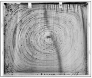
Figure 12. Particle pathlines during (a) the initial jump of the average velocity and (b) the deceleration to rest. Here,  $c=0.38\ \mathrm {g}\,\mathrm {l}^{-1}, \Delta T = 22.4\, ^{\circ }\mathrm {C}$; (a)
  $0 < t < 1.1\ \mathrm {h}$, (b)
  $1.1 < t < 6\ \mathrm {h}$.
In all experiments with motionless steady states, the decay patterns appear approximately linear with time (see e.g. figure 11a,c,e). This decay pattern reveals the non-viscous nature of the observed dynamics: exponential energy decay is the hallmark of viscous energy dissipation. The observed patterns are indicative of an elastic response followed by creep deformation. This is similar to the creep tests of Lidon et al. (Reference Lidon, Villa and Manneville2017) below the yield stress. Expectedly, however, we do not observe the signature power-law creep as, unlike the creep test, the flow domain is confined and the stress field is non-uniform and time dependent.
4. Summary and discussion
We have conducted a systematic study of motion development from a motionless initial state in carbopol microgels. A square cavity filled with carbopol microgels with different concentrations was subjected to a horizontal temperature difference of  $4.9\, ^{\circ }\mathrm {C} \le \Delta T \le 31\, ^{\circ }\mathrm {C}$. For all carbopol concentrations, we observed a threshold temperature difference below which steady flow is not observed. Our experimental estimate of
  $B_{cr}\approx 0.012$ is comparable to the theoretically predicted value for two-dimensional convection in a square cavity with differentially heated sidewalls,
  $B_{cr}=1/32$ (Karimfazli et al. Reference Karimfazli, Frigaard and Wachs2015). The difference is expected due to the uncertainties associated with the measurement of the yield stress, the variation of fluid properties with temperature that is neglected in theoretical studies, the possibility of wall slip in the experiments and the unavoidable differences between the experimental and theoretical boundary conditions.
Careful characterization of the development dynamics revealed the immediate onset of motion in carbopol microgels at the beginning of the experiment (irrespective of how the yield stress compared with the critical value). When the yield stress is above the critical value, material deforms rapidly at first as buoyancy stresses evolve. This is followed by very slow decay of the deformation rate, reminiscent of creep behaviour. These dynamics are representative of the solid regime. This is further verified by noticing that the energy decay is not exponential and, thus, cannot be associated with viscous dissipation. The transient dynamics observed here is similar to that reported by Lidon et al. (Reference Lidon, Villa and Manneville2017). The time evolution of the imposed buoyancy stresses and the confinement of the flow domain, however, prevent a quantitative comparison of the data.
When the steady state is convective, motion starts immediately and evolves very slowly before viscoplastic flow patterns appear. In most of the flowing experiments, the Bingham number is much smaller than the critical value. The buoyancy stresses exceed the yield stress rapidly and the fluidization times are shorter. Temporal and spatial shear stress heterogeneity in the domain indicates that fluidization is asynchronous in the domain. Once the material is partially fluidized, it dominates the development patterns observed as motion and strain rates associated with the solid regime are orders of magnitude smaller than the fluidized regime. The transition between the two regimes is most evident at  $c=0.38\ \mathrm {g}\,\mathrm {l}^{-1}$ and
  $\Delta T=31.9\, ^{\circ }\mathrm {C}$, which corresponds to the smallest
  $0<(B_{cr}-B)$ in our experiments. In this experiment motion initially evolves relatively rapidly as buoyancy stresses in the domain increase. This is followed by a slow creep-like decay before the material is fluidized. After this initial phase, the flow development is similar to the theoretical predictions of Karimfazli et al. (Reference Karimfazli, Frigaard and Wachs2015): a quick rise and a local maximum in kinetic energy are followed by a slight decay and smooth approach to a steady flow.
Experimental observations of the critical condition, distinguishing the motionless and convecting steady states, corroborate the theoretical predictions. Contrary to theoretical predictions, however, motion onset is immediate in all experiments. The seemingly inconsistent connection of the experiments and theory on SYSF may be explained by a key assumption of viscoplastic models, that both the solid and fluid regimes are established instantaneously. Motion onset dynamics are transient events inherently associated with the material response to changes in loading conditions, that is a change in boundary conditions or body forces (buoyancy here). This material response time increases significantly if the imposed conditions are close to the yielding condition (that is  $\dot {\gamma }\rightarrow 0$ or
  $\tau \rightarrow \tau _y$) (Divoux et al. Reference Divoux, Tamarii, Barentin and Manneville2010, Reference Divoux, Barentin and Manneville2011; Lidon et al. Reference Lidon, Villa and Manneville2017). Inevitably, the immediate response of carbopol microgels in our experiments contradicts the predictions based on viscoplastic models; the time scale of the events we have studied here is comparable to the material response time and, thus, steady flow curve is not representative of material behaviour.
Finally, we hypothesize that theory and observations are consistent if the transition between the solid and fluid regimes is negligible or, alternatively, if the time scale of the flow is significantly longer than the response time of the material. This conjecture may appear to contradict Coussot et al. (Reference Coussot, Tocquer, Lanos and Ovarlez2009) and Divoux et al. (Reference Divoux, Tamarii, Barentin, Teitel and Manneville2012), that show excellent agreement between theoretical and measured velocity profiles in cylindrical Couette flows. Steady parallel shear flows, however, are steady from both Lagrangian and Eulerian perspectives. There is thus no transition between fluid and solid regimes in the steady state and viscoplastic predictions prove accurate. This is in contrast with steady flows in cavities where yielded and unyielded regions coexist in the domain and material may flow across the boundaries of these regions.
Declaration of interests
The authors report no conflict of interest.


