


1. Introduction
Distribution of natural resources, such as gas, oil, and water, has helped maintain modern society. These resources are supplied through pipeline networks constructed long ago because they can deliver large amounts of resources rapidly. Unfortunately, however, the aging of pipelines produces corrosion or damage, which can cause pipeline breakage and total disaster to society. Thus, monitoring pipeline status is a prerequisite for guaranteeing the safety of facilities, but monitoring can be difficult because the pipeline network is generally buried under the ground. Periodic maintenance activities, especially in-service inspections, are required to maintain the integrity of pipeline facilities. The inspection methods currently in use are classified into three ways. The first is a method for directly inspecting exposed pipelines by digging into the ground. However, this method is expensive and has the disadvantage of low accessibility. To overcome these disadvantages, pipeline inspection gauge (PIG), a system used in the service of pipelines, is frequently utilized. The PIG system moves passively using the supplied fluid pressure. It is useful for pipelines with large diameters and high-fluid pressures, but is not easy to use for pipelines with small diameters and low-fluid pressures. Third, a robotic system with excellent three-dimensional mobility and high adaptability to environmental conditions can be applied to pipelines with small diameter and low pressure. Such robots have been developed in several forms according to the method of movement: inchworm type [Reference Kim, Yoon and Park1–Reference Gao, Du, Tang and Shi3], walking type [Reference Pfeiffer, Rossmann and Loffler4,Reference Zagler and Pfeiffer5], helical drive type [Reference Heidari, Mehrandezh, Paranjape and Najjaran6,Reference Kakogawa and Ma7], caterpillar type [Reference Li, Ma, Li, Wang and Liu8–Reference Kakogawa, Ma and Hirose15], and wheel drive type [Reference Roh, Ryew, Yang and Choi16,Reference Schempf, Mutschler, Gavaert, Skoptsov and Crowley17]. The inchworm type has been developed to probe the inside of small pipes. The walking-type robot uses its legs to walk inside pipes but it requires complex manipulation to pass through the pipelines. Helical drive type robots move inside the pipes helically, similar to the movement of screws. Furthermore, the caterpillar- and wheel-type robots are more commonly used in commercial pipe inspection as they can move through pipes more rapidly than other robot types. However, to be applied to in-service inspection, the robot should be designed with additional considerations, such as autonomous navigation capability, communication, power supply, inspection tools, and high-pressure resistance. To date, few robotic systems have been successfully implemented for in-service inspection in gas supply facilities [Reference Schempf, Mutschler, Gavaert, Skoptsov and Crowley17]. For use in actual inspections, a robot must satisfy various requirements, such as driving capability, recognition of pipelines, and traction force to carry the inspection equipment. Furthermore, a robot with the ability to travel long distances is crucial for effective inspection. To date, we have developed pipeline inspection robots, called MRINSPECT series [Reference Roh, Lee, Moon and Choi18–Reference Kim, Choi, Lee and Choi24]. Among them is MRINSPECT VII+, a self-contained robot including batteries and a controller that can navigate autonomously in various pipeline elements. Each function of MRINSPECT VII+ – such as driving, sensing, controlling, and power – has been modularized to improve the efficiency and adaptability by reconstituting the robot modules based on the inspection conditions. This paper introduces the design concept, mechanism, and components and especially focuses on robotic components.
The rest of the paper is organized as follows: In Section 2, we briefly introduce MRINSPECT VII+ and compared it with previous robots. Section 3 describes the details of the driving module. Section 4 describes the mechanism of the joint module. Sections 5 and 6 explain the sensor module and battery module, respectively. Section 7 explains wireless communication, whereas Section 8 addresses the experiments and results. Finally, Section 9 concludes the paper.
2. Overview of MRINSPECT VII+
As shown in Fig. 1, MRINSPECT VII+ has a modularized structure capable of being configured according to required tasks. Its basic configuration consists of driving, sensing, control, and power modules. The primary function of the driving module is to generate traction force for the vehicle. Additionally, the driving module has a roll axis joint to align the posture of the robot. The sensor module consists of PSD sensors and a CCD camera, which are used to recognize the internal geometry of the pipelines for navigation. In addition, a single-board computer (SBC) was installed to control the robot. The battery module supplies the primary power with lithium-ion batteries. Each module is connected via a joint module with two-pitch axes.

Figure 1. MRINSPECT VII+.
In addition, MRINSPECT VII++ can be easily reconfigured according to the desired tasks. As illustrated in Fig. 2a, the basic configuration comprises four modules: two driving modules in the front and back, a sensor module, and a battery module. The basic configuration can be changed to a long-range configuration by concatenating two basic configurations, as shown in Fig. 2b. By connecting NDT tools, the robot can be used for inspecting and long-distance traveling, as shown in Fig. 2c. Table I presents the overall specifications of the proposed robot, and the next section provides a detailed description of each module.

Figure 2. Configuration of MRINSPECT VII+.
Table I. Overall specifications of MRINSPECT VII+.

3. Driving Module
For practical applications, the robot needs to provide sufficient traction force to carry passive modules, including inspection tools. To date, we have developed several types of driving modules based on the multiaxial differential gear mechanism [Reference Kim, Suh, Choi, Trong, Moon, Koo, Ryew and Choi21–Reference Kim, Choi, Lee and Choi24]. We improved the differential gear mechanism to avoid slippage between the pipe’s surface and the wheel and to provide sufficient traction force. As a result, a 2-2D differential gear mechanism was developed, which is a multiaxial differential gear mechanism that can be stably applied to in-pipe robots [Reference Kim, Choi, Lee and Choi24]. MRINSPECT VII+ adopts a 2-2D differential gear mechanism for the traction module, which provides sufficient traction force and is more robust under slip conditions than the previous ones.
As shown in Fig. 3, the driving module of MRINSPECT VII+ consists of three BLDC motors to generate the tractive force and adhesion force, and to control the roll joint mechanism. We radially attached four active wheels and four passive wheels to the driving module. Each wheel has an individual suspension mechanism with a spring to adapt to the pipe conditions. Additionally, the driving module has a roll joint mechanism for adjusting the robot posture according to the direction of the pipe elements. The details of each component are described in the following subsection.

Figure 3. Driving module of MRINSPECT VII+.
3.1. 2-2D differential gear mechanism
When the robot moves inside a pipeline with curved surfaces like an elbow, the velocities of the wheels contacting the surface of the pipeline should vary depending on the curvature, and we need to control them accordingly. Unfortunately, in practice, the robot incurs posture errors because the actual traction condition of each wheel cannot be easily determined; as a result, controlling the velocities of each wheel is not easy. The 2-2D differential gear mechanism – that is, the primary mechanism of MRINSPECT VII+ – solves this problem easily. The proposed gear mechanism has a parallel structure, and it is a 3D version of the differential gear mechanism used in automobiles. It is designed to automatically distribute the driving force to each active wheel according to the external friction condition. Each differential part performs the traditional differential gear mechanism using a spur gear, as shown in Fig. 4. Each output gear connects each planetary gear located on the carrier. If the external force acting on the output gears is the same, none of the gears have relative motions because none of the planetary gears rotate on their axes, or the planetary gears have relative motions depending on the different external forces. We connected the input of each differential part delivered through the carrier to the harmonic drive unit. However, if all the output gears of the multiaxial differential gears are connected sequentially, the driving force is heavily influenced by the slip conditions of the individual wheels.

Figure 4. Details of 2-2D differential gear mechanism.
To prevent this problem, we adopted a parallel structure in the 2-2D differential gear mechanism. Two differential parts are driven independently, and the inputs of each differential part are engaged. As a result, the driving force is maintained, although one of the output gears is in the slip condition. Therefore, it is not necessary to sense the actual pipe conditions – that is, the curvature and inside the surface of the pipeline. The proposed mechanism can mechanically modulate the velocity of each wheel, and the robot driving in a curved pipeline, such as elbows, is useful.
3.2. Power transmission
We modified the power transmission by referencing experiments on previous robots with similar structures. We minimized the gear transmission to increase efficiency by changing the connection method between the driving actuator and the 2-2D differential gear mechanism. In addition, we changed the number of gear modules to increase durability. We adopted the driving actuator to increase the traction force using a harmonic gear (CSD-17-100-2A-R, harmonic drive) and frameless BLDC motor (TBMS 6013 B, Kollmorgen), as shown in Fig. 5. The driving module had a single driving actuator and four active wheels. We delivered the traction force generated from the driving actuator to the 2-2D differential gear mechanism through the harmonic gear. The 2-2D differential gear distributes power to each active wheel. Subsequently, the distributed driving power is transferred to each active wheel by the bevel gear and spur gear train inside the wheel link, as shown in Fig. 6.
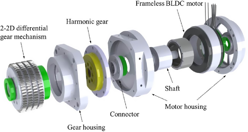
Figure 5. Details of primary driving unit.

Figure 6. Driving mechanism and flow of driving force.

Figure 7. Schematic of adhesion mechanism.

Figure 8. Calculate adhesion force.
3.3. Active adhesion mechanism
We designed the proposed robot for driving in a pipeline, including a curved pipe, a T-branch, and a miter. Specifically, the miter has a very narrow space and sharp edge because it is fabricated through piercing and welding. Thus, the robot should change in size to pass through the miter. Furthermore, when the robot moves in a vertical pipe or with additional equipment to inspect the pipeline, the robot’s traction force should be increased to obtain a comparable velocity. A slider-crank mechanism was applied to the proposed robot to generate the adhesion force and change the robot’s size.
As shown in Figs. 9 and 8, the adhesion force generated using a BLDC motor (EC-max 22, 25W, Maxon motor) is delivered to the screw via the spur gear train. When the screw rotates, the slider crank can be moved by the motion of the sliding plate, and each wheel moves simultaneously in accordance with this movement. The adhesion force can be adjusted by controlling the compression of the spring located at the connecting rod in the slider-crank mechanism. The front and rear wheels move simultaneously because they are symmetrically structured. The kinematic analysis of active adhesion mechanism can be expressed as follows:
 \begin{eqnarray}L_3^{2} & = & L_1^{2}+d^{2}-2L_{1}d{\rm{cos}}\theta_1 \end{eqnarray}
 \begin{eqnarray}\theta_1 & = & {\rm{cos}}^{-1}{\left(\frac{L_1^{2}+d^{2}-L_3^{2} }{2L_{1}d} \right)} \end{eqnarray}
 \begin{eqnarray}\frac{D}{2} & = & a + (L_1 + L_2){\rm{sin}}\theta_1 + r, \end{eqnarray}
where
 $\theta_1$
is the angle of the wheel arm, and
$\theta_1$
is the angle of the wheel arm, and
 $L_1,L_2,and\;L_3$
represent the length of the link. Further, D is the pipe’s diameter, and a and d are the distances of the slider from the center of the robot. According to Eqs. (1)–(3), the active adhesion mechanism produces the same motion for each wheel. In addition, it can calculate
$L_1,L_2,and\;L_3$
represent the length of the link. Further, D is the pipe’s diameter, and a and d are the distances of the slider from the center of the robot. According to Eqs. (1)–(3), the active adhesion mechanism produces the same motion for each wheel. In addition, it can calculate
 $\theta_1$
when the wheel makes contact with the pipe. After contact, spring compression generates the adhesion force. The adhesion force can be calculated as follows:
$\theta_1$
when the wheel makes contact with the pipe. After contact, spring compression generates the adhesion force. The adhesion force can be calculated as follows:
 \begin{eqnarray}L_1^{2} & = & d^{'2}+L_3^{'2}-2d^{'}L_3^{'}{\rm{cos}}\theta_2 \end{eqnarray}
 \begin{eqnarray}\theta_2 & = & {\rm{cos}}^{-1}{\left(\frac{d^{'2}+L_3^{'2}-L_1^{2}}{2d^{'}L_3^{'}} \right)} \end{eqnarray}
 \begin{eqnarray}L_3^{'} & = & \sqrt{L_1^2+d^{'2}-2L_{1}d^{'}{\rm{cos}}\theta_1} \end{eqnarray}
Finally, we have
 \begin{eqnarray}F & = & k(L_3-L_3^{'}) \end{eqnarray}
 \begin{eqnarray}F_n & = & F{\rm{cos}}(90^{\circ}-\theta_2) ,\end{eqnarray}
where
 $\theta_2$
is the angle of the
$\theta_2$
is the angle of the
 $L_3^{'}$
link, and
$L_3^{'}$
link, and
 $d^{'}$
and
$d^{'}$
and
 $d^{'}$
represent the changed lengths. F is the spring force, and k is a constant.
$d^{'}$
represent the changed lengths. F is the spring force, and k is a constant.
 $F_n$
represents adhesion force.
$F_n$
represents adhesion force.
3.4. Roll joint mechanism
The roll joint mechanism consists of a BLDC motor (EC-max 22, 25 W, Maxon motor), gear train, and absolute magnet encoder, as shown in Fig. 9. Because we developed a joint module with a two-pitch axis for connecting each module, having a roll joint is necessary to enable three-dimensional movements. When the direction of movement varies from the joint axis, the robot can align the axis of each joint module using the roll joint mechanism.

Figure 9. Details of roll joint mechanism.
4. Joint Module
The modularized in-pipe robot requires a joint mechanism to connect to the other modules. The joint mechanism can be classified into two types depending on the operating method: The first type is a passive joint mechanism that does not contain any actuator to control. It is typically used in robots that can control other modules using their own directions. Furthermore, this module type has a simple mechanical structure, such as a universal joint or springs. The second type, that is, the active joint mechanism not only connects the modules but also controls the joint angle for steering in the pipeline. It is more beneficial for overcoming the various pipe elements and actively selecting the direction of movement. However, the power consumption of the active joint mechanism is higher than that of the passive joint mechanism because the active joint mechanism must have an actuator for control. Thus, we propose a joint mechanism to provide active control and passive compliance of the joint module selectively based on the back-drivable mechanism, as described in Fig. 10a and Table II [Reference Martin and Grossard25].

Figure 10. Two-pitch joint mechanism.
Table II. Overall specifications of joint module.

As shown in Fig. 10b, we developed a back-drivable joint mechanism to make it suitable for MRINSPECT VII+. A previous study verified the basic operation of the back-drivable joint mechanism [Reference Kim, Yang, Choi, Mun, Park and Choi26]. The power transmission process of the joint module is expressed as follows: The gear train transfers the output torque from the motor to the ball screw. The slider connected to the ball screw translates as the ball screw rotates, and the force is amplified. At this time, the wire fixed to the slider is also translated, and the pulley of the movable plate rotates by friction with the wire. The magnetic attached to the movable plate as well as the absolute encoder attached to the main plate determine the pitch angle of the joint module. As mentioned earlier, it can be used in both passive and active modes. In passive mode, no current is applied to the BLDC motor, and the pitch angle of the joint module changes according to the force applied to the movable plate. This feature is used mainly when the modules connected to the movable plate are all in contact with the inner wall of straight pipelines or elbows, so that the pitch angle can be changed without control according to the pipe shape. In active mode, the current is applied to the BLCD motor to allow control. This characteristic is useful when the modules connected to the movable plate are not in contact with the inner wall of the pipe like the miter, and therefore requires its own force and control. The joint torque can be calculated as follows:
 \begin{equation}F_a=\frac{M_{motor} \times 2\pi \times i \times \eta _{motor} \times \eta _{gearhead} \times \eta _{ball screw}}{p}\end{equation}
 \begin{equation}\tau _{pitch joint}=F_a \times r_{active pulley}\end{equation}
Here,
 $M_{motor}$
is the nominal torque of the motor.
$M_{motor}$
is the nominal torque of the motor.
 $\eta_{motor}$
,
$\eta_{motor}$
,
 $\eta_{gearhead}$
, and
$\eta_{gearhead}$
, and
 $\eta_{ballscrew}$
represent the efficiencies of the components.
$\eta_{ballscrew}$
represent the efficiencies of the components.
 $F_{a}$
is the axial force generated from the ball screw, and
$F_{a}$
is the axial force generated from the ball screw, and
 $r_{active pulley}$
is the radius of the active pulley.
$r_{active pulley}$
is the radius of the active pulley.
The proposed robot consists of several modules, including driving, sensor, and battery modules. We connected each module through joint modules. The proposed joint module has a two-pitch axis to steer in the miter, which is the worst condition in a pipe element. Compared with a single pitch joint or universal joint, it provides a high available volume for other modules when the robot follows the center line of the pipe element. Furthermore, it can reduce the computing cost for controlling because only four or fewer pitch axes are controlled for steering. The proposed robot follows the center line of the pipeline [Reference Lee, Kim, Choi, Jang and Choi27]. Thus, we introduce each joint angle to steer in the miter. It can be divided into four stages, as shown in Fig. 10c: the first stage continues until the front module moves from the start point of the miter to the end point; the front module follows the circular path with a curvature of 0.5D, when the robot moves in the first step. The joint angles were calculated as follows:
 \begin{equation}\alpha=180^{\circ}-{\rm{cos}}^{-1}\frac{{x_1}^{2}+c^{2}-a^{2}}{2c\sqrt{(0.5D)^2+{x_1}^{2}}}-{\rm{cos}}^{-1}\frac{0.5D}{\sqrt{(0.5D)^{2}+{x_1}^{2}}}\end{equation}
 \begin{equation}\beta=270^{\circ}-{\rm{cos}}^{-1}\frac{{a}^{2}+c^{2}-{x_1}^{2}}{2c\sqrt{(0.5D)^2+{a}^{2}}}-{\rm{cos}}^{-1}\frac{a}{\sqrt{(0.5D)^{2}+{a}^{2}}}\end{equation}
The second and third steps involve the alignment processes for following the centerline by the linear motion of each module, respectively. The movements of each module were calculated as follows:
 \begin{equation}\alpha=90^{\circ}+{\rm{sin}}^{-1}\frac{|(a-0.5D)-{x_2}|}{c}\end{equation}
 \begin{equation}\beta=180^{\circ}-{\rm{sin}}^{-1}\frac{|(a-0.5D)-{x_2})|}{c}\end{equation}
 \begin{equation}\alpha=90^{\circ}+{\rm{sin}}^{-1}\frac{|(a-0.5D)-{x_3}|}{c}\end{equation}
 \begin{equation}\beta=180^{\circ}-{\rm{sin}}^{-1}\frac{|(a-0.5D)-{x_3}|}{c}\end{equation}
As explained in Fig. 10c, when the second module moves in the miter, the fourth step controls the four-pitch axis. The relationship of each joint can be calculated, as shown in Eqs. (17)–(20).
 \begin{equation}\alpha=270^{\circ}-{\rm{cos}}^{-1}\frac{{b}^{2}+c^{2}-{x_4}^{2}}{2c\sqrt{(0.5D)^2+{b}^{2}}}-{\rm{cos}}^{-1}\frac{b}{\sqrt{(0.5D)^{2}+{b}^{2}}}\end{equation}
 \begin{equation}\beta=180^{\circ}-{\rm{cos}}^{-1}\frac{{x_4}^{2}+c^{2}-{b}^{2}}{2c\sqrt{(0.5D)^2+{x_4}^{2}}}-{\rm{cos}}^{-1}\frac{0.5D}{\sqrt{(0.5D)^{2}+{x_4}^{2}}}\end{equation}
 \begin{equation}\alpha^{'}=180^{\circ}-{\rm{cos}}^{-1}\frac{{x^{'}_1}^{2}+c^{2}-b^{2}}{2c\sqrt{(0.5D)^2+{x^{'}_1}^{2}}}-{\rm{cos}}^{-1}\frac{0.5D}{\sqrt{(0.5D)^{2}+{x^{'}_1}^{2}}}\end{equation}
 \begin{equation}\beta^{'}=270^{\circ}-{\rm{cos}}^{-1}\frac{{a}^{2}+c^{2}-{x^{'}_1}^{2}}{2c\sqrt{(0.5D)^2+{b}^{2}}}-{\rm{cos}}^{-1}\frac{b}{\sqrt{(0.5D)^{2}+{b}^{2}}}\end{equation}
In these equations,
 $\alpha$
,
$\alpha$
,
 $\alpha^{'}$
,
$\alpha^{'}$
,
 $\beta$
, and
$\beta$
, and
 $\beta^{'}$
are the angles of each pitch axis, and c is the joint length. In addition,
$\beta^{'}$
are the angles of each pitch axis, and c is the joint length. In addition,
 $x_1,x_2,x_3,x_4,x_1^{'}$
, and
$x_1,x_2,x_3,x_4,x_1^{'}$
, and
 $x_4^{'}$
are the moving distances of the module, such as the sensor and driving modules. When the configuration of the robot is expanded, additional modules sequentially follow these stages.
$x_4^{'}$
are the moving distances of the module, such as the sensor and driving modules. When the configuration of the robot is expanded, additional modules sequentially follow these stages.
5. Sensor Module
The proposed robot has a sensor module implemented with PSD sensors (VL53L0X, ST) to recognize the pipe element, a CCD camera (FMVU-13S2C-CS, Point Grey) for visual inspection, an IMU sensor (3DM-GX4-25,MicroStrain Sensing Systems) to measure the robot posture, and an SBC (Intel Atom N3845 (4x 1.9GHz), Quad Core) to control the robot. Furthermore, we installed an RF antenna for wireless communication, as shown in Fig. 11a. We developed an algorithm to identify six pipe elements in a previous study [Reference Choi, Kim, Mun, Lee and Choi28]. However, the algorithm proposed in this paper can recognize eight pipe elements, and we added a method to compensate for errors caused by the deviation of the sensor module from the center point of the pipe. The sensor module discriminates the eight elements and recognizes the directions. In conjunction with the joint module angle control method described in Section 4, we also developed an autonomous driving algorithm based on sensor data.

Figure 11. Proposed sensor module and battery module.
5.1 Control architecture
Figure 12 shows the sensors the robot uses mainly to recognize the pipe environment: a PSD sensor and odometry. We attached two PSD sensors to the front of the sensor module at
 $180^{\circ}$
circumferentially, as well as eight PSD sensors to the side of the sensor module at intervals of
$180^{\circ}$
circumferentially, as well as eight PSD sensors to the side of the sensor module at intervals of
 $45^{\circ}$
. The selected sensors can measure distances from 1 mm to 1 m, as shown in Fig. 11a. We attached odometry to the passive wheels, two for each driving module. The sensor data entered the SBC in the sensor module through CAN communication. Through the inner-control software, four tasks determine the most suitable pitch angle of the joint modules in the pipeline: recognition, localization, mapping, and motion control. In addition, the operation of the driving module was determined. Recognition detects frontal pipe elements and directions, and localization calculates the current moving distance of each module based on odometry and joint angles. Mapping determines the route in 3D coordinates based on the current moving distance of the front sensor module, recognized pipe element, and direction information. Finally, the joint modules and driving modules are controlled based on the start and end points of the pipe elements.
$45^{\circ}$
. The selected sensors can measure distances from 1 mm to 1 m, as shown in Fig. 11a. We attached odometry to the passive wheels, two for each driving module. The sensor data entered the SBC in the sensor module through CAN communication. Through the inner-control software, four tasks determine the most suitable pitch angle of the joint modules in the pipeline: recognition, localization, mapping, and motion control. In addition, the operation of the driving module was determined. Recognition detects frontal pipe elements and directions, and localization calculates the current moving distance of each module based on odometry and joint angles. Mapping determines the route in 3D coordinates based on the current moving distance of the front sensor module, recognized pipe element, and direction information. Finally, the joint modules and driving modules are controlled based on the start and end points of the pipe elements.

Figure 12. Control architecture.
5.2 Recognition
Figure 13 shows the recognizable pipe elements. When inside a straight pipe, all the sensor values on the side show the same value as the pipe radius. However, the sensor value closest to the pipe direction shows a significant change in the other elements, so the influence of noise can be minimized. Figure 14 shows the recognition algorithm.
 $d_f$
is the average value of the front PSD sensors, and
$d_f$
is the average value of the front PSD sensors, and
 $d_s$
is the reading of the side PSD with a maximum value. r is the pipe radius, and e is the sum of errors caused by the sensor module leaving the center of the pipe and its own sensor error.
$d_s$
is the reading of the side PSD with a maximum value. r is the pipe radius, and e is the sum of errors caused by the sensor module leaving the center of the pipe and its own sensor error.
 $d_o$
is the moving distance based on the odometry.
$d_o$
is the moving distance based on the odometry.

Figure 13. Target pipe elements and navigation route.

Figure 14. Recognition algorithm.
First, the average value of the front PSD sensors and the largest value among the side PSD sensors can be divided into five groups, as shown in layer 1 of Fig. 14.
 $(2\sqrt{2} + 1)r$
is the front and side length of the
$(2\sqrt{2} + 1)r$
is the front and side length of the
 $45^{\circ}$
miter route 2 at the point in which the largest value among the side PSD sensors changes drastically. In the straight pipe, the side sensor values were similar to the pipe radius, and the front sensor values showed the largest value of the sensor’s measurement range. In the curved pipe, the front sensor values are smaller.
$45^{\circ}$
miter route 2 at the point in which the largest value among the side PSD sensors changes drastically. In the straight pipe, the side sensor values were similar to the pipe radius, and the front sensor values showed the largest value of the sensor’s measurement range. In the curved pipe, the front sensor values are smaller.
Next, the elements of the first group – miter route 1, T-branch route 1, and
 $45^{\circ}$
miter route 1 – can be classified. A simulation performed based on the point of entry into the element determined the boundary condition, as shown in Fig. 15. With the sensors attached at
$45^{\circ}$
miter route 1 – can be classified. A simulation performed based on the point of entry into the element determined the boundary condition, as shown in Fig. 15. With the sensors attached at
 $45^{\circ}$
intervals, the pipe direction will be within
$45^{\circ}$
intervals, the pipe direction will be within
 $\pm 22.5^{\circ}$
relative to the side PSD sensor angle, which has the largest value. In addition, because all elements are symmetrical to the pipe direction, the plus and minus signs do not affect the side PSD sensor data. Therefore, we simulated two cases of
$\pm 22.5^{\circ}$
relative to the side PSD sensor angle, which has the largest value. In addition, because all elements are symmetrical to the pipe direction, the plus and minus signs do not affect the side PSD sensor data. Therefore, we simulated two cases of
 $0^{\circ}$
and
$0^{\circ}$
and
 $22.5^{\circ}$
based on the pipe direction of each pipe element. Theoretically, the largest PSD sensor value exists between these two graphs, regardless of the pipe direction angle.
$22.5^{\circ}$
based on the pipe direction of each pipe element. Theoretically, the largest PSD sensor value exists between these two graphs, regardless of the pipe direction angle.
The simulation results show that the slope of the largest side PSD data in the miter decreases after entering the element, whereas in the T-branch, the slope increases gradually. The
 $45^{\circ}$
miter exhibits a constant slope. Based on this simulation data, we developed an algorithm that distinguishes the first group using the slope, largest side PSD value, and odometry value, as shown in Fig. 14 Layer 2. In miter route 2 and T-branch route 2, the same threshold is applied because the largest side sensor data changes identically.
$45^{\circ}$
miter exhibits a constant slope. Based on this simulation data, we developed an algorithm that distinguishes the first group using the slope, largest side PSD value, and odometry value, as shown in Fig. 14 Layer 2. In miter route 2 and T-branch route 2, the same threshold is applied because the largest side sensor data changes identically.

Figure 15. Simulation results of largest side PSD data and moving distance in pipe elements.
Next, detecting the direction of each distinguished pipe element is necessary for proper routing, as shown in Fig. 16. To obtain the direction of the elbow, we used from the sum of the eight side PSD sensor values inside the elbow pipe, as shown in Fig. 16a. However, the error caused by the deflection of the sensor module from the center of the pipe can be reduced by subtracting the sum of the side PSD sensor values before entering the curved pipe. Each sensor has a fixed angle,
 $\theta_i$
, based on the robot coordinates, and the direction can be obtained as follows:
$\theta_i$
, based on the robot coordinates, and the direction can be obtained as follows:
 \begin{equation}\theta_{hole} = {\rm{atan2}}\left(\sum_{i=1}^{8}l_{bi}{\rm{sin}}\theta_i-l_{ai}{\rm{sin}}\theta_i,\sum_{i=1}^{8}l_{bi}{\rm{cos}}\theta_i-l_{ai}{\rm{cos}}\theta_i\right)\end{equation}

Figure 16. Principles of sensing direction.
The inner cross-section of the
 $45^{\circ}$
miter forms an elliptical and circular overlapping shape. In route 1, the distance between the center of the ellipse and circle d gradually increases as the sensor module enters (refer to Fig. 16b). On the contrary, in route 2, the distance becomes shorter. The formula for determining the direction is as follows:
$45^{\circ}$
miter forms an elliptical and circular overlapping shape. In route 1, the distance between the center of the ellipse and circle d gradually increases as the sensor module enters (refer to Fig. 16b). On the contrary, in route 2, the distance becomes shorter. The formula for determining the direction is as follows:
 \begin{equation}F(x,y,\theta)=\frac{{({x{\rm{cos}}}\theta+y{\rm{sin}}\theta-d)}^2}{2r^{2}}+\frac{{({-x{\rm{sin}}}\theta+y{\rm{cos}}\theta)}^2}{r^{2}}=1\end{equation}
 \begin{equation}F(x_i,y_i,\theta_{hole})-F(x_{i-1},y_{i-1},\theta_{hole})=0\end{equation}
 \begin{equation}d(i)=\frac{2(l_i^2-l_{i-1}^2)-{(x_i{\rm{cos}}\theta_{hole}+{y_i{\rm{sin}}\theta_{hole}})}^2+{(x_{i-1}{\rm{cos}}\theta_{hole}+{y_{i-1}{\rm{sin}}\theta_{hole}})}^2}{2(x_i{\rm{cos}}\theta_{hole}+{y_i{\rm{sin}}\theta_{hole}}-x_{i-1}{\rm{cos}}\theta_{hole}-{y_{i-1}{\rm{sin}}\theta_{hole}})}\end{equation}
 $l_i$
is the largest distance sensor value (refer to Fig. 16b), and
$l_i$
is the largest distance sensor value (refer to Fig. 16b), and
 $\theta_i$
is the fixed angle of the PSD sensor based on the robot coordinates.
$\theta_i$
is the fixed angle of the PSD sensor based on the robot coordinates.
 $x_i = l_i{\rm{cos}}\theta_i$
is the x coordinate of the point that
$x_i = l_i{\rm{cos}}\theta_i$
is the x coordinate of the point that
 $i_{th}$
sensor detects, and
$i_{th}$
sensor detects, and
 $y_i = l_i{\rm{sin}}\theta_i$
is the y coordinate of the point. Eq. (22) is the general solution of the ellipse in terms of robot coordinates, r is the pipe radius, and
$y_i = l_i{\rm{sin}}\theta_i$
is the y coordinate of the point. Eq. (22) is the general solution of the ellipse in terms of robot coordinates, r is the pipe radius, and
 $\theta$
is the pipe direction. Because the
$\theta$
is the pipe direction. Because the
 $(i-1)_{th}$
PSD also detects the same ellipses, substituting them into the elliptic equation and calculating like Eq. (23) can be summed up in terms of d, as shown in Eq. (24). In this equation, the unknowns are
$(i-1)_{th}$
PSD also detects the same ellipses, substituting them into the elliptic equation and calculating like Eq. (23) can be summed up in terms of d, as shown in Eq. (24). In this equation, the unknowns are
 $\theta_{hole}$
and d, and the
$\theta_{hole}$
and d, and the
 $(i + 1)_{th}$
PSD also detects the same ellipse. Thus, when d(i) and
$(i + 1)_{th}$
PSD also detects the same ellipse. Thus, when d(i) and
 $d(i+1)$
values are the same,
$d(i+1)$
values are the same,
 $\theta_{hole}$
is the direction of the
$\theta_{hole}$
is the direction of the
 $45^{\circ}$
miter.
$45^{\circ}$
miter.
T-branch route 1 and miter route 1 show the same cross section when the side PSD sensors detect the inside of the lateral pipe; thus, the direction can be estimated in the same way (refer to Fig. 16c). The formula used to determine the direction is as follows:
 \begin{equation}\theta_{hole} = {\rm{atan2}}(l_{i+1}{\rm{sin}}\theta_{i+1}+l_{i-1}{\rm{sin}}\theta_{i-1}+2l_{c}{\rm{sin}}\theta_{c}, l_{i+1}{\rm{cos}}\theta_{i+1}+l_{i-1}{\rm{cos}}\theta_{i-1}+2l_{c}{\rm{cos}}\theta_{c})\end{equation}
 \begin{equation}\theta_{c1} ={\rm{acos}}(\frac{\sqrt{{(l_{i+3}{\rm{sin}}\theta_{i+3}-l_{i-3}{\rm{sin}}\theta_{i-3})}^2+{(l_{i+3}{\rm{cos}}\theta_{i+3}-l_{i-3}{\rm{cos}}\theta_{i-3})}^2}}{2r})\end{equation}
 \begin{equation}\theta_{c2} ={\rm{atan2}}(l_{i+3}{\rm{sin}}\theta_{i+3}-l_{i-3}{\rm{sin}}\theta_{i-3}, l_{i+3}{\rm{cos}}\theta_{i+3}-l_{i-3}{\rm{cos}}\theta_{i-3})\end{equation}
 \begin{equation}\theta_{c} = \theta_{c1} +\theta_{c2} -180^{\circ}\end{equation}
 \begin{equation}l_{c} = \sqrt{{(l_{i-3}{\rm{sin}}\theta_{i-3}+r{\rm{sin}}\theta_{c})}^2+{(l_{i-3}{\rm{cos}}\theta_{i-3}+r{\rm{cos}}\theta_{c})}^2}\end{equation}
Assuming that the
 $i_{th}$
PSD is the side PSD sensor with the largest value, the pipe direction can be obtained as the vector sum of the
$i_{th}$
PSD is the side PSD sensor with the largest value, the pipe direction can be obtained as the vector sum of the
 $(i+1)_{th}$
and the
$(i+1)_{th}$
and the
 $(i-1)_{th}$
PSD value. However, when the sensor module is outside the center of the pipe, an error occurs. This error can be canceled out, as shown in Eq. (25).
$(i-1)_{th}$
PSD value. However, when the sensor module is outside the center of the pipe, an error occurs. This error can be canceled out, as shown in Eq. (25).
 $l_c$
can be determined with Eqs. (26)–(29) using the data
$l_c$
can be determined with Eqs. (26)–(29) using the data
 $l_{i+3}$
,
$l_{i+3}$
,
 $l_{i-3}$
, and the pipe radius.
$l_{i-3}$
, and the pipe radius.
Because T-branch route 2 and miter route 2 have the same cross-sectional shape inside the pipe element, we can estimate the pipe direction in the same way as shown in Fig. 16d). The formula used to determine the direction is as follows:
 \begin{equation}x_{a}=l_{i+1}{\rm{cos}}\theta_{i+1}+l_{i-1}{\rm{cos}}\theta_{i-1}, \> y_{a}=l_{i+1}{\rm{sin}}\theta_{i+1}+l_{i-1}{\rm{sin}}\theta_{i-1}\end{equation}
 \begin{equation}x_{b}=l_{i+3}{\rm{cos}}\theta_{i+3}+l_{i-3}{\rm{cos}}\theta_{i-3}, \> y_{b}=l_{i+3}{\rm{sin}}\theta_{i+3}+l_{i-3}{\rm{sin}}\theta_{i-3}\end{equation}
 \begin{equation}\theta_{hole1} = {\rm{atan2}}(y_{b}-y_{a},x_{b}-x_{a}), \> \theta_{hole2} = {\rm{atan2}}(y_{a}-y_{b},x_{a}-x_{b})\end{equation}
Assuming that
 $i_{th}$
PSD is the side PSD sensor with the largest value, the pipe direction can be obtained from the vector sum of
$i_{th}$
PSD is the side PSD sensor with the largest value, the pipe direction can be obtained from the vector sum of
 $(i+1)_{th}$
and
$(i+1)_{th}$
and
 $(i-1)_{th}$
and the vector sum of
$(i-1)_{th}$
and the vector sum of
 $(i+3)_{th}$
and
$(i+3)_{th}$
and
 $(i-3)_{th}$
based on the robot coordinate system. However, an error occurs when the sensor module is outside the center of the pipe. Route 2 has two pipe holes that are
$(i-3)_{th}$
based on the robot coordinate system. However, an error occurs when the sensor module is outside the center of the pipe. Route 2 has two pipe holes that are
 $180^{\circ}$
apart in the direction of (
$180^{\circ}$
apart in the direction of (
 $\theta_{hole1}$
and
$\theta_{hole1}$
and
 $\theta_{hole2}$
), so the error can be canceled out using Eqs. (30)–(32).
$\theta_{hole2}$
), so the error can be canceled out using Eqs. (30)–(32).
5.3 Localization and mapping
For control and inspection, knowing the external environment and the location of the robot in motion is necessary. Figure 17 shows the calculation of the travel distance of each module based on the odometry data. Each module is numbered sequentially from the front, based on the travel direction of travel. When the module receiving the odometry data is the
 $n_{th}$
module, as shown in Fig. 17a, the moving distance of each module center(
$n_{th}$
module, as shown in Fig. 17a, the moving distance of each module center(
 $d_i$
) can be calculated by the method suggested in Fig. 17b. The formula for calculating
$d_i$
) can be calculated by the method suggested in Fig. 17b. The formula for calculating
 $d_i$
in a straight pipe is as follows:
$d_i$
in a straight pipe is as follows:
 \begin{equation}d_{i}=\begin{cases} d_{i+1}+l_{b(i)} & (i<n) \\ d_i = d_o & (i=n) \\ d_{i-1}-l_{b(i)} & (i>n) \end{cases}\end{equation}
 $l_{b(i)}$
is the distance between the center of the
$l_{b(i)}$
is the distance between the center of the
 $i_{th}$
module and the center of the
$i_{th}$
module and the center of the
 $i+1_{th}$
module.
$i+1_{th}$
module.
 $d_o$
is the odometry-based moving distance.
$d_o$
is the odometry-based moving distance.

Figure 17. Principle of real time localization.
Figure 18 shows how to store map information when an element is recognized. i is the number of pipe elements changed, and
 $t_i$
is the integer number of
$t_i$
is the integer number of
 $i_{th}$
pipe type (e.g., straight = 1).
$i_{th}$
pipe type (e.g., straight = 1).
 $\theta_i$
is the direction of the
$\theta_i$
is the direction of the
 $i_{th}$
pipe, and
$i_{th}$
pipe, and
 $p_i$
is the starting point of the
$p_i$
is the starting point of the
 $i_{th}$
pipe. As shown in Figs. 18a and 18b, initialization occurs at the start of driving; when a different pipe is recognized, a path is set according to the pipe type. Here,
$i_{th}$
pipe. As shown in Figs. 18a and 18b, initialization occurs at the start of driving; when a different pipe is recognized, a path is set according to the pipe type. Here,
 $l_c$
is the entry distance when recognized, and
$l_c$
is the entry distance when recognized, and
 $l_d$
is the path distance according to the pipe type. The pipe information is updated whenever the pipe type recognized just before entering and the newly recognized pipe type are different according to the recognition algorithm. Figure 19 shows the driving route inside the elbow.
$l_d$
is the path distance according to the pipe type. The pipe information is updated whenever the pipe type recognized just before entering and the newly recognized pipe type are different according to the recognition algorithm. Figure 19 shows the driving route inside the elbow.
 $\theta$
is the rolling angle of the elbow, and d is the moving distance inside the elbow.
$\theta$
is the rolling angle of the elbow, and d is the moving distance inside the elbow.
 $l_R$
represents the radius of curvature, whereas
$l_R$
represents the radius of curvature, whereas
 $\varphi$
represents the moving angle along d. In this case, the 4-by-4 transformation matrix equation is as follows:
$\varphi$
represents the moving angle along d. In this case, the 4-by-4 transformation matrix equation is as follows:
 \begin{equation}^B_A\mathbf{T}= \begin{bmatrix} {\rm{cos}}\theta\;\;\;\; & -{\rm{sin}}\theta\;\;\;\; & 0\;\;\;\; & 0 \\ {\rm{sin}}\theta\;\;\;\; & {\rm{cos}}\theta\;\;\;\; & 0\;\;\;\; & 0 \\ 0\;\;\;\; & 0\;\;\;\; & 1\;\;\;\; & 0 \\ 0\;\;\;\; & 0\;\;\;\; & 0\;\;\;\; & 1 \end{bmatrix}\begin{bmatrix} 1\;\;\;\; & 0\;\;\;\; & 0\;\;\;\; & l_R(1-{\rm{cos}}\varphi) \\ 0\;\;\;\; & 1\;\;\;\; & 0\;\;\;\; & 0 \\ 0\;\;\;\; & 0\;\;\;\; & 1\;\;\;\; & l_R({\rm{sin}}\varphi) \\ 0\;\;\;\; & 0\;\;\;\; & 0\;\;\;\; & 1 \end{bmatrix}\begin{bmatrix} {\rm{cos}}(-\varphi)\;\;\;\; & 0\;\;\;\; & {\rm{sin}}(-\varphi)\;\;\;\; & 0 \\ 0\;\;\;\; & 1\;\;\;\; & 0\;\;\;\; & 0 \\ -{\rm{sin}}(-\varphi)\;\;\;\; & 0\;\;\;\; & {\rm{cos}}(-\varphi)\;\;\;\; & 0 \\ 0\;\;\;\; & 0\;\;\;\; & 0\;\;\;\; & 1 \end{bmatrix}\end{equation}
Accordingly, by knowing the moving distance and direction of the recognized pipe element, we can know the location of the robot with three-dimensional coordinates. In addition, we standardized other pipe elements that require steering of the robot so that we can estimate the three-dimensional coordinates of the robot when the curvature is substituted into the above equation according to the pipe type (see Table III). In addition,
 $l_D$
in Fig. 18 is derived from the bending angle according to the pipe type.
$l_D$
in Fig. 18 is derived from the bending angle according to the pipe type.
Table III. Trajectry parameters of pipe elements.


Figure 18. Principle of map information storage.

Figure 19. Trajectry in elbow.
Pipe elements that do not require steering can be updated by multiplying the z-axis translation matrix. By multiplying some transformation matrix sequentially according to the stored map information, we can determine the current robot position, as shown in Fig. 20a, even if it passes through several pipe elements. Finally, we developed software that uses the location and information of the pipe elements to provide a graphical three-dimensional map, as shown in Fig. 20b.

Figure 20. 3D-position calculation and map.
6. Battery Module
The battery module was designed using lithium-ion batteries, as shown in Fig. 11b. This lithium-ion battery pack has a 7S7P configuration with 25.4 V, 24.5 Ah capacity, and 70 A maximum continuous discharge rating. We installed a battery based on the maximum available volume to maximize the battery capacity.
7. Wireless Communication
In terms of cost, wireless communication is more advantageous than wired communication when a robot travels a long distance. In wired communication, the longer the robot travels, the longer is the length of the cable. In this case, the traction force of the robot must also be larger, and equipment, such as a cable winch that supports during operation, also grows.
MRINSPECT VII + has been developed for long-distance inspection and has adopted wireless communication, as shown in Fig. 21. Communication is performed through the following process: First, the user of the operating station uses the control PC to make a wireless connection to the ethernet repeater. The repeater transmits signals to the antenna installed in the piping through the UTP cable, and the antenna enables long-distance wireless communication within the pipe. The RF module mounted on the sensor module of the robot receives this signal. This process finally enables communication between the user in the operating station and the robot inside the pipe. The user confirms the robot’s position and controls it through this communication. In addition, visual inspection is carried out through the CCD camera attached to the sensor module, the data of the inspection tool is received, and defects of the pipe are detected in real time.

Figure 21. Configuration of wireless communication between the operator and the robot.
8. Experiments
8.1 Experimental setup
As shown in Fig. 22, the primary PC displays the current state of the robot as well as the inside view from the CCD camera. In addition, wireless communication transfers the desired command to the SBC. The SBC calculates the driving algorithm and transfers the desired velocity and angle to each control board installed in the driving module. It communicates through CAN communication to each motor driver (EPOS4 Module 50/8, MAXON motor) and the SBC designed from the control board using ARM(STM32F1, ST).

Figure 22. Schematic diagram of robot system.
8.2 Single module experiment
Before running the experiment with the fully assembled robot, we proved the performance of each module, the single driving module, and the joint module. The driving experiment was performed using a single driving module, and it can drive in curved and vertical pipes, as shown in Figs. 23a and 23b, respectively. In addition, we used a push–pull gauge (RX-20, AIKOH) to test the traction force of the driving module in a steel pipe. The maximum force of the driving module is 166.3 N.

Figure 23. Single module driving experimental results.
8.3 Multiple module experiment
We used an extended robot with additional inspection modules to perform driving experiments of several pipe elements. The robot can pass through a curved pipe, miter, and vertical pipe without colliding with the acrylic pipe element, as shown in Figs. 24a to 24c. When the robot moved in a curved pipe, the joint modules without the first and last joint modules, which were connected to the sensor modules, were passive modes. When the robot overcame the miter, every joint in the proposed stage was controlled to follow the calculated path. In addition, we combined the recognition algorithm of the pipe element and the driving algorithm for autonomous driving. As a result, in the steel pipe element, the robot can autonomously drive through curved pipes and miters without collision, as shown in Figs. 24d and 24e, respectively.

Figure 24. Multi module driving experiment results.
8.4 Long-range driving experiment
A long-distance driving test was conducted using a battery. As shown in Fig. 25a, we used a 30-m steel pipe to build an experimental environment. We verified the maximum driving distance through continuous repeated driving in the pipe. The maximum distance was 760 m within 2 and 14 min. The maximum velocity was 120 mm/s, and the average velocity was 94 mm/s. Figure 25b shows the distance information from the odometer, which was attached to the driving module.

Figure 25. Results of long-range driving experiment.
8.5 Outdoor experiment
A high-pressure resistance test was conducted in the PSF, which is a simulation pipeline network located at KOGAS (Korea Gas Corporation). As shown in Fig. 26a, after applying the robot to the launcher of the PSF, the pressure inside the pipe of the PSF was set to 50 bar by filling it with nitrogen. The robot could withstand a total of 3 h at 50 bar. Following the high-pressure resistance test, all modules of the robot system still operated well, meaning that the proposed robot system can perform proper pipe inspection in such a pressured environment. In addition, the robot inspected the outdoor pipe, as shown in Fig. 26b

Figure 26. Outdoor experiment.
9. Conclusions
We presented MRINSPECT VII+, the newest pipe inspection robot. It has a modularized design so that the robot configuration can be easily changed. Each module was developed for a specific function. This paper explains the design, manufacturing, and improvements over the previous robot. The proposed robot can drive inside pipe elements while carrying inspection tools. We proved the robot’s performance through several experiments. In particular, through an autonomous driving experiment and a high-pressure resistance experiment, we proved the robot’s capability to inspect pipelines in real situations.
Author Contributions
Heesik Jang and Min Sub Lee developed a control algorithm. Ho Moon Kim and Yoon Geon Lee designed the mechanisms and electrical equipment. Yong Heon Song conducted the experiments. Whee Ryeong Ryew and Hyouk Ryeol Choi conceived and designed the study.
Financial Support
This work was supported by the National Research Foundation of Korea (NRF) grant funded by the Korea government (MSIT) (No. 2021R1A2C3012387).
Competing Interests Declaration
The authors declare none.


