


1. Introduction
Driven by numerous applications of polydispersed multiphase flow, e.g. the rain formation in atmospheric cloud turbulence or the mist of droplets in the combustion chamber of automobile or aeronautic engines, an abundant number of experimental, numerical and theoretical studies on inertial particles in turbulence can be found in the literature (see, e.g. Shaw Reference Shaw2003; Toschi & Bodenschatz Reference Toschi and Bodenschatz2009; Elghobashi Reference Elghobashi2019).
Self-organisation of the particle density into cluster and void regions is hereby a typical feature observed in particle-laden turbulent flows and understanding the dynamics is critical for the required mathematical modelling. The divergence of the particle velocity, which differs due to inertial effects from the divergence-free fluid velocity, plays a crucial role for this clustering mechanism.
Early results for clustering in particle-laden turbulent flows have been presented in Eaton & Fessler (Reference Eaton and Fessler1994), and further progress of understanding clustering in homogeneous isotropic turbulence was well summarised in Monchaux, Bourgoin & Cartellier (Reference Monchaux, Bourgoin and Cartellier2012). The relationship between the divergence of inertial particle velocity and the background flow field was derived by Robinson (Reference Robinson1956) and Maxey (Reference Maxey1987). They showed that the divergence is proportional to the second invariant of flow velocity gradient tensor for sufficiently small Stokes numbers, which is defined as the ratio of the particle relaxation time  $\tau _p$ to the Kolmogorov time
  $\tau _\eta$. This relationship implies that particles tend to concentrate in low vorticity and high strain rate regions in turbulence. This is referred to as the preferential concentration mechanism. Many theoretical analyses of the preferential concentration have been established following Maxey's approach (e.g. Elperin, Kleeorin & Rogachevskii Reference Elperin, Kleeorin and Rogachevskii1996; Elperin et al. Reference Elperin, Kleeorin, L'vov, Rogachevskii and Sokoloff2002; Chun et al. Reference Chun, Koch, Rani, Ahluwalia and Collins2005; Esmaily-Moghadam & Mani Reference Esmaily-Moghadam and Mani2016). To understand clustering for large Stokes numbers, Vassilicos’ group (Chen, Goto & Vassilicos Reference Chen, Goto and Vassilicos2006; Goto & Vassilicos Reference Goto and Vassilicos2006, Reference Goto and Vassilicos2008; Coleman & Vassilicos Reference Coleman and Vassilicos2009) proposed the sweep-stick mechanism, in which particles are swept by large-scale flow motion while sticking to clusters of stagnation points of Lagrangian fluid acceleration. This mechanism also explains the multiscale self-similar structure of inertial particle clustering. Bragg, Ireland & Collins (Reference Bragg, Ireland and Collins2015) and Ariki et al. (Reference Ariki, Yoshida, Matsuda and Yoshimatsu2018) reported that the self-similar structure of inertial particle clustering is predicted by theoretical analyses for the inertial range of turbulence, applying Maxey's formula to a coarse grained flow field at scales where the turbulence time scale is sufficiently larger than the particle relaxation time
  $\tau _p$. Being apart from the limitation of Maxey's formula, the statistical model for inertial dynamics of small heavy particles were proposed by Gustavsson & Mehlig (Reference Gustavsson and Mehlig2016). In the model the divergence was obtained from spatial Lyapunov exponents of particle dynamics considering correlation time of particle motion and flow velocity fluctuation (Gustavsson & Mehlig Reference Gustavsson and Mehlig2011; Gustavsson, Vajedi & Mehlig Reference Gustavsson, Vajedi and Mehlig2014; Gustavsson & Mehlig Reference Gustavsson and Mehlig2016). Interesting findings are that ergodic multiplicative amplification can contribute to clustering significantly under the condition of rapid turbulent velocity fluctuation.
To confirm the reliability of these mechanisms, it is important to quantify the divergence of particle velocity based on direct numerical simulation (DNS) data. Blobs of particles were proposed by Bec et al. (Reference Bec, Biferale, Cencini, Lanotte, Musacchio and Toschi2007) to define a scale-dependent volume contraction rate using Maxey's formula to determine the divergence of the particle velocity for studying coarse grained inertial particle density in the inertial range of turbulence. Esmaily-Moghadam & Mani (Reference Esmaily-Moghadam and Mani2016) have evaluated the contraction rate using DNS results to verify their theoretical analysis, but they estimated the contraction rate based on the Lagrangian velocity gradient along the trajectory of a single particle. In this paper we aim to compute the divergence directly from the position and velocity of a huge number of particles, using the Voronoi tessellation technique.
Voronoi tessellation techniques have been first applied to inertial particle clustering in a turbulent flow by Monchaux, Bourgoin & Cartellier (Reference Monchaux, Bourgoin and Cartellier2010). Tagawa et al. (Reference Tagawa, Mercado, Prakash, Calzavarini, Sun and Lohse2012) used the three-dimensional (3-D) technique to quantify the clustering of inertial particles and bubbles in homogeneous isotropic turbulence obtained by DNS. Voronoi tessellation is further applied to experimental data (Obligado et al. Reference Obligado, Teitelbaum, Cartellier, Mininni and Bourgoin2014; Sumbekova et al. Reference Sumbekova, Cartellier, Aliseda and Bourgoin2017; Petersen, Baker & Coletti Reference Petersen, Baker and Coletti2019) and numerical data (Dejoan & Monchaux Reference Dejoan and Monchaux2013; Baker et al. Reference Baker, Frankel, Mani and Coletti2017) to obtain Lagrangian statistics. The influence of Stokes and Reynolds numbers has been analysed in Sumbekova et al. (Reference Sumbekova, Cartellier, Aliseda and Bourgoin2017). Recently, local cluster analysis of small, settling, inertial particles in isotropic turbulence was performed in Momenifar & Bragg (Reference Momenifar and Bragg2020) using 3-D Voronoi tessellation.
An inherent difficulty for determining the divergence of the particle velocity is its discrete nature, i.e. it is only defined at particle positions. To this end, we propose in the present study a model for quantifying the divergence using tessellation of the particle positions. The corresponding time change of the volume is shown to yield a measure of the particle velocity divergence. Considering high-Reynolds-number DNS flow data of inertial particles in homogeneous isotropic turbulence, we determine the divergence of the particle velocity and analyse its role for structure formation.
The outline of the manuscript is as follows. In § 2 we summarise the DNS data we analyse and in § 3 the proposed approach to quantify the divergence of the particle velocity is introduced. Numerical results are presented in § 4. Finally, conclusions are drawn in § 5. Appendices A and B yield information on the reliability and the robustness of the divergence computation and a theoretical prediction of the probability distribution function (PDF) of the divergence for randomly distributed particles.
2. Direct numerical simulation data
We analyse particle position and velocity data obtained by 3-D DNS of particle-laden homogeneous isotropic turbulence presented in Matsuda et al. (Reference Matsuda, Onishi, Hirahara, Kurose, Takahashi and Komori2014). The DNS was performed for a cubic computational domain with a side length of  $2{\rm \pi}$. The incompressible Navier–Stokes equation was solved using a fourth-order finite-difference scheme. Statistically steady turbulence was obtained by forcing at large scales, i.e. for
  $k < 2.5$, where
  $k$ is the wavenumber. Discrete particles were tracked in the Lagrangian framework. The equation of particle motion is given by
 \begin{equation} d_t {\boldsymbol v_p}_j = - \frac{{\boldsymbol v_p}_j - {\boldsymbol u_p}_j}{\tau_p} , \end{equation}
where  ${\boldsymbol v_p}_j$ is the particle velocity vector and
  ${\boldsymbol u_p}_j$ is the fluid velocity vector at particle position
  ${\boldsymbol x_p}_j$. Note that subscript
  $p$ denotes the quantity at the position of a particle (e.g.
  ${\boldsymbol u_p}_j \equiv {\boldsymbol u}({\boldsymbol x_p}_j)$), and the subscript
  $j$ denotes the particle identification number (
 $\,j=1,\ldots ,N$, where
  $N$ is the total number of particles). The Stokes drag was assumed for the drag force. The relaxation time
  $\tau _p$ is independent of the particle Reynolds number. See Onishi, Baba & Takahashi (Reference Onishi, Baba and Takahashi2011), Matsuda et al. (Reference Matsuda, Onishi, Hirahara, Kurose, Takahashi and Komori2014) and Matsuda & Onishi (Reference Matsuda and Onishi2019) for details on the computational method.
The number of grid points for the flow field is  $N_g^{3} = 512^{3}$. The kinematic viscosity is
  $\nu =1.10\times 10^{-3}$. The r.m.s. of velocity fluctuation
  $u'$, energy dissipation rate
  $\epsilon$ and Taylor-microscale-based Reynolds number
  $Re_\lambda$ (
 $\equiv u' \lambda /\nu$, where
  $\lambda$ is the Taylor microscale) of obtained turbulence were
  $u'=1.01$,
  $\epsilon =0.344$ and
  $Re_\lambda = 204$. Note that Matsuda et al. (Reference Matsuda, Onishi, Hirahara, Kurose, Takahashi and Komori2014) confirmed that
  $Re_\lambda = 204$ is large enough to be representative of high-Reynolds-number turbulence at
  $k\eta > 0.05$, where
  $\eta \equiv \nu ^{3/4} \epsilon ^{-1/4}$ is the Kolmogorov scale (i.e.
  $\eta =7.90\times 10^{-3}$). It should be also noted that the number of grid points is sufficiently large for resolving the turbulent flow so that
  $k_{max} \eta$ reached 2.03, where
  $k_{max} \equiv N_g/2$. The number of particles
  $N$ is
  $1.5 \times 10^{7}$ and the Stokes number
  $St$ (
 $\equiv \tau _p/\tau _\eta$, where
  $\tau _\eta \equiv \nu ^{1/2}\epsilon ^{-1/2}$) is
  $St = 0.05$, 0.1, 0.2, 0.5, 1, 2 and 5. Particles with different Stokes numbers were tracked in an identical turbulent flow. After the turbulent flow had reached a statistically steady state, particles were randomly seeded satisfying a Poisson distribution. Effects of the reaction of particle motion to fluid flow and the interactions between particles were neglected because these effects are typically small in the time scale of
  $\tau _\eta$ for sufficiently dilute particles such as cloud droplets in atmospheric turbulence (Matsuda & Onishi Reference Matsuda and Onishi2019). In the DNS data the particle number in a volume of
  $\eta ^{3}$ is about 0.03 and close to the conditions in atmospheric clouds. For such particle densities, the point-particle approximation and the one-way coupling are justified for most of the particles. For this study, we additionally consider data of randomly distributed particles with fluid velocity at the particle positions. These data are analysed as the fluid particle case; i.e.
  $St=0$. Note that all statistical results are averaged over 10 snapshots at time
  $21 T_0 \le t \le 30 T_0$, where
  $T_0 \approx L_0/u'$ and
  $L_0$ is the representative length which gives the domain length of
  $2{\rm \pi} L_0$ (i.e.
  $L_0=1$).
Figure 1 shows two-dimensional (2-D) cuts of the particle number density for different Stokes numbers. We can clearly observe void areas for  $St=1$. For
  $St < 1$, the void areas are less clear. For
  $St > 1$, they are larger but less pronounced than for
  $St=1$.

Figure 1. Spatial distribution of the particles coloured with the divergence  $\mathcal {D}_p$ for (a)
  $St=0.05$, (b) 0.2, (c) 1 and (d) 5 at time
  $t = 24 T_0$ for a slice of thickness
  $4\eta$.
3. Voronoi tessellation to compute the particle velocity divergence
To understand the dynamics of inertial particles, in particular the clustering, we consider the particle density  $n$ in the continuous setting, as shown in many studies (e.g. Maxey Reference Maxey1987). It satisfies the conservation equation which can be written with the Lagrangian derivative,
  $D_t = \partial _t + {\boldsymbol v}\boldsymbol {\cdot } \boldsymbol {\nabla }$, as
 \begin{equation} D_t n = -n \boldsymbol{\nabla} \boldsymbol{\cdot} {\boldsymbol v}. \end{equation}
 This illustrates that we need to know the divergence of the particle velocity, which is a source term on the right-hand side of (3.1). The problem to determine  $\boldsymbol {\nabla } \boldsymbol {\cdot } {\boldsymbol v}$ is that we only know the discrete particle distribution, and, hence, we only know the particle velocity at the particle positions, i.e.
  ${\boldsymbol v_p}_j = {\boldsymbol v}({\boldsymbol x_p}_j)$, but not anywhere else. In this study we apply the Voronoi tessellation to overcome this problem.
The Voronoi tessellation (or diagram) is a technique to construct a decomposition of the space, i.e. the fluid domain, into a finite number of Voronoi cells  $C_i$. When a finite number of particles
  $p_i$ are dispersed in space, a Voronoi cell
  $C_i$ is defined as a region closer to a particle than other particles. The volume of a Voronoi cell is referred to as Voronoi volume and denoted by
  $V_{p_i}$. The cell
  $C_i$ can be interpreted as the zone of influence of the particle
  $p_i$. The larger the number of particles in a given volume, the smaller the Voronoi volume. The diagram will allow us to identify particles inside clusters (corresponding to small cells) and particles inside void regions (corresponding to large cells). A survey on Voronoi diagrams, a classical technique in computational geometry, can be found in Aurenhammer (Reference Aurenhammer1991).
We apply 3-D Voronoi tessellation to the DNS data using the Quickhull algorithm provided by the Qhull library in python (Barber, Dobkin & Huhdanpaa Reference Barber, Dobkin and Huhdanpaa1996), which has a computational complexity of  $O(N \log (N))$.
Here we propose a method to compute the divergence of the particle velocity  ${\mathcal {D}}\equiv \boldsymbol {\nabla } \boldsymbol {\cdot } {\boldsymbol v}$ in a discrete manner. Dividing (3.1) by the particle density
  $n$, we obtain
 \begin{equation} {\mathcal{D}} = -\frac{1}{n} D_t n. \end{equation}
 To calculate the Lagrangian derivative of  $n$, we define the local number density
  $n_p$ as the number density averaged over a Voronoi cell, which is given by the inverse of the Voronoi volume
  $V_p$; i.e.
  $n_p = 1/V_p$. We consider two time instances,
  $t^{k}$ and
  $t^{k+1} = t^{k} + {\rm \Delta} t$, where
  ${\rm \Delta} t$ is the time step and the superscript
  $k$ denotes the discrete time index.
The time-averaged number density change in the period of  ${\rm \Delta} t$ is given by
  $\overline {D_t n}^{{\rm \Delta} t} = (n_p^{k+1}-n_p^{k})/{\rm \Delta} t$, where
  $\bar {n}^{{\rm \Delta} t} = (n_p^{k+1}+n_p^{k})/2 + O({\rm \Delta} t)$. Thus, we obtain a finite-time discrete divergence of the particle velocity in the period of
  ${\rm \Delta} t$:
 \begin{equation} {\mathcal{D}}_p = -\frac{2}{{\rm \Delta} t} \frac{n^{k+1}_p-n^{k}_p}{n^{k+1}_p+n^{k}_p} + O({\rm \Delta} t) = \frac{2}{{\rm \Delta} t} \frac{V^{k+1}_p-V^{k}_p}{V^{k+1}_p+V^{k}_p} + O({\rm \Delta} t) \end{equation}
which depends on the choice of  ${\rm \Delta} t$ and
  $N$. This shows that the divergence of the particle velocity can be estimated from subsequent Voronoi volumes, given that the time step is sufficiently small and the number of particles sufficiently large. To obtain the subsequent Voronoi volumes
  $V_p^{k+1}$, the particle positions were linearly advanced by
  ${\boldsymbol v_p}$; i.e.
  ${\boldsymbol x_p}^{k+1} = {\boldsymbol x_p}^{k} + {\boldsymbol v_p}{\rm \Delta} t$. The time step was set to
  ${\rm \Delta} t = 10^{-3}$, a value which is sufficiently small. A study of the influence of the step size and the number of particles can be found in appendix A. The results in the appendix show that neither the time step nor the particle number have a significant influence on the statistics of fluid particles when dividing or multiplying the time step by a factor two, or dividing the number of particles by two. However, for inertial particles the situation changes, except for the time step reduction by a factor two, while keeping
  $N$ fixed, for which we obtain an almost identical PDF of
  $\mathcal {D}_p$. This confirms that
  ${\rm \Delta} t$ is sufficiently small. Doubling the time step with fixed
  $N$ leads to a sudden drop of the tails in the PDF, which can be explained with the Courant–Friedrichs–Lewy (CFL) condition. The particle number dependence for fixed
  ${\rm \Delta} t$, which is related to the
  $N$ dependence of the mean separation length, shows that for
  $N/2$, the tails in the PDF become lighter, but the extreme values are almost unchanged. For details, we refer to figure 7 in appendix A.
In order to consider the difference with the fluid motion, we also compute the discrete divergence of the fluid velocity at Voronoi cells using (3.3). In this case,  $V_p^{k+1}$ is obtained from fluid particle positions
  ${\boldsymbol x_p}^{k+1} = {\boldsymbol x_p}^{k} + {\boldsymbol u_p}{\rm \Delta} t$ instead.
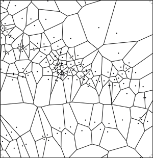
Figure 2 shows a 2-D particle distribution identical to figure 1(c) and a magnified view with a corresponding Voronoi diagram. We can observe that Voronoi cells of particles in clusters are relatively small, while those corresponding to particles outside clusters are large.

Figure 2. Voronoi tessellation generated by particles for  $St = 1$. Two-dimensional particle distribution in a slice of thickness
  $4\eta$ (a), corresponding to a zoom of figure 1(c). A magnified view with Voronoi tessellation (b).
4. Numerical results
In the following we present numerical results for inertial particles in isotropic turbulence considering seven different Stokes numbers. Fluid particles are likewise analysed, which allow us to understand the statistical properties and to assess the numerical precision of the divergence approximation in (3.3).
We compute the Voronoi volume for different Stokes numbers and we compare statistical properties with those obtained for random particles. Figure 3(a) shows the PDF of the Voronoi volumes  $V_p$, which is normalised by the mean volume
  $\overline {V_p}=(2{\rm \pi} )^{3}/N$. For randomly distributed particles, the PDF of the Voronoi volume becomes a gamma distribution (Ferenc & Néda Reference Ferenc and Néda2007). For the 3-D case, the PDF of the Voronoi volume is given by
  $\varGamma (5,1/5)$, where
  $\varGamma (k,\theta )$ corresponds to the PDF
  $f_{Vp}(x)=\varGamma (k)^{-1}\theta ^{-k}x^{k-1}\exp (-x/\theta )$ and where
  $k$ and
  $\theta$ are shape and scale parameters, respectively. In figure 3(a) we have confirmed that the PDF for randomly distributed particles in our results agrees well with the gamma distribution of
  $\varGamma (5,1/5)$. We can see that, as the Stokes number increases and is getting closer to
  $1$, the number of small Voronoi cells for
  $V_p/\overline {V_p} \lesssim 0.5$ increases, and then decreases after exceeding
  $St = 1$. The number of the large Voronoi cells increases as the Stokes number increases and it stabilises. The PDF of the Voronoi volume is often used to determine ‘cluster cells’ and ‘void cells’. Monchaux et al. (Reference Monchaux, Bourgoin and Cartellier2010) adopted the intersection of the PDF of the Voronoi volume and the gamma distribution as thresholds. A Voronoi cell smaller than the smaller threshold (the left intersection) is defined as a cluster cell, and, similarly, a Voronoi cell larger than the larger threshold (the right intersection) is defined as a void cell. In our results, the threshold to determine cluster cells is
  $V_p/\overline {V_p} \sim 0.5$.

Figure 3. Probability distribution functions of (a) Voronoi volume normalised by the mean and (b) divergence for particle velocity for different Stokes numbers and for randomly distributed particles ( $St=0$). The inset of (a) compares the PDF for randomly distributed particles with the gamma distribution. The inset of (b) shows the probability distribution functions for positive divergence values in log-log representation.
The divergence of the particle velocity is then computed using (3.3). Figure 3(b) shows the PDF of the divergence of the particle velocity. The probability distribution functions are almost symmetric, centred around 0 with stretched exponential tails.
Table 1 shows the variance and flatness of the divergence  ${\mathcal {D}}_p$ as a function of the Stokes number. The variance of the divergence increases as the Stokes number increases. For small Stokes numbers (
 $St \le 0.2$), the variance is strongly reduced. The flatness of the divergence first increases with
  $St$, reaches its maximum value around
  $St=0.5$ and then decreases again. This observation suggests that the tails decay faster for larger
  $St$. To understand which part of the divergence of the particle velocity is due to a geometrical error, we added the PDF of the divergence of the fluid velocity (
 $St=0$). Note that for fluid particles in the continuous setting, the divergence of the fluid velocity vanishes exactly, whereas in the discrete setting
  ${\mathcal {D}}_p$ differs from zero, because the deformation of a Voronoi cell is not exactly the same as the deformation of a fluid volume in the continuous setting. For the divergence of the fluid velocity, we find indeed values ranging between
  $-150$ and
  $+150$. Hence, we can deduce that for Stokes numbers less than
  $0.2$, the divergence is mostly due to a geometrical effect, but for larger Stokes numbers, physical effects predominate. The numerical precision of the divergence computation has been assessed in appendix A. In appendix B the geometrical effect on the divergence is further discussed for the case of randomly distributed particles.
Table 1. Variance and flatness of divergence  ${\mathcal {D}}_p$ as a function of the Stokes number.

To get further insight into the cluster formation, we plot the joint PDF of the divergence  ${\mathcal {D}}_p$ and the Voronoi volume
  $V_p$ normalised by its mean. Figure 4 shows the joint PDF for the cases of
  $St=1$ and 5 where the variance of
  ${\mathcal {D}}_p$ for inertial particle velocity is larger than that for fluid velocity. For these Stokes numbers, high probability is found along the line of
  ${\mathcal {D}}_p=0$. This indicates that a large number of the particles has quite small divergence, e.g. the divergence of 48.5 % of particles for
  $St=1$ is smaller than the standard deviation for
  $St=0$. This means that a group of local particles moves together like an incompressible flow. We can find large variance of the divergence that corresponds to the variance shown in figure 3(b). Such high probability of large positive/negative divergence is observed for cluster cells (
 $V_p/\overline {V_p} \lesssim 0.5$). A possible reason is that the probability of finding particles in cluster regions is higher than in void regions, as shown in figure 3(a). Another possible explanation is that the ‘caustics’ (Wilkinson & Mehlig Reference Wilkinson and Mehlig2005) of the particle density, where the particle velocity at a single position is multi-valued, result in a large velocity difference of two particles with a small separation distance and cause the extreme divergence values observed in the joint probability distribution functions.

Figure 4. Joint PDF of the volume of Voronoi cells in log scale and divergence in linear scale for (a)  $St=1$ and (b)
  $St =5$.
One would expect that particles in clusters are more likely to experience negative divergence. However, to maintain the statistically stationary state of the PDF of Voronoi volumes, positive divergence values must be comparable to the negative divergence values in clusters. If cluster volumes showed only negative divergence (cluster formation) and void volumes showed only positive divergence (void formation), particles would concentrate at infinitesimal volumes at the end, i.e. cluster destruction and void destruction are necessary for a statistically dynamic equilibrium.
In figure 4 it is also observed that large positive divergence values are mostly found at smaller volumes compared to large negative divergence values. This trend becomes more pronounced as the Stokes number increases and suggests asymmetry of the probability of positive and negative  $\mathcal {D}_p$. The larger probability of positive values of
  $\mathcal {D}_p$ for small volumes (particles in clusters) is attributed to the crossing motion of particles in clusters. When two particles are approaching each other the divergence is negative, but if two particles have large relative approaching velocities the particles start leaving from each other within the finite time
  ${\rm \Delta} t$ and the divergence changes to positive. This would happen prominently in caustic regions. As the Stokes number increases, the deviation of particle motion from fluid flow becomes larger and the relative particle velocity increases. Thus, the influence of the crossing motion of particles is more pronounced. These results further suggest that cluster formation is driven by the underlying flow field, but the cluster formation coincides with cluster destruction in a fine cluster with the dissipation scale. Thus, the divergence and convergence of particles in clusters are not determined only by the underlying flow field. To confirm that, we coloured in figure 1 each particle by its divergence value
  $\mathcal {D}_p$. It is observed that particles with large positive and negative values are concentrated in fine clusters, and, thus, the cluster formation coincides with cluster destruction, as expected. Particles with large positive/negative divergence are found not in all clusters, but some portion of clusters have only moderate divergence. That is, there are two types of clusters, those associated with strong cluster formation and cluster destruction and those which are formed and destroyed by modest change. Figure 1 further illustrates that the clusters with strong formation and destruction are intermittently distributed for all Stokes numbers, even for the case of
  $St \le 0.2$, and the portion of such clusters seems to increase as the Stokes number increases.
We also compute the mean of the divergence as a function of the volume which corresponds to the conditional average of the divergence, defined as
 \begin{equation} \langle {\mathcal{D}}_p \rangle_{Vp} = \frac{1}{P(V_p/\overline{V_p})} \int_{-\infty}^{+\infty} {\mathcal{D}}_p P({\mathcal{D}}_p,V_p/\overline{V_p}) \, \textrm{d}{\mathcal{D}}_p , \end{equation}
and shown in figure 5(a). Negative values correspond to convergence of the particles and positive values to divergence. We can see that the mean of the divergence  $\langle {\mathcal {D}}_p \rangle _{Vp}$ is negative for large volumes and turns to positive as the volume becomes smaller. This indicates that the cluster formation is active for large volumes, while cluster destruction/void formation is active for small volumes. For the considered Stokes numbers, the zero-crossing points are
  $V_p/\overline {V_p} \approx 0.1\text {--}0.2$. This can be expressed in terms of the dissipation scale
  $\eta$ of the flow which is
  $\eta = 7.9 \times 10^{-3}$. Using the relation
  $\overline {V_p}/\eta ^{3} = (2{\rm \pi} )^{3}/(N_p \eta ^{3}) \approx 33.54$, we can conclude that the scales of the zero-crossing point are ranging in
  $V_p^{1/3}/\eta \approx 1.49\text {--}1.88$. Moreover, we observe that when the Stokes number increases, the divergence takes larger values for both negative and positive sides. This means that the cluster formation becomes intensified as the Stokes number increases, and the cluster destruction for small volumes is also amplified. That is, when the Stokes number increases, for
  $V_p/\overline {V_p} \gtrsim 0.2$, cluster formation is intensified, whereas for
  $V_p/\overline {V_p} \lesssim 0.2$, cluster destruction is intensified. Strong cluster destruction suggests that clusters are destroyed before they become finer clusters. This is consistent with the fact that fine clusters are less observed as the Stokes number becomes larger than one.

Figure 5. Mean divergence  $\langle {\mathcal {D}}_p \rangle _{Vp}$ (a) and skewness (b) as a function of the Voronoi volume for different Stokes numbers. A moving average filter has been applied for the skewness. The inset shows a zoom to illustrate the presence of negative values.
The difference in magnitude between positive and negative values of the conditional divergence in figure 5(a) can be related to the second-order velocity structure function  $S_2(r) = \langle |u(x+r) - u(x)|^{2} \rangle$. For isotropic turbulence, we have
  $S_2(r) \propto C_2 r^{2/3}$ for
  $\eta \ll r \ll l _E$ (where
  $l_E$ is the energy scale) and
  $S_2(r) \propto r^{2}$ for
  $r \ll \eta$. The structure function of the inertial particle velocity is similar to the one of the fluid velocity for
  $\eta \ll r \ll l_E$, for
  $r \ll \eta$ it deviates from
  $r^{2}$-scaling and does not approach zero for finite Stokes numbers (Salazar & Collins Reference Salazar and Collins2012; Ireland, Bragg & Collins Reference Ireland, Bragg and Collins2016). This means that for
  $r \gg \eta$, the r.m.s. particle velocity difference is
  $\sqrt {\langle |\delta v|^{2} \rangle } \propto r^{1/3}$. Thus, the increase of the velocity difference with
  $r$ is statistically slower than the increase of the separation distance
  $r$, i.e.
  $\mathcal {D}_p \sim \sqrt {\langle |\delta v|^{2} \rangle }/r$ decreases with
  $r$. For
  $r \ll \eta$,
  $\mathcal {D}_p \sim \sqrt {\langle |\delta v|^{2} \rangle }/r$ increases with decreasing
  $r$ because the r.m.s. particle velocity difference at zero separation distance has a finite value for inertial particles. Thus, the absolute values of divergence decrease as the volume increases.
To quantify the asymmetry of the joint probability distribution functions in figure 4, we plot in figure 5(b) the skewness of the divergence as a function of the Voronoi volume. We observe a similar trend, positive values for small volumes and negative values for large volumes, for the shown Stokes numbers. The negative values of the skewness are more significant than those of  $\langle {\mathcal {D}}_p \rangle _{Vp}$, and, thus, we can confirm the asymmetry of the joint PDF at intermediate volumes in the range more clearly, e.g. for
  $St=1$ from
  $V_p/\overline {V_p} = 10^{-1}$ to almost
  $10^{1}$. For all Stokes numbers,
  $\langle {\mathcal {D}}_p \rangle _{Vp} \approx 0$ and the skewness is close to zero for
  $V_p/\overline {V_p} > 10^{2}$. This indicates that the joint PDF is symmetric, which suggests that void formation almost balances void destruction.
5. Conclusions
Voronoi tessellation of the particle positions was applied to different homogeneous isotropic turbulent flows at high Reynolds numbers computed by 3-D direct numerical simulation. Random particles and inertial particles with different Stokes numbers were considered. For analysing the clustering and void formation of the particles, we proposed to compute the volume change rate of the Voronoi cells and we showed that it yields a finite-time measure to quantify the divergence. We assessed the numerical precision of this measure by applying it to fluid particles, which are randomly distributed without self-organisation due to the volume preserving nature of the fluid velocity. From this we concluded that sufficiently large Stokes numbers ( $St>0.2$) are necessary to obtain physically relevant results.
Considering the joint PDF of the divergence and the Voronoi cell volume illustrates that the divergence is most pronounced in cluster regions of the particles and much reduced in void regions. We showed that for larger volumes, we have negative divergence values which represent cluster formation (i.e. particle convergence) and for small volumes, we have positive divergence values which represents cluster destruction/void formation (i.e. particle divergence). Our results suggest that the divergence and convergence of particles in clusters are not determined only by the underlying flow field, and the detailed features will be analysed in future work.
Finally, our results indicate that when the Stokes number increases the divergence becomes positive for larger volumes, which gives some evidence why for large Stokes numbers fine clusters are less observed for Stokes number larger than one.
The idealized situation in the present work considering point particles and one-way coupling at moderate Reynolds number can be extended in different directions. Studying the dynamics in the inertial range of particle-laden very large-Reynolds-number flows is an interesting perspective, the application to flows with finite size particles taking into account two-way (or four-way) coupling is likewise challenging. The proposed method for determining the divergence of the particle velocity can be also applied (within some limitation due to the discretization) to lower seeding density situations encountered in experiments. Hence, our approach is more general and can be applied to experimental and DNS data in more complex situations.
Acknowledgements
T.O. acknowledges financial support from I2M. K.M. thanks financial support from JSPS KAKENHI grant number JP17K14598 and I2M, Aix-Marseille University for kind hospitality. K.S. thankfully acknowledges financial support from the Agence Nationale de la Recherche (ANR grant number 15-CE40-0019), project AIFIT and thanks JAMSTEC for financial support and kind hospitality. Centre de Calcul Intensif d'Aix-Marseille is acknowledged for granting access to its high performance computing resources. The DNS data analysed in this project were obtained using the Earth Simulator supercomputer system of JAMSTEC. The authors thank K. Yoshimatsu and S. Apte for constructive comments and fruitful discussion.
Declaration of interests
The authors report no conflict of interest.
Appendix A. Numerical precision of the divergence computation
A.1. Reliability of the method
To assess the reliability of the discrete Voronoi-based divergence computation proposed in (3.3), we consider a stationary periodic velocity field  ${\boldsymbol u}$ in two space dimensions, which has no vanishing divergence. We inject
  $N_p = 10^{5}$ randomly distributed fluid particles into the
  $2 {\rm \pi}$-periodic square domain and advect them for one time step
  ${\rm \Delta} t =10^{-2}$ using the explicit Euler scheme. Then we apply Voronoi tessellation and compute the volume change of the Voronoi volumes according to (3.3).
Figure 6(a) superimposes the velocity field and its divergence, and figure 6(b) gives the absolute value of the divergence error in log scale. We observe that the error is most important in strain dominated regions. Hence, we compute the strain rate of the flow,  $s_{ij}s_{ij} = 2\cos ^{2}{x}\sin ^{2}{y}$, where
  $s_{ij}=(\partial _j u_i +\partial _i u_j)/2-\delta _{ij}\partial _k u_k/2$. As the correlation between the magnitude of the divergence error and the strain rate is nonlinear, we decided to use the Spearman correlation coefficient instead of the Pearson one. We find reasonably well agreement with strong correlation-ship reflected in the value
  $r_s = 0.683$.

Figure 6. Velocity field  ${\boldsymbol u}(x, y) = (\cos (x)\cos (y), -\sin (x)\sin (y))$ superimposed with its divergence
  $\boldsymbol {\nabla } \boldsymbol {\cdot } {\boldsymbol u}(x, y) = -2\sin (x)\cos (y)$ (a). Difference between the exact divergence and the discrete Voronoi divergence in log scale (b). Joint PDF of the exact divergence and the discrete Voronoi divergence, together with the one-dimensional (1-D) probability distribution functions of the exact divergence and the Voronoi divergence (c). Pearson correlation coefficient between exact and Voronoi divergence as a function of the number of particles
  $N$ with limit value
  $r = 0.936$, represented by box plots (d). The horizontal line is the median, the upper and lower box are respectively the first and the third quartile, and the top and bottom lines are the largest and the lowest data points, respectively, excluding any outliers.
The joint PDF of the exact divergence and the discrete Voronoi divergence in figure 6(c) illustrates nicely the strong correlation between the two quantities, as expected. To quantify this correlation, we plot in figure 6(d) the Pearson correlation coefficient for an increasing number of particles, i.e. from  $N = 10^{3}$ to
  $10^{4}$ with
  $15$ values distributed equidistantly in log scale. Shown are box plots indicating the median, and boxes with the first and third quartile to quantify the variability together with min/max values. After a monotonous increase, we observe for
  $N \ge 4\times 10^{3}$ a saturation at the value of
  $r = 0.936$, which confirms the strong correlation and also shows that the error does not tend to zero when increasing the number of particles further. However, for an increasing number of points, the variability is strongly reduced.
To summarise, the above discrete divergence results for particles in a given divergent 2-D flow are in good agreement with the exact values of the divergence of the carrying flow field. This shows that the proposed finite-time Voronoi tessellation-based method is well suited and reliable for computing the divergence of the particle velocity.
A.2. Robustness of the method
To verify the robustness of the discrete Voronoi-based divergence computations, we consider again the previously presented 3-D DNS data for  $St=0$ and
  $1$. We check the influence of the time step
  ${\rm \Delta} t$ and of the number of particles
  $N$ on the statistics of the computed discrete divergence of the carrying flow field. Note that in the DNS we have
  $N = 1.5 \times 10^{7}$ and
  ${\rm \Delta} t =10^{-3}$.
Figure 7 shows the PDF of the divergence  $\mathcal {D}_p$ for different values of
  ${\rm \Delta} t$ and
  $N$. For
  $St=0$, the probability distribution functions remain almost unchanged and perfectly superimpose when dividing or multiplying the time step by a factor two, or dividing the number of particles by two, which proves the robustness of the statistics for fluid particles. For
  $St=1$, the situation changes with the exception of time step reduction, while keeping
  $N$ fixed. Replacing
  ${\rm \Delta} t$ by
  ${\rm \Delta} t/2$ yields an almost identical distribution. This shows that the time step has been chosen sufficiently small. Increasing
  ${\rm \Delta} t$ to
  $2 {\rm \Delta} t$, while keeping
  $N$ fixed, some dependence is found for
  $|\mathcal {D}_p|>500$ and the tails suddenly decay around
  $\mathcal {D}_p = \pm 1000$. This can be explained by the CFL condition for the volume change:
  $|D_t V_{p}| {\rm \Delta} t/V_{p} < O(1)$. The divergence is given by
  $\mathcal {D}_p = D_t V_{p}/V_{p}$. Thus,
  $\mathcal |D_p| < O(1/{\rm \Delta} t)$ would satisfy the CFL condition.

Figure 7. Probability distribution function of the divergence,  ${\mathcal {D}}_p$, for (a)
  $St = 0$ and (b)
  $St = 1$ for three time steps
  ${\rm \Delta} t = 10^{-3}$,
  $2 {\rm \Delta} t$ and
  ${\rm \Delta} t / 2$, and two numbers of particles
  $N$ and
  $N/2$. Moving average smoothing was applied.
The  $N$ dependence of the divergence is due to the
  $N$ dependence of the mean separation length
  $l$. The sampling density becomes coarser as
  $N$ decreases, and then the Voronoi tessellation results loose the information at fine scales. This is reflected in lighter tails in the PDF for
  $N/2$ compared to the one obtained with
  $N$ particles. However, the extreme values are not significantly modified. Thus, the
  $N$ dependence can be considered as the difference in the sampling density. The divergence at caustic regions would be also sensitive to the sampling density.
A.3. Geometrical effect
To quantify the influence of the Voronoi tesselation, we computed the variance of the discrete divergence for  $St=0$, 0.1, 0.5, 1 and 5 for a varying number of particles from
  $N/8192$ to
  $N$, the results are shown in figure 8.

Figure 8. Variance of the computed discrete divergence  ${ \mathcal {D}}_p$ for
  $St = 0$, 0.1, 0.5, 1 and
  $5'$ as a function of the number of particles
  $N_p = N$,
  $N/2$,
  $N/4$,
  $N/8$,
  $N/16$,
  $N/32$,
  $N/128$,
  $N/1024$,
  $N/2048$,
  $N/4096$ and
  $N/8192$, where
  $N = 1.5 \times 10^{7}$.
For fluid particles,  $St=0$, the variance of the divergence
  $\mathbb {V} ({\mathcal {D}}_p)$ should be equal to
  $0$ for any number of particles. Figure 8 illustrates that this is not the case. The variance for
  $St=0$ even grows with
  $N$ and then saturates for
  $N>10^{6}$. This error is due to geometrical effects: the error appears because the deformation of Voronoi cells is not the same as the one of the fluid. We remark that for particles on a Cartesian grid this geometrical effect is absent. Note that the geometrical effect does not decrease even when we further increase the number of particles for
  $St=0$ because the geometrical effect of deformation remains also for smaller Voronoi cells. Comparing the cases
  $St=0$ and
  $St=0.1$, we find almost identical values for the variance for
  $N<10^{5}$. However, for
  $N>10^{6}$, the variance values for
  $St=0.1$ are larger than those for
  $St = 0$. This difference is brought about by a physical effect.
To explain the  $N$ dependence of the variance, we introduce the particle separation scale
  $l=\overline {V_p}^{1/3} = 2{\rm \pi} N^{-1/3}$ and the corresponding wavenumber
  $k_N \equiv 2{\rm \pi} /l = N^{1/3}$. The energy spectrum of turbulence shows strong decay for
  $k \eta \gtrsim 1$. In order to resolve fluid flows in the dissipation scale, the particle separation
  $l$ should satisfy
  $k_N\eta > 1$, which is given by
  $N > 2.03 \times 10^{6}$. This explains why the variance for
  $St=0$ is constant for
  $N>10^{6}$ in figure 8. For the cases of
  $0<St<1$, the clustering particle dynamics occur mainly at the scale smaller than the dissipation scale. Hence,
  $k_N\eta > 1$ gives the minimum number of particles to observe the difference from the case of
  $St=0$, i.e. the number of particles in the volume of
  $\eta ^{3}$ should satisfy
  $n\eta ^{3} > (2{\rm \pi} )^{-3}$. For
  $St\ge 1$, the clustering is more significant and there is no minimum scale (as illustrated in the number density spectrum in Matsuda et al. Reference Matsuda, Onishi, Hirahara, Kurose, Takahashi and Komori2014). Thus, it is challenging to determine the minimum number of particles for an arbitrary Stokes number.
The difference of the variance implies that the divergence for  $St\le 0.1$ is not fully dominated by the geometrical effect. Table 2 shows the percentage of particles for which the magnitude of the divergence is below the standard deviation (with value
  ${std}= 4.571$) of the computed discrete divergence of the fluid particles (
 $St=0$). For
  $St \leq 1$, a large number of particles has a divergence smaller than the standard deviation of the computed discrete divergence of the fluid particles. However, a certain amount of particles shows significantly large divergence values.
Table 2. Percentage of particles with the magnitude of the divergence below the standard deviation of the discrete divergence of fluid particles ( ${std}= 4.571$).
A.4. Fluid particles: influence of sampling
For fluid particles ( $St=0$) in the continuous setting, the divergence of the fluid velocity vanishes exactly, while in the discrete setting
  ${\mathcal {D}}_p$ differs from zero. The reason is that the deformation of a Voronoi cell is not exactly the same as the deformation of a fluid volume in the continuous setting. The fluid particles of
  $St=0$ are sampled homogeneously in space, while the inertial particles are distributed inhomogeneously. To check the influence of the sampling of the fluid velocity, we use the Voronoi tessellation for eight Stokes numbers
  $St=0$, 0.05, 0.1, 0.2, 0.5, 1, 2 and 5. Then we compute the divergence of the fluid velocity using the volume change of the corresponding Voronoi tessellation.The resulting probability distribution functions of the divergence of the fluid velocity are shown in figure 9. The divergence of fluid velocity for inertial particle positions has slightly heavier tails than that for homogeneous sampling. However, the divergence of the fluid velocity take values ranging between
  $-150$ and
  $+150$. This confirms that for Stokes numbers less than
  $0.2$, the divergence is mostly due to the geometrical effect, and for larger Stokes numbers, the divergence of the particle velocity is a physical effect with values significantly larger.

Figure 9. Probability distribution function of divergence of the fluid velocity using Voronoi tessellation of the particle positions for  $St=0$, 0.05, 0.1, 0.2, 1, 2 and 5.
Appendix B. Randomly distributed particles
To quantify the geometrical error of the divergence estimation, we consider first a simple toy model in one dimension. We consider randomly distributed particles and move them randomly to the left and to the right on the line. We assume that the particle velocity satisfies a normal distribution with zero mean and variance  $\sigma ^{2}$, i.e.
  $v_p \sim \mathcal {N}(0,\sigma ^{2})$. The volume change
  $D_t V_p$ is given by the relative velocity of neighbour particles:
  $D_t V_p = (v_{p,{right}} -v_{p,{left}})/2$, and, thus, the PDF of the normalised volume change
  $(D_t V_p)^{*} \equiv D_t V_p/v_0$ exhibits
  $\mathcal {N}(0,\sigma '^{2})$, where
  $\sigma '={\sigma }/{\sqrt {2} v_0}$ and
  $v_0$ is the representative particle velocity. The Voronoi volume satisfies a gamma distribution
  $\varGamma (k,\theta )$ with shape parameter
  $k=2$ and rate
  $\theta =1/2$, i.e.
  $V_p^{*} \equiv V_p/\overline {V_p} \sim \varGamma (2,1/2)$. The PDF of the normalised divergence
  $\mathcal {D}_p^{*} \equiv \mathcal {D}_p/(\overline {V_p}^{-1} v_0)$ is then given by the product distribution of two independent random variables
  $X=(D_t V_p)^{*} \sim \mathcal {N}(0,\sigma '^{2})$ and
  $Y={V_p^{*}}^{-1} \sim \varGamma ^{-1}(2,2)$, where
  $\varGamma ^{-1}(k,1/\theta )$ is the inverse gamma distribution defined as
  $f_Y(y) = ({\theta ^{-k}}/{\varGamma (k)})({1}/{y^{k+1}})\exp (-1/(\theta y))$. Note that we consider the absolute value of the divergence because the PDF of the divergence is symmetric in this case. Using the scaled complementary error function
  $\textrm{erfcx}(x) \equiv \textrm {e}^{x^{2}}\{1 - \textrm{erf}(x)\}$, where
  ${\rm erf}(x)$ is the error function, we finally obtain the expression for the PDF of
  $Z=|\mathcal {D}_p^{*}|$,
 \begin{equation} f_{|\mathcal{D}p^{*}|}(z) = \frac{K_1}{2z^{5}}\left( \sqrt{2{\rm \pi}}\sigma'^{3}(4\sigma'^{2}+z^{2}) \textrm{erfcx}\left( \frac{\sqrt{2}\sigma'}{z}\right) - 4\sigma'^{4}z \right), \end{equation}
where  $K_1$ is a normalisation constant.
Figure 10(a) shows the PDF corresponding to the ratio of a normal and a gamma distribution, given by (B 1), in red and the PDF obtained using Monte–Carlo simulations with  $10^{7}$ particles. We find perfect agreement between the theory and the numerical simulation.

Figure 10. Probability distribution function of the divergence of the particle velocity using Voronoi analysis in (a) one dimension and in (b) three dimensions. Shown are the theoretical PDF  $f_{|\mathcal {D}_p|}$, the Monte–Carlo (M-C) simulation results for Voronoi cells advected by a velocity satisfying a normal law and in the 3-D case additionally the DNS results for fluid particles,
  $St=0$. The vertical line corresponds to 99 % probability. The insets show the corresponding probability distribution functions of the normalised volume changes: Monte–Carlo simulations (green) and
  $St=0$ (dashed line) in three dimensions, together with fits for the normal (red) (with parameter
  $\sigma = 3.06$) and logistic distribution (blue) (with parameter
  $s = 1.84$), respectively.
The above model for the divergence of random particles can be extended to three dimensions. In three dimensions the divergence is normalised as  $\mathcal {D}_p^{*} \equiv \mathcal {D}_p/(l^{-1} v_0)$, where
  $l$ is the mean particle distance
  $l \equiv \overline {V_p}^{1/3}$. Similarly to the 1-D case, we consider the product distribution of two independent random variables
  $X=|(D_t V_p)^{*}|$ and
  $Y={V_p^{*}}^{-1}$, assuming
  $(D_t V_p)^{*} \equiv D_t V_p/(l^{2} v_0) \sim \mathcal {N}(0, \sigma '^{2})$ and
  ${V_p^{*}}^{-1} \sim \varGamma ^{-1}(5, 5)$. The resulting PDF of
  $Z=|\mathcal {D}_p^{*}|$ becomes
 \begin{align} f_{|\mathcal{D}_p^{*}|}(z) &= K_3 \left(\frac{\sigma'}{z}\right)^{6} \left[ 8 +9\left(\frac{5\sigma'}{z}\right)^{2} + \left(\frac{5\sigma'}{z}\right)^{4} \right. \nonumber\\ &\quad \left. - \left\{ 15 +10\left(\frac{5\sigma'}{z}\right)^{2} +\left(\frac{5\sigma'}{z}\right)^{4}\right\} \sqrt{\rm \pi}\left(\frac{5\sigma'}{\sqrt{2}z}\right)\operatorname{erfcx}\left( \frac{5\sigma'}{\sqrt{2}z} \right) \right], \end{align}
where  $K_3$ is the normalisation constant for the 3-D case. Note that evaluating this expression numerically is ill conditioned and some identities and approximations need to be used for stabilisation.
Figure 10(b) shows that the PDF obtained with the Monte–Carlo simulation perfectly superimposes with the theoretical prediction (B 2) for values smaller than  $\approx 10^{1}$. For larger values, the two curves exhibit some deviation and the observed small deviation is certainly due to the approximation made in Ferenc & Néda (Reference Ferenc and Néda2007) concerning the choice in the parameters of the gamma distribution. The insets in figure 10 show the probability distribution functions of the time change of the Voronoi volume for the 1-D and 3-D cases, respectively. In one dimension we observe a perfect superposition of the Monte–Carlo results with the normal distribution, while in three dimensions this is not the case. A better fit is observed for the logistic distribution. A possible explanation of the heavy tails in the PDF for the 3-D case is that the variance of the volume change becomes larger as the Voronoi volume increases. This happens because the larger Voronoi volume tends to have a larger surface area. Large variance of the volume change at large volume then causes heavier tails in the PDF of the volume change than the normal distribution, because the gamma function has an exponential tail.


