
Introduction
Why do some countries have higher CO2 emissions than others that are at least as economically developed and are no more advantaged in terms of technological possibilities? In a Data Envelopment Analysis (DEA) framework (e.g. Zofio and Prieto Reference Zofio and Prieto2001; Zhou et al. Reference Zhou, Wah Ang and Han2006, Reference Zhou, Wah Ang and Leng Poh2008a, Reference Zhou, Wah Ang and Leng Poh2008b, Reference Zhou, Leng Poh and Wah Ang2010), such states do not achieve the benchmark for carbon efficiency set by comparable states. They have failed to reach the carbon efficiency frontier: conditional on their level of development and the structural patterns of production and consumption that go with it, these countries have not reduced emissions as far as possible given the technological possibilities.Footnote 1
The aim of this article is twofold. First, we present a new outcome measure, Environmental Input Efficiency, which captures countries’ distance from the carbon emission efficiency frontier, benchmarking them against comparable states. Diffusing from the application of management science in the private sector to the portfolio of “new public management” techniques, the literature now increasingly and widely applies benchmarking (Francis and Holloway Reference Francis and Holloway2007; Triantafillou Reference Triantafillou2007). In the long term, structural factors may change and technological possibilities should open up; hence, our efficiency measure captures whether states have fully exploited possibilities for progress on climate change in the short to medium term. Second, a key question is, however, what public policies are effective in bringing about such progress. To address this, our research question concerns green taxation, which is among the most important environmental policy instruments. We test the hypothesis that the higher the revenue from green taxes, the greater a state’s input efficiency, as we expect that green taxation leads to improved performance relative to a state’s benchmark. Hence, this article makes two central contributions to the literature as we introduce an innovative measure for environmental quality and systematically study how this is influenced by one of the most important national policy tools in the environmental context. We hope that this research, thereby, sheds new light on the debate about how to capture environmental quality at the outcome level, and which factors affect this in certain ways.
Ever since Pigou (Reference Pigou1920) suggested that environmental externalities should be internalised by making polluters pay, economists have advocated market-based forms of regulation, including environmental taxation (OECD Reference Oates1999, 2008; Stavins Reference Stavins2003; Fujiwara et al. Reference Fujiwara, Núñez Ferrer and Egenhofer2006). The OECD (Reference Oates1999, 56), which has been at the forefront of promoting market-based regulation since the 1980s, defines environmental taxes as “any compulsory, unrequited payment to general government levied on tax bases deemed to be of particular environmental relevance. Taxes are unrequited in the sense that benefits provided by government to taxpayers are not normally in proportion to their payments”. They are held to be more efficient than forms of regulation that impose uniform technological or end-of-pipe emission standards on polluters. In principle, the same effects and efficiency gains can be achieved using various market-based policy instruments. Nonetheless, in practice, green taxation has advantages and disadvantages relative to “cap and trade” policies under which a market is created in emission permits (Stavins Reference Stavins2003). Notably, green taxes are easier to apply to citizens, much of the transport sector and to small-scale industrial emitters because only large firms are likely to have the capacity to operate effectively in carbon markets. They also raise revenue, unlike many tradeable permit schemes.
The next section describes our new performance measure, Environmental Input Efficiency, following which we present the theory. The “double-dividend” debate in economics, which we rely on for developing our argument, gives some grounds for suggesting that is it is possible to reduce carbon emissions while simultaneously making the economy more efficient by recycling the revenue from green taxes to cut taxes that distort the economy (see Anger et al. Reference Anger, Böhringer and Löschel2010 for a recent meta-analysis; see also Ekins and Speck Reference Ekins and Speck1999; Jordan et al. Reference Jordan, Wurzel and Brückner2003; OECD 2008). Following a discussion of the research design, we present the results, suggesting that green taxation is, indeed, associated with higher levels of Environmental Input Efficiency. Several robustness checks presented in the supplementary files increase our confidence regarding this.
Environmental Input Efficiency
Previous work in political science largely focuses on variation in countries’ absolute levels of environmental performance, and not performance benchmarked relative to comparable states (e.g. Li and Reuveny Reference Li and Reuveny2006; Ward Reference Ward2006; Bättig and Bernauer Reference Bättig and Bernauer2009; Bernauer and Koubi Reference Bernauer and Koubi2009; Fiorino Reference Fiorino2011; López et al. Reference López and Palacios2011; Spilker Reference Spilker2012a, Reference Spilker2012b; Bernauer and Böhmelt Reference Bernauer and Böhmelt2013b; López and Palacios Reference López, Galinato and Islam2014; Cao and Ward Reference Cao and Ward2015). Typical absolute measures include levels of emissions per capita or per unit of gross domestic product (GDP) (e.g. Bernauer and Koubi Reference Bernauer and Koubi2009, Reference Bernauer and Koubi2012; Spilker Reference Spilker2012a, Reference Spilker2012b; Bernauer and Böhmelt Reference Bernauer and Böhmelt2013a, 2013Reference Bernauer and Böhmeltb), expert assessments of performance (e.g. Böhmelt and Pilster Reference Böhmelt and Pilster2010, Reference Böhmelt and Pilster2011; Böhmelt and Betzold Reference Böhmelt and Betzold2013; Grundig and Ward Reference Grundig and Ward2015), aggregate indices such as the Environmental Performance Index (e.g. Hsu et al. Reference Hsu, Ainsley and Emerson2016), or a sustainability measure such as ecological footprint (e.g. Ward Reference Ward2006, Reference Ward2008). Clearly, no single measure is ideal for all purposes. For instance, per-capita carbon emissions may help in developing ideas about a fair distribution of access to the global commons in the long term; and in the long term, the aim must be to reduce all countries’ absolute level of emissions, and not just to achieve a benchmark level of efficiency. Nevertheless, to judge whether a state is currently taking advantage of technological possibilities, given the structural constraints it faces, its performance needs to be compared with that of a reasonable benchmark to avoid the “comparing-apples-and-oranges” problem that sometimes besets benchmarking (Maleyeff Reference Maleyeff2003). A poor country with much lower absolute emissions may not be a relevant benchmark for a rich country. Indeed, the rich country may have made greater gains relative to what is possible in the short to medium term than a poor state with much lower absolute emissions. A key advantage of benchmarking over absolute measures is that it prompts us to ask questions about whether a country could realistically do better in short to medium term by adopting a different policy mix.
Following Färe et al. (Reference Färe, Grosskopf and Hernández-Sancho2004), DEA has gained substantial popularity in research on environmental quality (Zofio and Prieto Reference Zofio and Prieto2001; Zhou et al. Reference Zhou, Wah Ang and Han2006, Reference Zhou, Wah Ang and Leng Poh2008a, Reference Zhou, Wah Ang and Leng Poh2008b, Reference Zhou, Leng Poh and Wah Ang2010). However, thus far, little use has been made of DEA to benchmark national environmental performance, to which we extend its use. DEA compares each unit to a benchmark among the set of entities that are held to be reasonable comparators (Zhou et al. Reference Zhou, Wah Ang and Han2006, 115; Zhou et al. Reference Zhou, Wah Ang and Leng Poh2008a, 2), combining information into a single indicator (Zhou et al. Reference Zhou, Wah Ang and Leng Poh2007, Reference Zhou, Leng Poh and Wah Ang2010). Specifically, our measure combines data on carbon emissions with data on structural constraints on decreasing emissions and on the availability of technology. The second and third factors enter the definition of the group of comparators, as we now explain.
Structural constraints have come under intense scrutiny in the literature on the Environmental Kuznets Curve (EKC) from which we derive ideas about what form they are likely to take. In turn, these ideas condition the way we will construct benchmarks. Structural factors are those that are difficult for a government to change in the short to medium term, and thus has to work within the constraints they impose. The EKC literature suggests that these constraints are associated with a country’s level of development and with technological possibilities. It is frequently argued that countries’ emissions of pollution first increase with development (GDP per capita) and then decline once a tipping point has been reached (e.g. Selden and Song Reference Selden and Song1994; Grossman and Krueger Reference Grossman and Krueger1995; Dasgupta et al. Reference Dasgupta, Laplante, Wang and Wheeler2002). The existence of such an EKC for carbon dioxide emissions is controversial, however. Some suggest that carbon emitted in producing exports should not count but carbon emitted in producing imports should (Aklin Reference Aklin2016), whereas others cast doubt on the econometric methods used to estimate relationships (Itkonen Reference Itkonen2012). Authors’ conclusions may depend on the sample of countries and the time period, as well as other factors it is deemed necessary to control for (for recent reviews, Harbaugh et al. Reference Harbaugh, Levinson and Wilson2002; Bernauer and Böhmelt Reference Bernauer and Böhmelt2013a; Kaika and Zervas Reference Kaika and Zervas2013a, 1395f; López-Menéndez et al. Reference López-Menéndez, Pérez and Moreno2014). In our sample, the estimated relationship between GDP per capita and per-capita CO2 emissions is monotonically increasing within the sample range of GDP per capita.Footnote 2 The structural relationship is that development increases per-capita emissions, but there is considerable variation around this pattern.
In the EKC literature the tendency for emissions to increase due to higher consumption consequent on greater income is termed the scale effect. The scale effect may be offset by compositional and technological effects (Kaika and Zervas Reference Kaika and Zervas2013a; López-Menéndez et al. Reference López-Menéndez, Pérez and Moreno2014). Compositional effects include shifts in the structure of production as manufacturing shrinks and the service sector grows, which may tend to reduce emissions (see Kaika and Zervas Reference Kaika and Zervas2013b, 1407f). Similarly, there are related shifts in the pattern of consumption with income, driven by similar income elasticity of demand for particular goods and services for countries with comparable levels of GDP per capita (Seale and Regmi Reference Seale and Regmi2006). Some shifts might increase emissions (e.g. increased demand for meat/dairy products with growing income) and some may reduce them (e.g. increased demand for “green products”). However, if there are negative impacts on emissions, they do not seem to be significant enough to counteract positive forces driving the structural patterns in our data.
If these patterns in production and consumption are regarded as structural, it follows that they are hard to change in the short to medium term. That said, government policy can affect carbon emissions within the constraints such structural patterns impose on making short-to-medium-term progress; and good policy should push as far as is feasible (Selden and Song Reference Selden and Song1994). For instance, green taxation of transport fuels might reorientate the structurally given high levels of demand for travel in richer countries away from using private cars towards public transport, resulting in lower emissions.
On the basis of evidence that technical change increases energy efficiency in the OECD (Adeyemi and Hunt Reference Adeyemi and Hunt2014; see also Jänicke Reference Jänicke1985, Reference Jänicke2008; Bernauer and Böhmelt Reference Bernauer and Böhmelt2013a; Dechezleprêtre and Glachant Reference Dechezleprêtre and Glachant2014), we assume that technology advances with time, allowing for the possibility of producing more with lower carbon emissions as years go by. For instance, according to the European Environment Agency, the efficiency of conventional electricity generation and heat production among European Union (EU)25 member states increased between 1994 and 2010 from around 42 to 57%.Footnote 3 We further assume that all countries have access to the current vintage of technology and to any technologies from previous years. One objection to this is that a country’s natural and geographical characteristics may make it unsuitable for using some technologies, for example, there may be no suitable sites for producing hydro-electric power. However, these are factors that do not change with time and can be dealt with by using fixed country effects in econometric models.Footnote 4
Moreover, lack of state capacity or corruption might make certain policies infeasible. Yet, a measure that attempts in part to benchmark political performance should not give an easier ride to a country because of such factors. Rather, they should be considered from a political-economy perspective as possible causal factors. In our sample, comprising OECD countries and a few other relatively rich countries for the period 1994–2011, we assume that governments have the capacity to adopt good practice in the absence of political barriers such as lobbying by heavy energy users or voter resistance.Footnote 5
Our measure, Environmental Input Efficiency, captures how much CO2 emissions per capita can be reduced given structural and technological constraints.Footnote 6 We assume that in our sample the structural constraints on reducing carbon emissions facing the government of a less-developed country are no greater than those facing a more developed country. We also assume that technological possibilities are at least as abundant at a later period of time than they were earlier. The cases we deal with are country-years. Denote country i in year t by i t . Then, the comparator group for i t consists of the set of country-years such that, for each member j t’ , t’⩽t and the GDP per capita of j t’ is at least as high as that of i t . In words, comparators in our understanding pertain to the set of country-years that (1) did not have access to more efficient energy technology and (2) were at least as highly developed, so that the structural problems governments faced in reducing emissions were at least as great.
DEA techniques differ in the use they make of information about the comparator group when calculating benchmarks and performance. We rely on “order-alpha” efficiency that generalises the free disposal-hull technique by allowing for measurement uncertainty about the output variable (Aragon et al. Reference Aragon, Daouia and Thomas-Agnan2005). Order-alpha computes nonparametric efficiency scores for decision-making units (Daraio and Simar Reference Daraio and Simar2007, 74; Zhou et al. Reference Zhou, Wah Ang and Leng Poh2008a, 2). It is a partial-frontier approach that does not envelop all data points by a nonconvex production-possibility frontier, but allows for some “superefficient” units to be located beyond the estimated frontier.Footnote 7 This has the advantage of reducing the effects of outliers in the data on efficiency scores (Tauchman Reference Tauchman2012).
The World Bank Development Indicators report CO2 emissions in kilotons from the burning of fossil fuels and the manufacture of cement, using information from the Carbon Dioxide Information Analysis Center. Emissions include carbon dioxide produced during the consumption of solid, liquid, gas fuels and gas flaring. We divide this item by a country’s midyear total population, which counts all residents regardless of legal status or citizenship (except for refugees not permanently settled) in order to obtain an estimate of CO2 emissions per capita. Second, we divide real GDP, that is, the sum of gross value added by all resident producers in the economy plus any product taxes and minus subsidies not included in the value of the products (in constant 2005 USD), by the same population item from the World Bank to obtain a measure of per-capita GDP.
Under the order-alpha approach, a given country-year is efficient (if not superefficient) if no more than 5% of other countries in the comparator group have (or had) lower carbon emissions, that is, the comparator at the 95th percentile for low CO2 emissions per capita is the benchmark for calculating efficiency in the year concerned. Environmental Input Efficiency is the ratio of CO2 emissions per capita of the benchmark to those of the country-year under study. These scores capture a state’s distance from the carbon efficiency frontier (see also Zofio and Prieto Reference Zofio and Prieto2001). Inefficient countries receive scores below 1, because their benchmark have lower emissions; efficient ones have scores of exactly 1; and superefficient states located beyond the estimated carbon efficiency frontier score above 1.
Figure 1 gives a visual impression of how order-alpha efficiency works. The data points are values of CO2 emissions per capita and GDP per capita of our sample in the year 2000. In general, inefficient countries are to the upper-left of efficient and superefficient countries, that is, they have a lower-income level but higher CO2 emissions. For example, consider the position of the United States (US) relative to Norway.Footnote 8 Note that relatively high CO2 emissions do not necessarily preclude a country from being efficient or superefficient. Norway falls into this category as it has a high-income level, but its comparator cases tend to have even higher CO2 emissions per capita. Hence, Figure 1 stresses again that we carry out benchmarking and not an absolute efficiency comparison. This is further emphasised by the correlation between CO2 emissions per capita and Environmental Input Efficiency, which is 0.73 (N=46) in 2000.Footnote 9 Although the two measures of performance correlate strongly, they do not capture the same underlying idea.
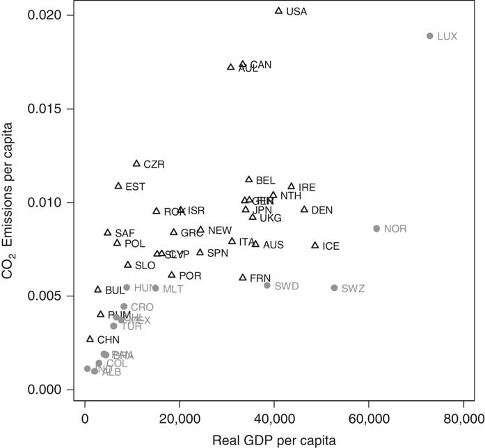
Figure 1 Environmental Input Efficiency (in the year 2000) Note: States with positions in grey (circles) have efficiency scores of 1 or more. States in black (triangles) are inefficient relative to their benchmark country and have scores below 1. The figure uses International Organisation for Standardisation abbreviations of country names. GDP=gross domestic product.
Absolute measures of environmental performance can fail to identify countries that could perform better. The key advantage of relative performance measures is that they help recognise such cases, which may alert us to possibilities for changing public policy. Partly because of its nuclear programme, France has lower absolute emissions of carbon than many other EU member states. For most of the period of our study (1994–2011), France is benchmarked against Switzerland (see the Online Appendix). Its average annual carbon emissions per capita were 0.0059 – only slightly higher than Switzerland’s at 0.0055 kt of per-capita CO2. However, Switzerland has on average a considerably higher real income ($53,962) than France ($33,672) in our sample period. If the structural relationship is that carbon consumption tends to increase as citizens become richer as the data in our sample suggests, these figures might lead us to question why France is not doing better, with an average input efficiency score of 0.95 against Switzerland’s 1.1. World Bank data show while Switzerland generated about 53.8% of its electricity from hydro-electric power about the mid-point of our period in 2002 (France: 10.9% in 2002), France generated much more of its electricity from nuclear power in this year – 78.9% versus Switzerland’s 41.6%. Thus, it is not obvious that either country’s public policies in relation to low-carbon electricity sources lie behind the difference in input efficiency scores. Providing definitive answers on this is beyond the scope of this research. However, our point is that the input efficiency comparison prompts us to ask relevant questions. For instance, we might examine whether it matters that a considerably higher percentage of passengers and freight are carried by rail in Switzerland than in France.Footnote 10
The order-alpha approach not only allows efficiency comparisons for countries with the same GDP per capita, but also comparisons across states at different levels of development (as indicated above; however, our sample is largely homogeneous in that respect, as we focus on a sample comprising OECD countries and a few other relatively rich countries for a relatively short time period). It does so by capturing how far away countries are from their own benchmark. Table 1 lists in alphabetical order the average input efficiency scores for all countries in our sample over the period 1994–2011. The US (0.29), Canada (0.34) and Australia (0.34) are characterised by environmental inefficiency (i.e. scores below 1), whereas some rapidly developing countries are highly efficient, for example, Albania, Brazil and Colombia. Note that the superefficient status of these states is neither surprising nor implausible: compared to other less-developed states in our sample, they have low per-capita carbon emissions.
Table 1 Environmental Input Efficiency scores of sample countries (average for 1994–2011)
Not all less-developed countries in our sample have low per-capita carbon emissions, suggesting they are not doing all that could reasonably be done. South Africa provides a challenging case for our methodology. Averaging over 1994–2011, it has the relatively low efficiency score of about 0.41. Its average real income over this period is $5,334, about 0.9 SD below the mean. Yet, its CO2 emissions per capita averaged 0.008, ranking it 33-highest out of 49 countries in our sample – higher than many more highly developed countries including the United Kingdom, France, Spain or Italy. South Africa has relatively high-carbon emissions for a number of reasons (Winkler and Marquand Reference Winkler and Marquand2009; Menyah and Wolde-Rufael Reference Menyah and Wolde-Rufael2010): its heavy reliance on coal as an energy source, which provides ca. 70% of its primary energy and results in about 87% of its carbon emissions; a development path reliant on an “energy-mineral complex” of highly energy-intensive production and processing of minerals; policies favouring this path of development such as low energy and electricity prices (ca. 40% of US prices in the four decades leading up to the turn of the century); and reliance on coal-to-oil synthetic fuel production for strategic reasons.
At first sight, it might seem that there is relatively little that the South African government could do in the short term. Because of the legacy of Apartheid, it is one of the most unequal societies in the world, with high levels of poverty and energy poverty that need to be addressed by increasing the energy consumption of the poor. Changing paths from the “energy-mineral complex” might take decades, could harm economic growth (Menyah and Wolde-Rufael Reference Menyah and Wolde-Rufael2010) and would be politically difficult. Thus, there is a sense in which the complex is a country-specific structural constraint. That said, the South African government aims to reduce its carbon emissions and to contribute towards international action on climate change. A range of policies that had yet to be developed to any great extent during the period of our study could have pushed it towards the efficiency frontier (Winkler and Marquand Reference Winkler and Marquand2009): energy conservation, renewables, importation of natural gas and hydro-electricity from other African countries, reducing implicit energy subsidies, and carbon taxes. Furthermore, Winkler and Marquand (Reference Winkler and Marquand2011) suggest that carbon taxes could help South Africa reduce its emissions without harming the economy if introduced in a way that was sensitive to the effect on poorer people and at an appropriate level arrived at through an adjustment process.
Some might accept that benchmarking helps indicate whether there are realistic chances of making short to medium-term progress while challenging our methodology. On the basis of the sort of evidence cited above, it seems unproblematic that technology advances towards greater energy efficiency. But it could be asked whether all countries have access to the current pool of technology given intellectual property rights over some of it are often vested in certain rich countries. Even for the poorer countries in our sample such as India or South Africa, we do not think our access assumption is too strained, although we agree that care would need to be exercised if very poor countries were also included.
Some may object to our assumption that richer countries face tighter structural constraints, because patterns of high-carbon consumption are hard to shift in the short to medium run. First, it is easy to think of cases where other structural constraints, peculiar to the country concerned, are important, for example, South Africa’s “energy-mineral complex”. Should we only compare South Africa with countries with a similar development pattern? We might well face problems finding comparable cases; and the same problem would recur in relation to, say, finding cases that are as advantaged by inland water transport as the Netherlands and Belgium. In our view, if general benchmarking across a large number of countries is the aim, it is better to avoid sui-generis structural factors when constructing the set of comparable countries that provide the counterfactual for potential progress.
Our sample includes countries that are in the World Bank’s high-income group and countries that are in lower-income groups (12.86% of all country-years in our sample belong to the low or lower-middle-income groups). It is logically possible that a country in the low-income category (e.g. India until 2006) could be benchmarked against a high-income country. This might seem inappropriate because there are qualitative differences across income groups – notably the overwhelming priority of development in a low and lower-medium-income countries. This has led India, for example, to emphasise development over dealing with climate change, although there are signs that its discourse is shifting (Thaker and Leiserowitz Reference Thaker and Leiserowitz2014) – not least in relation to its stance in relation to the Paris UNFCCC 2015 agreement. In practice, most lower-income group countries in most years of our sample are benchmarked against countries in the same income group. For instance, India is typically benchmarked against Brazil and occasionally against Colombia (see the Online Appendix). This is because the benchmark is at least as developed, but, for most countries that are inside the efficiency frontier, will have lower emissions per capita – a condition that will not generally be satisfied by a state in a higher-income group given the relationship between income and energy consumption. In the light of this, it is not surprising that our results on the effects of green taxation are robust to benchmarking countries only against ones in their income group, as we note in the Online Appendix.
Groups could be further narrowed by only including countries in the same income group over a narrower time frame, extending back a few years. A disadvantage of this approach compared to ours is that the number of comparator states would be likely to be small. Part of the point of benchmarking is that it prompts us to look for “good practice”. With small groups of comparators, we might not look very far. With a larger comparator set, it could be possible to question whether examples of “good practice” are relevant to an apparently inefficient state. On the other hand, we avoid the problem of making comparisons arbitrary by restricting comparator groups in ad hoc ways: comparing with all states that were at least as highly developed at an earlier period is, at least, based on the EKC and the structural form of the relationship between GDP per capita and per-capita emissions in our sample. While we prefer our approach, others may well want to define comparator groups differently, because they have different purposes in mind.
Besides level of development, there are other structural factors that are can be regarded as relevant. Geography, as it affects climate, is an obvious one. Some countries use more carbon because they have colder climates; but so could others with hotter (leading to demand for more refrigeration and air conditioning) or drier climates (so more energy in processing and transporting water is used). We acknowledge that there are other structural factors at work and that further research on benchmarking might find a way of incorporating them, at least when it comes to testing our hypothesis about the effects of green taxation, we can allow for the impact of truly exogenous factors like geography by including country fixed effects in models.
Theory: the “double-dividend” debate
At stake in the double-dividend literature is whether the improvements in environmental quality, which theory suggests can be brought about through introducing green taxation, must be bought at the price of reductions in other aspects of social welfare. If there was a consensus in the literature that green taxation did reduce welfare, posing our research question (i.e. whether green taxation helps states attain their efficiency benchmark) may not be appropriate: whatever the environmental benefits of green taxation, it might not be possible to maintain or even increase GDP per capita while using this policy instrument. If green taxation was introduced, the comparator group could increase in size as the policy changed with some poorer countries being additionally included. Thus, the benchmark could alter in a way that suggests the policy measure reduced efficiency, despite the fact that pollution fell. However, the double-dividend literature suggests that it is not clear from economic theory whether emission reductions come at a cost in terms of welfare loss. Moreover, existing empirical studies tend to suggest that welfare losses can be avoided if green taxes are applied in appropriate ways.
Following Goulder (Reference Goulder1994), it is conventional to distinguish between strong and weak versions of the double-dividend claim. The latter is the relatively uncontroversial one that returning environmental tax revenues as a lump sum to citizens leads to lower welfare than using them to cut distortionary taxes, such as employers’ social security payments, business taxes on profits or income taxes. The strong double-dividend claim, as introduced by economists like Tullock (Reference Tullock1967: 643) in the 1960s, states that as long as revenues are recycled to reduce distortionary taxes, environmental taxes not only reduce environmental damage but can also be introduced while maintaining or even increasing welfare.
Theoretical concerns about the double-dividend can stem from second-order effects of environmental taxation, considered in a general equilibrium framework (Bovenberg and de Mooij Reference Bovenberg and de Mooij1994a). Higher green taxes, ceteris paribus, reduce consumption of “environmentally dirty” products by increasing their price (see also Aghion et al. Reference Aghion, Dechezleprêtre, Hémous, Martin and Van Reenen2016). However, price increases reduce real wages. Suppose that green tax revenue is recycled to reduce income tax. This somewhat compensates for the welfare effects of higher prices on dirty goods, but as the demand for them is reduced, green taxes erode their own taxation base. Assuming the reform is revenue neutral, the government is required to maintain total tax take; hence, it cannot reduce labour taxes enough to compensate for the loss of welfare from higher prices. Moreover, as real wages decrease, as a net consequence of higher prices combined with slightly lower-income taxes, workers take more leisure; correspondingly, another economic “distortion” is induced. Bovenberg and de Mooij (Reference Bovenberg and de Mooij1994a) conclude that it is unlikely that environmental taxation can be introduced without reducing welfare and that, considering second-order effects, optimal green taxes may be too low to fully internalise the environmental externality. General equilibrium models typically find evidence for such tax-interaction effects so that green taxes raise distortions in the tax system, which in turn might reduce welfare (Oates 1995; Bovenberg and Goulder Reference Bovenberg and de Mooij2001). That said, when moving away from a static general equilibrium framework, theoretical conclusions may be more positive. For instance, Bovenberg and de Mooij (Reference Bovenberg and Goulder1994b) employ an endogenous growth model and show that environmental taxes can enhance growth when environmental damage causes considerable loss of production.
Although much of the theoretical literature remains skeptical about the strong double-dividend unless the existing tax system is highly distortionary (see Bosquet Reference Bosquet2000; Patuelli et al. Reference Patuelli, Nijkamp and Pels2005), simulations tend to draw different conclusions. Such models are typically parameterised using data from a particular economy and examine several packages combining an environmental tax at different levels with various ways of redistribution via revenue-neutral tax breaks. For instance, recent work on the US in a computable general equilibrium framework proposes that recycling revenue to employment taxes is less efficient in terms of increasing social welfare than using it to lower business taxation. This is because of the way that investment is encouraged and the price of capital services are reduced (Jorgenson et al. Reference Jorgenson, Goettle, Ho and Wilcoxen2015). Ekins et al. (Reference Ekins, Pollitt, Summerton and Chewpreecha2012) simulate the impact of meeting the EU’s 20-20-20 goalFootnote 11 through green taxation with revenue recycling via employers’ social security contributions and income tax. Higher prices consequent on taxes slow household income growth, but tax recycling pushes it upwards. While the predicted effects on GDP are small, they are positive.
Bosquet (Reference Bosquet2000) synthesises results from 56 simulations. Most of these studies point to the reduction of carbon emissions. If flexible labour markets are assumed so energy taxes do not increase wages and revenue is recycled to cuts in employment taxes, results may even suggest increases in employment. In addition, Patuelli et al. (Reference Patuelli, Nijkamp and Pels2005) present a statistical meta-analysis of 66 simulations. Most of this research is based on reducing employment taxes and finds that unemployment drops, but the magnitude of the effect is smaller than that on carbon emissions. Models show mixed results in relation to GDP, and the authors emphasise that this may be partially due to the type of modelling framework used. Where employment taxes are reduced, differences in findings could be due to different assumptions about the flexibility of labour markets, among other factors. However, the meta-analysis by Anger et al. (Reference Anger, Böhringer and Löschel2010) does not find this factor to significantly account for differences between simulations.
In the light of the indeterminate nature of this debate, it is remarkable that little use has been made of the available data to carry out cross-country comparative research on the determinants and impact of green taxation using statistical methods. On the basis of estimates of long- and short-run elasticity of demand, Sterner (Reference Sterner2007) concludes that higher fuel taxes in Europe have contributed to a considerably higher efficiency compared to the US. Leiter et al. (Reference Leiter, Parolini and Winner2011) study how green taxation affects investment, demonstrating that it is associated with higher levels of investment. They suggest that the effect may be due to higher taxation inducing investment in more efficient technologies. Ward and Cao (Reference Ward and Cao2012) consider the factors that explain the level of green taxation, focussing particularly on international diffusion. Abdullah and Morley (Reference Abdullah and Morley2014) analyse the direction of causality between economic growth and environmental taxes, allowing for cointegration and employing Granger causality tests. Their work highlights that green taxes are unlikely to influence growth, although growth probably influences green taxes. Albrizio et al. (Reference Albrizio, Koźluk and Zipperer2014) include levels of environmental taxation alongside other policy instruments in a new index of environmental regulatory stringency and study the effect on productivity. Genovese et al. (Reference Genovese, Kern and Martin2016) focus on subsidies for environmental good practice as an alternative to green taxation and report evidence that these two policies may be substitutes for each other. Finally, Aghion et al. (Reference Aghion, Dechezleprêtre, Hémous, Martin and Van Reenen2016) rely on data on tax-inclusive fuel prices from the International Energy Agency and find that US companies are likely to invest more in clean technologies when facing higher tax-inclusive fuel prices.
In sum, theory and simulations suggest that green taxation could be associated with a reduction of carbon emissions and, hence, an improvement of environmental quality. Simulations also point towards the possibility of avoiding welfare losses, though this is contingent on how revenues are spent. The question of whether green taxation reduces emissions has, somewhat surprisingly, not been extensively studied using cross-national comparative analysis. And given the state of the double-dividend literature, we could reasonably expect green taxation to reduce emissions without reducing GDP per capita as long as they are applied efficiently and revenues are used in an appropriate manner. Hence:
Environmental-Taxation Hypothesis: The higher the revenue from the efficient application of green taxes, the higher the level of Environmental Input Efficiency.
Research design
Data set, dependent variable, methodology and main explanatory variable
We employ a time-series cross-section design with country-years as the unit of analysis. The OECD Database on Instruments Used for Environmental Policy Footnote 12 provides data on environmentally related taxes, fees and charges for 56 countries between 1990 and 2015 (855 observations).Footnote 13 Because of missing values of the variables we use for calculating Environmental Input Efficiency, we end up with 49 countries over the period 1994–2011 (753 observations). Our sample is further reduced as we include a temporally lagged dependent variable.
The dependent variable is Environmental Input Efficiency as introduced above. We include unit fixed effects, which implies that our estimates are based on within variation. Fixed effects capture any unmeasured, time-invariant country-level influences that affect our dependent variable or influence whether a country adopts green tax policies. For example, comparative advantages may lead a country to specialise in forms of production that induce higher emissions; or a state may have few locations where wind-power can be efficiently employed. Comparative advantage and geography can be considered as time-invariant over our rather short time period of study, and the fixed effects control for them. In addition, we allow for the potential influence of countries’ past levels of Environmental Input Efficiency on current scores by incorporating a temporally lagged dependent variable. This helps to capture relevant forms of path-dependence in employing energy technologies, such as the long-running French nuclear programme. Besides modelling dynamics, this specification also controls for more general forms of time dependency (Beck Reference Beck2001).Footnote 14 However, the Woolridge test for a first-order autoregressive process in the errors of panel-data models suggests that problems persist with this specification, which we seek to address in turn by reporting generalised least squares estimates that control for a first-order autoregressive process in the errors directly (Beck and Katz Reference Beck and Katz2011, 339).
Our main explanatory variable pertains to the total amount of annual revenue raised by environmentally related taxes, fees and charges. Because we treat fees and charges for the main analyses as equivalent to taxes, we add all three.Footnote 15 The OECD reports this information in millions of $US, which we divide by the World Bank’s population (in millions) item to create Green Tax Revenue per capita. The final variable is further divided by 1,000 to avoid small coefficients and it has a mean value of 0.481 (SD of 0.631).
Control variables: alternative determinants of carbon efficiency and green taxation
We control for a broad set of alternative determinants of environmental efficiency, based on earlier studies analysing outcome-level measures of countries’ environmental performance (e.g. Scruggs Reference Scruggs2001, Reference Scruggs2003; Li and Reuveny Reference Li and Reuveny2006; Ward Reference Ward2006, Reference Ward2008; Holzinger et al. Reference Holzinger, Knill and Sommerer2008; Perkins and Neumayer Reference Perkins and Neumayer2008; Bättig and Bernauer Reference Bättig and Bernauer2009; Bernauer and Koubi Reference Bernauer and Koubi2009, Reference Bernauer and Koubi2012; Fiorino Reference Fiorino2011; López et al. Reference López and Palacios2011; Spilker Reference Spilker2012a, Reference Spilker2012b; Bernauer and Böhmelt Reference Bernauer and Böhmelt2013a, Reference Bernauer and Böhmelt2013b; Böhmelt and Betzold Reference Böhmelt and Betzold2013; López and Palacios Reference López, Galinato and Islam2014; Cao and Ward Reference Cao and Ward2015). Most of these controls, in addition, can be seen as correlates of Green Tax Revenue per capita (Ward and Cao Reference Ward and Cao2012), and thus we control for observable determinants of environmental taxes as well. This is particularly important in light of possible selection effects whereby a state’s decision on whether to introduce green taxes or not is affected by its emission level.Footnote 16
First, economists and public-policy specialists are well aware that green taxation may not be applied in an efficient manner (e.g. Stavins Reference Stavins2003; OECD 2008). Efficiency requires that green taxes are applied at the same marginal rate on all polluting activities. However, Svendsen et al. (Reference Svendsen, Daugbjerg, Hjøllund and Pedersen2001) find that carbon taxes in the OECD are far from uniform, with households paying on average a tax rate six times as high as industry. They ascribe this to business lobbying. The literature suggests that green taxes may not be paid at all by members of powerful lobbies (Ekins and Speck Reference Ekins and Speck1999; Jordan et al. Reference Jordan, Wurzel and Brückner2003; Stavins Reference Stavins2003). Because they are frequently piggybacked onto existing taxes on energy consumption and transportation (OECD 2008), domestic consumers and their lobbies may oppose them on the grounds that they are just “stealth taxes” that aim at raising revenue. And, in fact, recent research suggests that “grey subsidies” – the inverse of green taxes, subsidising environmentally damaging activities – may be very large indeed (Coady et al. Reference Coady, Parry, Sears and Shang2015).
Because of the lack of data on industry lobbying groups (Fredriksson and Gaston Reference Fredriksson and Gaston2000; Fredriksson et al. Reference Fredriksson, Neumayer and Ujhelyi2007; Bernauer et al. Reference Bernauer, Böhmelt and Koubi2013), we use the World Bank’s manufacturing as a percentage of GDP as a proxy for the power of industry lobby groups. Manufacturing (% of GDP) is based on the value added of the manufacturing sector, which is the value of the gross output of producers less the value of intermediate goods and services consumed in production, before accounting for consumption of fixed capital in production. We divide this by GDP, that is, the sum of value added by all its producers.Footnote 17 We expect input efficiency will be lower if the manufacturing sector is large.
Second, we control for unemployment by taking data from the World Bank, which defines this as the share of the labour force that is without work, but available for and seeking employment. Ward and Cao (Reference Ward and Cao2012, 1088) argue that incorporating an unemployment measure helps to control for common economic shocks as most OECD countries have relatively synchronised business cycles. As unemployment and growth are typically correlated, this variable also controls for the possibility that input efficiency may suffer from rapid economic growth.
Third, democratic states might be more likely than nondemocracies to implement green taxes and may be more environmentally efficient than other regime types (see Neumayer Reference Neumayer2002; Li and Reuveny Reference Li and Reuveny2006; Ward Reference Ward2008; Bättig and Bernauer Reference Bättig and Bernauer2009; Fiorino Reference Fiorino2011; Bernauer et al. Reference Bernauer, Böhmelt and Koubi2013; Böhmelt et al. Reference Böhmelt, Böker and Ward2016). Not only are they more likely than other forms of government to commit to more stringent environmental regulations domestically and at the international level (Neumayer Reference Neumayer2002; Bernauer et al. Reference Bernauer, Böhmelt and Koubi2013), they also tend to score better on some environmental performance measures (see Ward Reference Ward2008; Fiorino Reference Fiorino2011; Bernauer and Böhmelt Reference Bernauer and Böhmelt2013a, Reference Bernauer and Böhmelt2013b). We use polity2 from the Polity IV data (Marshall and Jaggers Reference Marshall and Jaggers2015). Although less than 5% of our observations are defined as nondemocracies scoring +5 or lower on the polity2 scale, scores range between −7 and +10 in our sample.
Fourth, we control for Economic Globalisation. This is the economic component (actual economic flows) from the KOF Globalisation Index (Dreher Reference Dreher2006). Higher values signify that a state is more embedded in the global economic system. Ward and Cao (Reference Ward and Cao2012, 1088) argue that countries more strongly engaged in the global economy are likely to have lower tax rates because of competitiveness concerns. Economic Globalisation also reflects actual economic conditions and perceived levels of insecurity associated with the vagaries of the global market, which might affect the chances of unleashing changes in states’ environmental policies. However, it is unclear on theoretical grounds whether the relationship with our dependent variable will be positive or negative (see Spilker Reference Spilker2012b, 357f).
Fifth, following Holzinger et al. (Reference Holzinger, Knill and Sommerer2008), Spoon and Jensen (Reference Spoon and Jensen2011) and Ward and Cao (Reference Ward and Cao2012), among others, we consider the possible influence of green parties in the lower house of national legislatures. We created a dichotomous item that receives the value of 1 in a given year if at least one member form a green party is an elected member of the lower house (0 otherwise). The definition of green parties and the data for constructing the binary measure are taken from the Comparative Manifestos Project (Budge et al. Reference Budge, Klingemann, Volkens, Bara and Tanenbaum2001; Klingemann et al. Reference Klingemann, Volkens, Bara, Budge and McDonald2006; Volkens et al. Reference Volkens, Lehmann, Merz, Regel and Werner2013). About 33% of all country-years in our data have had at least one green party member in their parliament.
Finally, there are a number of reasons to believe that countries’ carbon efficiencies will be affected by that of their neighbours. Firms operating across borders may take their technologies and management practices with them (Dechezleprêtre and Glachant Reference Dechezleprêtre and Glachant2014). If technologies and practices respond to the level of environmental taxation in the country where their operations are centred, they may not change when investment is made elsewhere, although tax rates differ. Ward and Cao (Reference Ward and Cao2012) find evidence that green taxation rates spatially cluster. On the basis of these results, we might expect spatial clustering of carbon efficiency because of the clustering of tax rates. We thus created a spatial lag, Wy t−1, which stands for the product of a row-standardised connectivity matrix (W ) and the temporally lagged dependent variable (y t−1) to address this issue of cross-sectional dependence (see Franzese and Hays Reference Franzese and Hays2008). The connectivity matrix W is given by a NT×NT matrix (with T N×N submatrices along the main diagonal) with an element w i,j capturing the relative connectivity of country j to country i (and with w i,i =0). The elements w i,j of the weighting matrix are based on the great-circle capital-to-capital distance in kilometers (Gleditsch and Ward Reference Gleditsch and Ward1999). We rescaled this matrix so that higher values signify lower distances for the values of w i,j . Our rationale for multiplying W with a temporally lagged depend variable is that cross-national diffusion takes time to operate. This geography-based spatial lag is a “catch-all” variable, that is, it controls for any transnational influences that might be present and is based on what Tobler (Reference Tobler1970, 236) calls the first law of geography: “everything is related to everything else, but near things are more related than distant things”.
Empirics
Main findings
Model 1 (Table 2) focusses on our core explanatory variable, Green Tax Revenue per capita, controlling for fixed effects and including the temporally lagged dependent variable. Model 2 concentrates on all control variables. Finally, Model 3 constitutes our full model. The table entries in Models 1–3 are coefficients from a within-estimator and, hence, can be interpreted as marginal effects. Because of the temporally lagged dependent variable, they only reflect instantaneous impacts in the current year, though. In order to calculate the asymptotic, long-term effect of our variables, we followed suggestions in Plümper et al. (2005, 336; see also Keele and Kelly Reference Keele and Kelly2006) for the analysis of time-series cross-section data.Footnote 18
Table 2 The political and economic determinants of Environmental Input Efficiency

Note: Standard errors in parentheses; constant included in estimation, but omitted from presentation.
GDP=gross domestic product.
**p<0.05, ***p<0.01.
Green Tax Revenue per-capita has a positive and statistically significant effect in all models. The coefficient estimate suggests that an increase of one unit in Green Tax Revenue per capita (i.e. 1/1,000 of $1 of environmental tax per capita) would lead to an increase of about 0.0125 of Environmental Input Efficiency, all else equal and on average across the models in Table 2. The asymptotic long-term effect of this is 0.062 in Model 1 and 0.044 in Model 3. Given the distribution of Environmental Input Efficiency (see Table 1), these are quite sizable effects. Our empirical analysis thus lends strong support to our hypothesis: the more the environmental tax revenue, the better the environmental quality, as measured by our Environmental Input Efficiency item. However, the supplementary files do not report consistent and robust evidence that green taxes decrease per-capita CO2 emissions, the most widely employed absolute measure of environmental performance at the outcome level.Footnote 19
Considering the control variables in Models 2 and 3, the spatial lag, WyGeography, is positively signed and, in absolute terms, has one of the largest estimated coefficients. This suggests that nearby countries’ input efficiency positively affects a focal country’s level of efficiency, all else equal. In substantive terms, the short-term effect of this variable is that an increase by 0.10 units in input efficiency of all “neighbours” would lead on average to a rise of about 0.018 units in the environmental efficiency of the country under study. Table 2 further suggests that Environmental Input Efficiency increases with unemployment. While this relationship is as expected, the impact is substantively rather small: increasing unemployment by 1% only raises Environmental Input Efficiency by 0.003 units in the short term. As expected, the proxy variable for industry lobby strength is negatively signed and statistically significant. Importantly, adding or dropping Manufacturing (% of GDP) does not affect the substance of our main variable of interest. Coefficient estimates for Democracy, Economic Globalisation and Green Party are not statistically significant at conventional levels in Models 2 and 3. Note, however, that these three variables are slow moving, which may explain this.Footnote 20
Robustness checks
The Online Appendix summarises additional analyses and robustness checks that further support our argument and findings. Because of space limitations, we briefly summarise the main robustness checks here and refer to reader to the supplementary materials for detailed information. First, we replaced our dependent variable by CO2 emissions per capita, an environmental performance measure at the outcome level commonly used in in the previous literature. Our aim is to show that the impact of our core variable may differ depending on the outcome, and the absolute level of carbon emissions per capita is, in fact, a different dependent variable. To this end, we seek to highlight that no single measure is ideal for all purposes. Although carbon emissions may help in developing ideas about a fair distribution of access to the global commons in the long term, to judge whether a state is currently taking advantage of technological possibilities, given the structural constraints it faces, its performance needs to be compared to that of a reasonable benchmark so as to avoid the “comparing-apples-and-oranges” problem. In a similar vein, we also reestimated our core models with a modified input efficiency variable: we also take the World Bank’s classification of income groups for a robustness check into account.
Second, to arrive at more substantive results for our variables, we calculated spatial long-term equilibrium effects and estimated temporal asymptotic effects. In addition, we also assess the in-sample prediction power of Green Tax Revenue per capita and find that our core variable of interest not only has explanatory power according to statistical significance, but also predictive power according to in-sample assessment. Third, we also replaced our estimator by a Prais-Winsten regression with panel-corrected standard errors, ordinary least squares (OLS) with year fixed effects, and we dropped potentially influential countries (US and China). Moreover, the Online Appendix considers alternative influences by additionally controlling for environmental nongovernmental organisations, veto players, government and electoral systems, and state capacity.
Fourth, we sought to examine the “double-dividend” argument more closely by introducing the variable Tax Revenue (% of GDP) from the World Bank Development Indicators. We interact Green Tax Revenue per capita with Tax Revenue (% of GDP). The tax variable only captures tax revenue as such; it does not code how much of the environmental tax revenue is being recycled in the overall tax burden of citizens, and we are not aware of any data set that may have this information. Having said that, it seems important that Green Tax Revenue per capita remains robust when including Tax Revenue (% of GDP).
Finally, we estimate a simultaneous equation model to determine whether there is a problem due to simultaneity. We focus on the impact of green taxation on environmental efficiency, but the causal arrow may also go the other way round. We explored possible specifications by running multiple models similar to above. Yet, our results suggest that causality flows from Green Tax Revenue per capita to Environmental Input Efficiency, but not the other way round.
Conclusion
We have sought to make two central contributions to the literature on environmental politics. First, our Environmental Input Efficiency measure benchmarks countries’ performance against comparable cases, allowing more reasonable assessments of states’ performance in the short to medium term to be made than would be possible given absolute measures of environmental quality. Second, the empirical analyses highlight that green taxes do indeed lead to greater Environmental Input Efficiency. Our estimates suggest the effects of environmental taxes are significant and positive even when controlling for a series of other domestic- and international-level influences. We hope that by introducing a new and an innovative measure for environmental quality and systematically assessing how this is influenced by one of the most important national policy tools in the environmental context we shed new light on the debate of how to measure environmental outcome performance at the national level, and how this is driven by specific policy instruments – in our case, green taxation.
The upshot of these results is that countries that do poorly relative to their benchmark should consider introducing higher carbon taxes and resist the temptation to buy out opposition through giving subsidies or exemptions to heavy energy using sectors. These are measures that could be taken in the short to medium term during which structural change is difficult – if the political will exists. Space constraints preclude the inclusion of case studies on the effects of green taxation in this manuscript. It would be helpful, though, to carry out such a study to help further identify causal mechanisms at work.
A number of other themes could be pursued in future research. In the Online Supplementary Files, we carry out some preliminary analyses which indicate that the environmental lobby may exert a positive effect of efficiency, but that the impact of Green Tax Revenue per capita may be smaller in parliamentary than presidential systems. In the light of the “double-dividend debate”, it is important to consider what use is made of green taxation revenue. In addition, we have applied DEA to calculate Environmental Input Efficiency in relation to carbon emissions. The same approach might be used to benchmark performance in relation to other pollutants allowing for structural constraints due to the level of development, while acknowledging technological possibilities. While we emphasise the importance of constraints, others may argue that the ones we highlight are not necessarily the most relevant. But our approach can be adapted to deal with a variety of constraints by suitable definitions of the group of comparator countries from which the benchmark is drawn. This opens up possibilities for developing a range of different performance measures tailored to particular research questions and policy debates.
Acknowledgements
This article has been presented at the 2nd Annual Conference on Environmental Politics & Governance, 16–19 June 2016, Gerzensee, Switzerland. The authors thank Michaël Aklin, Thomas Bernauer, Sijeong Lim, Detlef Sprinz and Mike Tomz, Fabrizio Gilardi as the managing editor of the authors’ article, as well as three anonymous reviewers for useful comments that improved the manuscript. T. B. acknowledges funding by the National Science Foundation (NSF, award numbers: 1461493 and 1461495).
Supplementary material
To view supplementary material for this article, please visit https://doi.org/10.1017/S0143814X17000162