2. Numerical method

Direct numerical simulations of two overlying immiscible fluids in a channel with a textured wall have been performed. The governing equations are the (non-dimensional) continuity, Navier–Stokes and energy equations:

(2.1)\begin{gather} \frac{\partial U_i}{\partial x_i}=0, \end{gather}

(2.2)\begin{gather}\frac{\partial U_i}{\partial t} + \frac{\partial\phantom{u}}{\partial x_j}\left(U_i U_j\right)={-}\frac{\partial P}{\partial x_i} + \varPi\delta_{i1} +\frac{1}{\textit{Re}}\frac{\partial\phantom{u}}{\partial x_j}\left[\tilde{\mu}\left(\varPhi\right)\left(\frac{\partial U_i}{\partial x_j}+\frac{\partial U_j}{\partial x_i}\right)\right] +f_i, \end{gather}

(2.3)\begin{gather}\frac{\partial T}{\partial t} + \frac{\partial\phantom{u}}{\partial x_j}\left(T U_j\right)= \frac{1}{\textit{Re}\textit{Pr}}\frac{\partial\phantom{u}}{\partial x_j}\left[\tilde{\alpha}\left(\varPhi\right)\frac{\partial T}{\partial x_j}\right]. \end{gather}

Here $U_i$ is the component of the velocity vector in direction $x_i$, $P$ is the pressure and $T$ the fluid temperature; $\varPi$ is the pressure gradient required to maintain a constant flow rate in the channel and $\delta _{ij}$ is the Kronecker's delta. The external pressure gradient is applied to the primary fluid as well as to the secondary fluid, which is thus driven by both the forcing $\varPi$ and the shear of the overlying fluid.

The Reynolds number is based on the channel half-height $h$, the (constant) bulk velocity $U_b$ and the viscosity of the overlying fluid ($\nu _2$). For the present simulations, $\textit {Re}=U_bh/\nu _2=2800$, which for a canonical channel corresponds to $\textit {Re}_{\tau } = u_{\tau } h/\nu _2 = 180$ (where $u_{\tau }$ is the friction velocity). The Prandtl number, $\textit {Pr}=\nu _2/\alpha _2$, is also defined with the properties of the fluid in the bulk channel, with $\alpha _2$ being the thermal diffusivity.

The marker functions $\tilde {\mu }(\varPhi )$ and $\tilde {\alpha }(\varPhi )$ discriminate between the properties of the two fluids based on the signed distance from the interface $\varPhi$. Here $\varPhi$ is taken as positive above the interface, and negative below. The two functions are defined as

(2.4)\begin{gather} \tilde{\mu}\left(\varPhi\right)= m + \left(1-m\right)H\left(\varPhi\right)\!, \end{gather}

(2.5)\begin{gather}\tilde{\alpha}\left(\varPhi\right)= a + \left(1-a\right)H\left(\varPhi\right)\!, \end{gather}

where $m=\mu _1/\mu _2$ and $a=\alpha _1/\alpha _2$ are the viscosity and diffusivity ratios between the fluids, respectively. Here $H$ is the Heaviside function ($H=1$ if $\varPhi >0$, main fluid, and $H=0$ if $\varPhi <0$, secondary fluid). Two different viscosity ratios have been considered: $m=\mu _1/\mu _2=0.01$, characteristic of SHS (water over air), and $m=0.4$, typical for LIS (water over heptane). The thermal diffusivity ratio, $a=\alpha _1/\alpha _2$, is initially taken as unity. This value as well as the unitary Prandtl number ($\textit {Pr} = 1$) have been chosen to isolate the effect of turbulent motion on heat transfer. Subsequently, a parametric study on the fluids’ thermal properties has been performed using values for $\textit {Pr}$ and $a$ representative of LIS and SHS. We remark that this study does not attempt to reproduce a particular combination of fluids in SHS or LIS. We vary $m$ and $a$, while keeping the density ratio unity, to isolate the effect of viscosity and thermal diffusivity on the heat transfer. We also assume that the interface remains pinned to the textures.

The body force $f_i$ in (2.2) accounts for the interface between the fluids through the continuous surface force method (Brackbill, Kothe & Zemach Reference Brackbill, Kothe and Zemach1992; Chang et al. Reference Chang, Hou, Merriman and Osher1996). The interfacial force depends on the surface tension, $\sigma$, and the geometry of the interface:

(2.6)\begin{equation} f_i = \frac{1}{We} \kappa n_i \delta(\varPhi). \end{equation}

Here $We=\rho U_b^2 h/\sigma$ is the Weber number, $\kappa$ is the curvature of the interface and $n_i$ is the component of the normal to the interface in direction $x_i$; $\delta (\varPhi )$ indicates the Dirac delta function. The interface is initially at the crest plane, and the secondary fluid fills the cavities in the substrate. To study the effect of the deformation of the interface on the heat transfer, we consider two values of the Weber number: (i) $We=0$, corresponding to the asymptotic limit of infinite surface tension; and (ii) $We=40$, which approximately corresponds to a capillary number $Ca = We^+ = \mu _2 u_\tau /\sigma \sim 10^{-3}$. In the first case (infinite surface tension), the interface remains flat and slippery in the in-plane directions. The force $f_i$ is directed along the wall-normal direction ($x_2$ or $y$) and computed such that the normal velocity is zero at the interface location. In the second case ($We^+=10^{-3}$), the interface is deformable and its position is tracked with the level-set method (Sethian & Smereka Reference Sethian and Smereka2003). That is, the signed distance function $\varPhi$ evolves according to

(2.7)\begin{equation} \frac{\partial \varPhi}{\partial t} + \frac{\partial}{\partial x_j}\left(\varPhi U_j\right)=0, \end{equation}

where $\varPhi$ is the signed distance function and $U_j$ is the velocity field. Thus, the interface dynamics is fully coupled with the Navier–Stokes equations. The force $f_i$ is computed with (2.6) and is perpendicular to the interface.

The numerical solution of (2.1)–(2.3) is discussed in detail in Orlandi (Reference Orlandi2000). The staggered central second-order finite-difference scheme is used to discretize the spatial derivatives in an orthogonal coordinate system. A fractional step method, with linear terms treated implicitly and convective terms treated explicitly, is used to advance the equation in time. The matrix resulting from the implicit terms is inverted with an approximate factorization technique. The momentum equations are advanced with the pressure at the previous step, yielding an intermediate non-solenoidal velocity field. A scalar quantity is used to project the non-solenoidal field onto a solenoidal one. A hybrid low-storage third-order Runge–Kutta scheme is used to advance the equations in time. The substrate textures are treated with the immersed boundary method described in detail in Orlandi & Leonardi (Reference Orlandi and Leonardi2006). The numerical implementation of the level-set method (2.7) is detailed in García Cartagena et al. (Reference García Cartagena, Arenas, Bernardini and Leonardi2018).

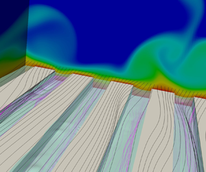
Simulations are performed for a turbulent channel flow with texture on the lower wall (figure 1). The surface textures consist of either longitudinal or transversal bars. The height of the ridges is $k=0.05h$. Three values for pitch $p$ between two consecutive ridges are considered, specifically $p/k = 2,4,8$. The gas fraction (i.e. the ratio of the volume of the cavities to the total volume in the substrate) is kept constant for the different pitch values and equal to $50\,\%$. The computational box is $6.4h\times 2.05h\times 3.2h$ in the streamwise ($x$), wall-normal ($y$) and spanwise ($z$) directions, respectively. The additional $0.05h$ increase in channel height corresponds to the cavity height where the surface textures are placed. Details on the grid resolution are discussed in the appendix. Periodic boundary conditions are applied in the streamwise and spanwise directions. No-slip conditions are imposed on the channel walls. Isothermal boundary conditions are applied on the two walls, with the textured wall at temperature $T^*_w$ and the upper wall at $T^*_u<T^*_w$ (‘$^*$’ denotes dimensional quantities). The temperature in (2.3), and in the remainder of the paper, is normalized as $T=1-2[(T^*-T^*_w)/(T^*_u-T^*_w)]$. Thus, it is equal to $T=1$ on the textured wall, and equal to $T=-1$ on the upper smooth wall. The flow field is initialized with a parabolic velocity profile in the streamwise direction above the crest plane. Disturbances are applied to promote transition to turbulence. The initial temperature profile varies linearly from $T=T_w=1$ at the crest plane to $T=T_u=-1$ at the top wall. In the substrate the temperature is initially uniform at $T=T_w$, and the velocity is zero. No disturbances are applied to the secondary flow in the textures.

Figure 1. Channel configuration: (a) longitudinal bars; (b) transversal bars. The turquoise surface at the crest plane is the interface.

3. Surface performance in ideal conditions: flat interface

The results for the idealised case of infinite surface tension ($We=0$) are presented first. In LIS and SHS the secondary fluid and the substrate texture create heterogeneous solid-fluid and fluid-fluid interfaces at the crest plane. Over the fluid-fluid interface (above the cavities) the primary stream can slip. From a macroscopic point of view, this generates a non-zero ‘effective’ slip length $b$, defined as

(3.1)\begin{equation} \bar{U}_s = b\left.\frac{\textrm{d}\bar{U}}{\textrm{d} y}\right|_{y_w}, \end{equation}

where $\bar {U}_s$ is the apparent ‘slip’ velocity at the crest plane (Lauga, Brenner & Stone Reference Lauga, Brenner and Stone2007); $y_w$ indicates the crest plane and $\textrm {d}\bar {U}/\textrm {d} y$ is the local gradient in the normal direction. The overline denotes an average in time and in the streamwise and spanwise directions. Thus, the slip length is the distance from the crest plane, where the extrapolated velocity profile vanishes. The slip conditions at the interface affect the performance of LIS and SHS, in particular the drag reduction $DR$, defined as

(3.2)\begin{equation} DR = \frac{\tau_0 - \tau}{\tau_0}, \end{equation}

where $\tau$ indicates the surface drag and subscript ‘$0$’ refers to the smooth wall benchmark. The correlation between the amount of drag reduction and the slip length has been widely reported in the literature (Fukagata, Kasagi & Koumoutsakos Reference Fukagata, Kasagi and Koumoutsakos2006; Park et al. Reference Park, Park and Kim2013; Jung, Choi & Kim Reference Jung, Choi and Kim2016; Seo & Mani Reference Seo and Mani2016; Fu et al. Reference Fu, Arenas, Leonardi and Hultmark2017; García Cartagena et al. Reference García Cartagena, Arenas, Bernardini and Leonardi2018; Rastegari & Akhavan Reference Rastegari and Akhavan2015, Reference Rastegari and Akhavan2018; Arenas et al. Reference Arenas, García, Orlandi, Fu, Hultmark and Leonardi2019; Chang et al. Reference Chang, Jung, Choi and Kim2019). Present results, compiled in table 1 and shown in figure 2, corroborate to a large extent this observation. In figure 2 the $DR$ is plotted as a function of the slip length in ‘nominal’ wall units, $b^{+0} = bu_{\tau ,0}/\nu$ (where $u_{\tau ,0}=\sqrt {\tau _0/\rho }$ is the friction velocity of the reference smooth channel). This is done consistently with the analytical model derived by Rastegari & Akhavan (Reference Rastegari and Akhavan2015) (also shown in the figure):

(3.3)\begin{equation} DR = \frac{b^{{+}0}}{b^{{+}0} + \textit{Re}/\textit{Re}_{\tau,0}} + \tilde{g}\left(\varepsilon\right). \end{equation}

Here $\tilde {g}(\varepsilon )$ accounts for the effect of the modification of turbulent structures and secondary motion on drag. Longitudinal bars show a very good agreement with the ‘slip’ term in (3.3) for $b^{+0}\lesssim 5$. For larger values of the slip length, that is, for larger $p/k$, secondary motion in the channel becomes more intense and the amount of drag reduction decreases with respect to the theoretical limit (3.3 with $\tilde {g}\equiv 0$). Transversal textures have a small slip length ($b^+<1$) and are drag increasing ($DR<0$) with respect to the smooth wall.

Table 1. Summary of surface performances for $We=0$. The drag reduction is $DR=1-\tau /\tau _0$, where $\tau$ is the drag of the textured wall (one wall only), $\tau _0$ is the friction for a smooth channel; the heat transfer enhancement is defined as $HTE=q/q_0-1$, where $q$ is the heat flux at the textured surface ($q_0$ is the equivalent value for the smooth channel); $b^+=bu_\tau /\nu$ and $b_\theta ^+$ are the slip lengths in wall units.

Figure 2. Drag reduction for the $We=0$ case as a function of the slip length in ‘nominal’ wall units. Symbols, present simulations: longitudinal bars, $m=0.01$ $\bullet$ and $m=0.4$ ${\blacksquare }$; transversal bars, $m=0.01$ ${\blacktriangle }$ and $m=0.4$ ${\blacktriangledown }$. Lines: (3.3) with $\tilde{g}\equiv 0$.

Analogously to the momentum slip length, the thermal slip length $b_\theta$ can be defined as

(3.4)\begin{equation} T_w - \bar{T}_s ={-} b_\theta\left.\frac{\textrm{d} \bar{T}}{\textrm{d} y}\right|_{y_w}, \end{equation}

where $\bar {T}_s = \bar {T}(y_w)$ is the average temperature at the crest plane. Thus, the thermal slip length is the distance from the crest plane at which the extrapolated temperature profile reaches the ‘no-slip’ isothermal value $T_w$. In analogy with the drag case, a larger $b_\theta$ is expected to be associated with a reduced heat transfer rate, because of the consequent reduced temperature gradient. The relationship between $b_\theta$ and the heat transfer performance can be analytically derived from the energy equation. Following an analogous procedure to Fukagata, Iwamoto & Kasagi (Reference Fukagata, Iwamoto and Kasagi2002), after averaging in time and in the horizontal directions (i.e. in $x$ and $z$ directions), the dimensional form of (2.3) reduces to

(3.5)\begin{equation} \frac{\partial}{\partial y}\left[-\alpha (y)\frac{\partial \bar{T}}{\partial y} + \overline{\theta v}\right] = 0. \end{equation}

The overline denotes the average, $\overline{\theta v}$ are the convective fluxes along the wall-normal direction ($\theta =T(x,y,z,t)-\bar {T}(y)$ and $v=V(x,y,z,t)-\bar {V}(y)$, with $\bar {V}(y)=0$ for continuity), which consist of both the dispersive component (due to texture periodicity) and the turbulent component. Equation (3.5) implies that the total heat flux is constant throughout the channel height. In the case of a flat and slippery interface, where $V=0$, its value, $q$, is equal to the molecular heat flux at the interface, $y=0$. Therefore, after integrating from the crest plane ($y=0$, which is also the interface position) to a generic $y$ in the primary fluid domain:

(3.6)\begin{equation} -\alpha_2\frac{\partial \bar{T}}{\partial y} + \overline{\theta v} = \frac{q}{\rho c_p}. \end{equation}

Here $\rho$ is density and $c_p$ the specific heat. Integration from the crest plane ($y=y_w$, or $y=0$ in the present reference frame) to the top wall ($y=2h$) yields

(3.7)\begin{equation} \alpha_2\left(\bar{T}_s - T_u\right) + \int_0^{2h} \overline{\theta v}\,\textrm{d} y = \frac{{q}}{\rho c_p}{2h}, \end{equation}

where $\bar {T}_s$ is the average temperature at the interface (analogous to the slip velocity) and $T_u$ is the temperature of the upper wall, which is constant because of the isothermal boundary condition. Normalizing the fluxes inside the integral in wall units and using the change of variable $\eta =y/h$, we have

(3.8)\begin{equation} \alpha_2\left(\bar{T}_s - T_u\right) + h\frac{q}{\rho c_p}\int_0^{2} \overline{\theta^+v^+}\,\textrm{d}\eta = \frac{{q}}{\rho c_p}{2h}. \end{equation}

Here, $\overline {\theta ^+ v^+}=\overline {\theta v}{\rho c_p}/q = \overline {\theta v}/(T_\tau u_\tau )$, where $T_\tau =q/\rho {c_p}u_\tau$ is the ‘friction’ temperature. Introducing the Stanton number, $St = q/\rho c_p U_b (T_w-T_u)$, (3.8) reads as

(3.9)\begin{equation} \frac{1}{\textit{Re}\textit{Pr}}\left(\frac{\bar{T}_s - T_u}{T_w-T_u}\right) + St\int_0^{2} \overline{\theta^+v^+}\,\textrm{d}\eta = 2St, \end{equation}

which can be recast as

(3.10)\begin{equation} St = \frac{1}{\textit{Re}\textit{Pr}}\left(1-\frac{T_w-\bar{T}_s}{T_w-T_u}\right)\frac{1}{2-I^+} \end{equation}

with $I^+ = \int _0^2\overline {\theta ^+v^+}\,\textrm {d}\eta$. From the energy balance (3.6) in wall units, it follows that $0<I^+<2$, so that the denominator in (3.10) is positive and does not vanish. Using (3.10), the heat transfer enhancement with respect to a smooth wall ($HTE=St/St_0 - 1$) can be expressed as

(3.11)\begin{align} HTE &={-}\frac{T_w-\bar{T}_s}{T_w-T_u} + \left(1+\frac{T_w-\bar{T}_s}{T_w-T_u}\right)\frac{\varepsilon}{2-I^+},\notag\\ &={-}\frac{T_w-\bar{T}_s}{T_w-T_u} + g_\theta(\varepsilon), \end{align}

where $\varepsilon =I^+-I_0^+$ is the difference in the convective fluxes between the textured surface and the smooth wall. From (3.11), the change in heat transfer can be attributed either to heterogeneity of the temperature distribution at the crest plane (for which $\bar {T}_s\ne T_w$) or to the convection in the overlying fluid. In general, since $\bar {T}_s < T_w$, an increase in heat transfer can be expected only if turbulent convection (that is, the $g_\theta$ contribution) is enhanced.

Equation (3.11) is analogous to the relationship derived by Rastegari & Akhavan (Reference Rastegari and Akhavan2015) for the drag reduction,

(3.12)\begin{equation} DR = \frac{\bar{U}_s}{U_b}+g(\varepsilon), \end{equation}

where $g(\varepsilon )$ is a function that accounts for the difference in the Reynolds stresses $\overline {uv}$ between the textured surface and the smooth wall and has a similar structure to $g_\theta$ in (3.11) (see (2.5) of Rastegari & Akhavan Reference Rastegari and Akhavan2015). By introducing the slip length $b$, (3.12) can be expressed in the form of (3.3). Similarly, using the thermal slip length of (3.4), the Reynolds analogy ($St_0=C_{f,0}/2=\textit {Re}_{\tau ,0}^2/\textit {Re}^2$, where $C_{f,0}=\tau _0/\frac {1}{2}\rho U_b^2$ is the friction coefficient, Kestin & Richardson (Reference Kestin and Richardson1963)) and the identities

(3.13)\begin{gather} T_s^+ = b_\theta^+ \textit{Pr}, \end{gather}

(3.14)\begin{gather}\frac{T_w-\bar{T}_s}{T_w-T_u} = b_\theta^{{+}0}\left( HTE+1\right) \frac{\textit{Re}_{\tau,0}}{\textit{Re}}\textit{Pr}, \end{gather}

(3.11) can be expressed as

(3.15)\begin{equation} HTE={-}\frac{b_\theta^{{+}0}\textit{Pr}}{b_\theta^{{+}0}\textit{Pr} + {\textit{Re}}/{\textit{Re}_{\tau,0}}} + \tilde{g}_\theta(\varepsilon), \end{equation}

where $b_\theta ^{+0}=b_\theta u_{\tau ,0}/\nu$ is the nominal value of thermal slip length in wall units. Here $\tilde {g}_\theta$ accounts for the modifications in the convective fluxes compared to the smooth wall as in (3.11). Equation (3.15) is analogous to (3.3) for the drag reduction.

In figure 3 results from the simulations are compared against the analytical model in (3.15). Only the ‘slip’ contribution is considered in figure 3, i.e. $\tilde {g}_\theta \equiv 0$. In general, there is a relatively larger departure from the model trend compared to figure 2, especially as $b_\theta ^{+0} > 1$. For larger values of the thermal slip lengths, modifications to turbulence and secondary motion becomes significant, which is expected as the textures are larger. This suggests that the thermal balance is more sensitive than momentum transport to the turbulent and secondary motions over the textures. Such different sensitivity can be traced back to the dissimilarity in the momentum and temperature governing equations and boundary conditions. The momentum balance integrated across the channel reads as (Rastegari & Akhavan Reference Rastegari and Akhavan2015):

(3.16)\begin{equation} \frac{6}{\textit{Re}}\left(1 - \frac{\bar{U}_s}{U_b}\right) + 3 C_f \int_0^1 \overline{u^+v^+} \left(1-\eta\right)\textrm{d}\eta = C_f. \end{equation}

The integrals of the fluxes $\overline {uv}$ and $\overline {\theta v}$ contribute to the terms $\tilde {g}$ and $\tilde {g}_\theta$ in the expressions for $DR$ and $HTE$, respectively. However, as shown by (3.9) and (3.16), they are weighted by a different factor, dependent on the distance from the crest plane (i.e. $1-\eta$ for $\overline {uv}$, $1$ for $\overline {\theta v}$). Therefore, even in the presence of similar solutions for the turbulent fluctuations $u$ and $\theta$, a different sensitivity of $HTE$ and $DR$ to the secondary motion could be expected. The weighting factor depends on the channel configuration and the boundary conditions. For instance, Kasagi et al. (Reference Kasagi, Hasegawa, Fukagata and Iwamoto2012) have considered a channel with both smooth walls and different boundary conditions for the temperature field. Following a similar approach to derive (3.9), different weighting factors are obtained for the contribution of the turbulent heat flux to the Stanton number. They suggest this as a possible mean to achieve ‘dissimilar control’ (i.e. simultaneous heat transfer enhancement and drag reduction), and present an application using opposition control through blowing and suction. More in general, a dissimilarity in the change in thermal and momentum performance with respect to the smooth wall is also observed for flow over rough walls. In this case, the drag increases more than the heat transfer (see, e.g. Leonardi et al. Reference Leonardi, Orlandi, Djenidi and Antonia2015). Ultimately, the reason for the different behaviour is that the temperature is a scalar field, while the streamwise velocity is a component of a solenoidal vector field. A departure from similarity can be expected when pressure gradients become important in the flow (as, for example, for rough walls), since there is no counterpart for this mechanism in the energy balance for the temperature dynamics.

Figure 3. Heat transfer enhancement for the $We=0$ as a function of the thermal slip lengths in ‘nominal’ wall units. Symbols, present simulations: longitudinal bars, $m=0.01$ $\bullet$ and $m=0.4$ $\blacksquare$; transversal bars, $m=0.01$ $\blacktriangle$ and $m=0.4$ $\blacktriangledown$. Lines: (3.15) with $\tilde {g}_\theta \equiv 0$.

For a given pitch and texture orientation, SHS and LIS have similar heat transfer performance. The dependence on the surface type is probably mitigated by the assumption of uniform thermal diffusivity across the two fluids ($a = 1$). The residual discrepancy, which is larger for increasing pitch, is to ascribe to the turbulent motion over LIS and SHS. Transversal bars have a larger heat flux compared to longitudinal bars, which is expected since a larger heat flux generally corresponds to a larger drag. However, for all textures, the heat flux is reduced compared to the smooth wall ($HTE<0$), although the magnitude of the decrease remains limited (${\lesssim }10\,\%$).

In the temperature profiles in figure 4, normalized in wall units $T^+ = (T_w - \bar {T})\rho c_p u_\tau /q$, an upward shift in the near-wall region is observed. The shift depends on the ‘slip temperature’ and the profiles in the sublayer collapse when plotted as $T^+-T^+_s$, similarly to the velocity case with scaling $U^+-U_s^+$ (Orlandi, Leonardi & Antonia Reference Orlandi, Leonardi and Antonia2008). From (3.11), the magnitude of the shift $T_s^+$ or, equivalently, its value in physical units, $T_w - \bar {T}_s$ (shown in the inset of figure 4), is a measure of the heat transfer reduction. For a given pitch and viscosity ratio, the shift is larger for transversal bars, even though this texture orientation has superior heat transfer performance than longitudinal ridges. This implies that fluxes $\overline {\theta v}$ compensate for the reduction in the temperature gradient to a larger extent. A notable increase in heat flux is observed in the near-wall region for transversal bars (figure 5). The normalization in wall units is a ratio of the convective heat flux to the total heat flux (Kim & Moin Reference Kim and Moin1987). The near-wall peak contributes for more than $10\,\%$ of the surface heat flux in the case of SHS and slightly less than that for LIS. The enhanced heat flux is not due to changes in the structure of the overlying turbulent flow, but rather to the heterogeneity in the crest plane. Using the triple decomposition (Hussain & Reynolds Reference Hussain and Reynolds1970), one can separate the contributions to the total convective flux ($\overline {\theta v}$) of the random (turbulent) component and the dispersive component (Leonardi et al. Reference Leonardi, Orlandi, Djenidi and Antonia2015):

(3.17)\begin{equation} \overline{\theta v} = {\theta v}_{disp}+\overline{\theta'v'}. \end{equation}

Here $\theta '=T-\langle {T}\rangle$ and angle brackets denote the ensemble average of points at the same relative position within the periodic texture. The dispersive heat flux is $\theta v_{disp}=\overline {\tilde {\theta }\tilde {v}}$, where $\tilde {\theta }=\langle {T}\rangle -\bar {T}$ is the coherent fluctuation, due to the surface texture. As shown in the inset of figure 5, over the crest plane, the flux is mostly due to the dispersive component. The dispersive component is related to heterogeneity in the mean flow and is strongly affected by the texture geometry. In particular, the bar orientation seems a primary factor, with longitudinal bars not presenting a near-wall peak in the dispersive stress distribution. In the outer region the heat flux is carried by the turbulent component, but its distribution is not significantly modified compared to the smooth wall case. This is different than the classic case of rough walls. Leonardi et al. (Reference Leonardi, Orlandi, Djenidi and Antonia2015) have shown that transversal square bars can almost duplicate the smooth wall heat flux for pitch-to-height ratio $p/k\gtrsim 6$. The main contribution to the $HTE$ derives from the turbulent convection due to the wall-normal velocity fluctuations (ejections). For smaller $p/k$, the flow tends to skim over the roughness elements decreasing the probability of ejections, thus achieving about the same heat transfer of the reference smooth wall. This latter flow pattern is similar to the present cases with LIS and SHS. The flat interface damps the wall-normal fluctuations from the substrate reducing the contribution of the turbulent heat convection despite the large pitch-to-height ratios (favourable for heat transfer enhancement).

Figure 4. Mean temperature profile for SHS ($a$) and LIS ($b$): smooth channel; longitudinal ridges, $p/k=2$; longitudinal ridges, $p/k=4$; longitudinal ridges, $p/k=8$; transversal bars, $p/k=2$; transversal bars, $p/k=4$.

Figure 5. Convective heat flux $\overline {\theta ^+v^+}$ for SHS (a) and LIS (b): smooth channel; longitudinal ridges, $p/k=2$; longitudinal ridges, $p/k=4$; longitudinal ridges, $p/k=8$; transversal bars, $p/k=2$; transversal bars, $p/k=4$. The inset in ($a$) shows the decomposition in turbulent component $\overline {\theta 'v'}$ () and dispersive component $\theta v_{disp}$ () of the total heat flux () for SHS transversal bars with $p/k=4$.

Even though the heat flux is marginally reduced, the (normalized) heat flux to drag ratio, $q/\tau$, improves compared to the smooth wall reference, figure 6. For a smooth wall, $q/\tau =1$ owing to the Reynolds analogy (i.e. $St/(C_f/2)=1$, Reynolds Reference Reynolds1961; Kestin & Richardson Reference Kestin and Richardson1963). We note that in practice different parameters may be used to measure the heat transfer efficiency depending on the particular application. Webb (Reference Webb1981) reviews some guidelines and examples to define performance evaluation criteria. In the present case, $q/\tau$ (or, equivalently, $St/(C_f/2)$) is the most suited parameter to compare against the smooth wall and study the Reynolds analogy over SHS and LIS. For LIS and SHS with longitudinal bars, $q/\tau$ is larger than one, meaning that these surfaces transfer heat more efficiently per unit drag. For transversal bars, $q/\tau$ is lower than one, which makes these surfaces similar to drag-increasing rough surfaces, for which also $q/\tau <1$ (for instance, transversal square bars and rods considered in Leonardi et al. (Reference Leonardi, Orlandi, Djenidi and Antonia2015)). However, the efficiency remains quite large ($q/\tau >0.9$) compared to the values achieved by rough walls for the same pitch-to-height ratio. This is due to the damping of wall-normal fluctuations caused by the interface, which decreases the momentum transfer inside the substrate limiting the amount of drag increase (Arenas et al. Reference Arenas, García, Orlandi, Fu, Hultmark and Leonardi2019). Although this also reduces the enhanced turbulent thermal mixing, it appears that the effect is more prominent on the momentum balance rather than on the heat transfer.

Figure 6. Heat transfer to drag ratio as a function of the streamwise slip length $b^+$ ($a$), and comparison between streamwise and thermal slip lengths ($b$). Longitudinal bars, $m=0.01$ $\bullet$ and $m=0.4$ ${\blacksquare }$; transversal bars, $m=0.01$ $\blacktriangle$ and $m=0.4$ $\blacktriangledown$.

The texture orientation seems to be the dominant parameter for the heat transfer efficiency. Using (3.3) and (3.15), it is possible to express the heat transfer efficiency as a function of the slip lengths:

(3.18)\begin{equation} \frac{q}{\tau} = \frac{1+HTE}{1 - DR} = \frac{b^{{+}0} + \textit{Re}/\textit{Re}_{\tau,0}}{b_\theta^{{+}0}\textit{Pr} + \textit{Re}/\textit{Re}_{\tau,0}} +{f}\left(\tilde{g},\tilde{g}_\theta\right). \end{equation}

In (3.18), ${f}$ accounts for the contribution of turbulence and secondary motion to (3.3) and (3.15), that is the terms $\tilde {g}$ and $\tilde {g}_\theta$. In the case of $\textit {Pr}=1$ and neglecting ${f}(\tilde {g},\widetilde {g_\theta })$, (3.18) indicates that the heat transfer efficiency is larger than unity if the streamwise slip length is larger than the thermal slip length, $b/b_\theta >1$. Figure 6(b) compares the value of the slip lengths for the various cases and shows a good agreement with this criterion. Transversal textures, for which $q/\tau <1$, are found above the main diagonal in the figure, thus $b < b_\theta$, while for longitudinal ridges, $b > b_\theta$ and $q/\tau > 1$. Results suggest the existence of a continuous transition from rough surfaces and transversal LIS/SHS ($q/\tau <1$) to the smooth wall ($q/\tau =1$), to longitudinal SHS/LIS ($q/\tau >1$). This is corroborated by the recent study of Arenas et al. (Reference Arenas, García, Orlandi, Fu, Hultmark and Leonardi2019), which establishes a common framework for LIS/SHS smooth and rough walls by identifying a unique scaling for the surface drag reduction or increase.

4. Effect of the interface dynamics

The case of a flat interface between the two fluids is an ideal scenario, which can only be asymptotically approximated with a very high surface tension between the fluids. In reality, the interface deforms causing non-zero wall-normal velocity fluctuations at the crest plane, which are critical for the momentum and thermal transport (Orlandi et al. Reference Orlandi, Leonardi, Tuzi and Antonia2003; Orlandi & Leonardi Reference Orlandi and Leonardi2004). A set of DNS has been performed for $We^+=10^{-3}$ (approximately) using the level-set method to track the deformation of the interface and couple it to the momentum equations, as described in § 2. Table 2 reports the details on the interface deformation (and surface performance). The maximum mean deflection of the interface is computed from the level-set function as

(4.1)\begin{equation} \varDelta_{max} ={-}\max_{x,z}[\langle{\varPhi}\rangle\left(x,y_w,z\right)], \end{equation}

and maximum root-mean-square fluctuation as

(4.2)\begin{equation} \varDelta_{rms} = \max_{x,z}\left[\sqrt{\langle{\phi'\phi'}\rangle\left(x,y_w,z\right)}\right]. \end{equation}

Here, $\varPhi$ is the signed distance function from the interface, $\phi '$ is its fluctuation with respect to the phase average (denoted by the angle brackets, $\phi ' = \varPhi - \langle {\varPhi }\rangle$); $y_w$ indicates the crest plane. Therefore, $\varPhi (x,y_w,z)$ quantifies the deflection of the interface from its initial position (flat interface at $y=y_w$). According to the definition of $\varPhi$, a positive value ($\varPhi (x,y_w,z)>0$) indicates that the interface is displaced downward (hence, the minus sign in (4.1) for a more intuitive definition of the sign of the displacement). As expected, the mean deformation and its fluctuation increase with $p/k$. This is consistent with the recent analysis of García Cartagena et al. (Reference García Cartagena, Arenas, An and Leonardi2019). They have shown that, for a substrate made of randomly disposed pinnacles, the mean interface displacement scales roughly linearly with the distance among the points where the interface is pinned (this would be equivalent to the cavity width for a texture of regularly placed bars as considered herein). In the present cases, the maximum displacement is ${\sim } 1$ wall unit for cavity widths $p^+ \approx 18\text {--}36$, which is in close agreement with the magnitude reported by García Cartagena et al. (Reference García Cartagena, Arenas, An and Leonardi2019) for the same Reynolds and Weber numbers ($\varDelta ^+_{max}\approx 1.5$ for widths of about $40$ wall units).

Table 2. Summary of surface performances for $We^+=\mu _2 u_\tau /\sigma \simeq 10^{-3}$; $\varDelta _{max}$ and $\varDelta _{rms}$ are, respectively, the maximum mean and root-mean-square deflection of the interface, computed from the level-set function as $\varDelta _{max} =-\max_{x,z}{[\langle {\varPhi }\rangle (x,y_w,z)]}$, and $\varDelta _{rms} = \max_{x,z}{[\sqrt {\langle {\phi '\phi '}\rangle (x,y_w,z)}]}$. A negative value of $\varDelta _{max}$ indicates a downward displacement of the interface (towards the bottom of the cavity).

Figure 7 shows the $DR$ as a function of the streamwise slip length (defined as in (3.1)). Results for $We^+=10^{-3}$ are represented as empty symbols connected to the corresponding flat interface case to show the effect of the transition to a finite value of surface tension.

Figure 7. Drag reduction as a function of the slip length in ‘nominal’ wall units: longitudinal bars, $m=0.01$ $\bullet$ and $m=0.4$ ${\blacksquare }$; transversal bars, $m=0.01$ $\blacktriangle$ and $m=0.4$ $\blacktriangledown$. Solid symbols, $We=0$; empty symbols, $We^+ = 10^{-3}$. Solid line, (3.3).

The effect on $DR$ is quite different depending on the viscosity ratio. For SHS longitudinal bars, there is a considerable decline in the amount of $DR$. For the shortest pitch ($p/k=2$), the surface generates essentially the same drag of the smooth wall, while for $p/k=4$, more than half of $DR$ amount is lost. Instead, LIS bars are not strongly affected by the change in the surface tension and maintain approximately the same amount of $DR$ as in the ideal case. The interface of LIS is more robust to the overlying coherent structures and pressure fluctuations than SHS. Figure 8 shows the mean velocity profile for super-hydrophobic and liquid-infused longitudinal bars with $p/k=4$ in the cases $We=0$ and $We^+=10^{-3}$. Even in the case of $We=0$, the velocity profiles for LIS and SHS in the cavity are qualitatively different. In these cases the flow in the cavity is mostly driven by the shear of the main fluid, and the velocity profiles show characteristics of shear-driven flows (other textures may result in a pressure-driven flow). Consistently, the velocity profile for LIS can be approximated with a linear velocity profile typical of a laminar Couette flow. For SHS, the motion in the cavity is mostly shear-driven as well, but in this case the profile assumes the shape of a turbulent Couette flow. Since the secondary fluid for SHS is less viscous, the cavity Reynolds number is larger than in the case of LIS. For the texture in the figure ($m=0.01, p/k=4, We=0$), the Reynolds number for the flow in the cavity is

(4.3)\begin{equation} \textit{Re}_{cav} = \frac{\rho\,\bar{U}_s k}{4 \mu_1} \approx 600. \end{equation}

Here, the Reynolds number is defined as normally done for Couette flows with $k/2$ and half the velocity difference $\bar {U}_s/2$ (see the inset in figure 8 for the definitions). The value is larger than the transitional Reynolds number for which turbulence can be sustained in a Couette flow ($\textit {Re}_{trans} = 360$; see e.g. Lundbladh & Johansson Reference Lundbladh and Johansson1991; Tillmark & Alfredsson Reference Tillmark and Alfredsson1992; Komminaho, Lundbladh & Johansson Reference Komminaho, Lundbladh and Johansson1996). Figure 9 shows second-order turbulence statistics in the cavity. Results are devoid of the dispersive component and normalized with a cavity friction velocity:

(4.4)\begin{equation} u_{\tau,c} = \sqrt{\frac{\tau_c}{\rho}} = \sqrt{\frac{1}{\rho}\mu_1 \left.\frac{\textrm{d}\bar{U}}{\textrm{d} y}\right|_{y ={-}k}}. \end{equation}

The side walls are not included in the definition of $u_{\tau ,c}$, because, as suggested by studies in duct flows (Gavrilakis Reference Gavrilakis1992; Vinuesa et al. Reference Vinuesa, Noorani, Lozano-Durán, El Khoury, Schlatter, Fischer and Nagib2014; Pirozzoli et al. Reference Pirozzoli, Modesti, Orlandi and Grasso2018; Orlandi & Pirozzoli Reference Orlandi and Pirozzoli2020a,Reference Orlandi and Pirozzolib), the ‘local’ friction (as opposed to the total friction) is the appropriate scaling for one-point turbulence statistics (we remind the reader that this is related to the analysis of the cavity and the definition of $u_{\tau ,c}$ only; the friction on all walls is considered in the overall $u_\tau$ for the surface used in the preceding and following sections). The velocity fluctuations are consistent with the typical behaviour of Couette flow turbulence in the lower half of the cavity ($y/k<-0.5$). Approaching the crest plane ($y/k=0$), the streamwise and spanwise components do not vanish, as it would occur for a physical wall, owing to the variations of the velocity at the interface and the overlying flow turbulence. Instead, the wall-normal component tends to zero as expected, because $V(\kern-0.05em y/k=0)\equiv 0$ at the interface for $We=0$. The Reynolds shear stress $\overline {u'v'}$ (figure 9b) shows the constant trend in the middle of the cavity typical of the turbulent Couette flow. The value in wall units is not closer to unity probably because of the presence of the side walls (which accounts for part of the friction). The results for the smaller cavity ($p/k=2$) are also consistent with Couette flow turbulence. In this case the cavity Reynolds number is about the same as the transitional value ($\textit {Re}_{cav} \approx 360$), and low-Reynolds effects are visible, for example, in the Reynolds shear stress distribution. At any rate, the intensity of this turbulent motion inside the cavity is low compared to the turbulence intensity in the main stream. The frictional Reynolds number $\textit {Re}_{\tau ,c} = \rho u_{\tau ,c} (k/2)/\mu _1$ for the flow in the cavity is about $50$ and $70$ for $p/k=2$ and $p/k=4$, respectively. In the case of LIS the cavity Reynolds number $\textit {Re}_{cav} = \rho \bar {U}_s k/4\mu _1 \approx 10$ is well below the transitional Reynolds number and the velocity in the cavity is closer to the laminar linear profile.

Figure 8. Mean velocity $\bar {U}$ profile near the interface ($y/h=0$) for longitudinal ridges with $p/k=4$. Super-hydrophobic surfaces ($m=0.01$): $\,We=0$; $\,We^+=10^{-3}$. Liquid-infused surfaces ($m=0.4$): $We=0$; $We^+=10^{-3}$. Smooth channel case: .

Figure 9. Turbulence statistics in the cavity for SHS longitudinal bars with $p/k = 4$ (black lines) and $p/k=2$ (red lines). (a) Root-mean-square velocity fluctuations: $u^{+c}_{rms} = \overline {u'u'}^{1/2}/u_{\tau ,c}$; $v^{+c}_{rms} = \overline {v'v'}^{1/2}/u_{\tau ,c}$; $w^{+c}_{rms} = \overline {w'w'}^{1/2}/u_{\tau ,c}$. (b) Reynolds shear stress $-\overline {u'v'}$.

With the variation in surface tension, the velocity profile for LIS is largely unaltered apart from minor changes in the neighbourhood of the crest plane ($y/h=0$). Conversely, in the case of super-hydrophobic surfaces, the velocity inside the cavity ($y/h<0$) increases considerably for $We^+=10^{-3}$. When the interface deforms ($We^+=10^{-3}$), more momentum is transferred (and dissipated) inside the cavities by the Reynolds stress $\overline {uv}$ at the interface, which decreases the amount of $DR$ (Arenas et al. Reference Arenas, García, Orlandi, Fu, Hultmark and Leonardi2019). The momentum balance in the cavity for super-hydrophobic and liquid-infused surfaces has been analysed in detail by Arenas et al. (Reference Arenas, García, Orlandi, Fu, Hultmark and Leonardi2019). The conditions at the interface determine the drag in the cavity, as they have shown integrating the momentum (2.2) over the volume of the cavity:

(4.5)\begin{equation} \int_{S_{int}} \left[\frac{1}{\textit{Re}} \frac{\textrm{d}\langle{U}\rangle}{\textrm{d} y} - \langle{u v}\rangle\right] \textrm{d}S + \langle{\varPi}\rangle V_t = \int_{S_{cav}} \frac{m}{\textit{Re}} \frac{\textrm{d}\langle{U}\rangle}{\textrm{d} n} \textrm{d}S. \end{equation}

Here $S_{int}$ is the surface of the interface between the two fluids, $S_{cav}$ is the surface of the cavity and $V_t$ is the volume of the cavity. The drag in the cavity, i.e. the right-hand side of the equation, has no form drag component for the case of longitudinal bars. Equation (4.5) is applicable also for $We\ne 0$ if the interface deformation is small, which is appropriate for the present textures (table 2). Figure 10 shows the viscous and Reynolds shear stresses for SHS and LIS longitudinal bars with $p/k=4$. Following (4.5), the stresses are averaged over the interface (denoted with the overline and superscript $i$). For SHS, in the case of $We^+=10^{-3}$ both the viscous stress and the Reynolds stress increase compared to the flat interface case. This increases the shear-driven momentum in the cavity, and eventually the drag as quantified by (4.5). In the case of LIS the discrepancy between the $We^+=0$ and $We^+=10^{-3}$ cases is negligible and, consistently, the profiles in figure 8 essentially collapse onto each other.

Figure 10. Shear stress balance for longitudinal bars, with $p/k=4$ and $m=0.01$ (a, SHS) and $m=0.4$ (b, LIS). Lines are for the viscous shear stress, symbols (plotted every $4$ points, for clarity) are for the Reynolds stress $\langle {uv}\rangle$. Solid lines and symbols (, $\blacksquare$) denote $We = 0$ cases, dashed lines and empty symbols (, $\square$) are for the $We^+= 10^{-3}$ cases.

For transversal bars, the finite surface tension slightly reduces the yet modest streamwise slip length. The drag is also marginally affected, except for the SHS case with the largest pitch-to-height ratio ($p/k=4$), for which drag is increased. This case approaches to the rough wall scenario, where, for large $p/k$ values, strong $\overline {uv}$ events contribute to intensify and maximize drag increase (Leonardi et al. Reference Leonardi, Orlandi, Smalley, Djenidi and Antonia2003).

The effect on the heat transfer enhancement and thermal slip length is shown in figure 11(a). The thermal slip length tends to be smaller than one viscous unit ($b_\theta ^{+0}\lesssim 1$, see also table 2) for transversal bars, while it does not significantly change for longitudinal bars. A general increase in the heat flux is observed. For SHS textures, particularly, this is sufficient to achieve a positive $HTE$, meaning that the surface sustains a larger heat flux than the smooth wall, whereas in the ideal flat interface scenario $HTE<0$ for all surfaces. The main mechanism for the performance enhancement is the generation of $\overline {\theta v}$ flux at the interface. Figure 11(b) shows as an example the convective flux and the mean temperature profile (inset) for one case with $HTE>0$. The mean profile $\bar {T}$ is not significantly changed following the variation in Weber number, particularly the gradient at the interface, which determines the molecular heat flux. However, for $We^+\ne 0$, the total heat flux is the sum of the molecular heat flux and the convective contribution, which does not vanish as for the infinite surface tension case. This is evident from the $\overline {\theta v}$ profile. The enhancement in the convective flux is mainly due to the turbulent heat flux (shown with the grey thick line in figure 11b). The dynamics of the interface allows the generation of wall-normal fluctuations and turbulent transport at the crest plane, whereas this mechanism is damped when $We=0$.

Figure 11. (a) Heat transfer enhancement as a function of $b_\theta ^{+0}$: longitudinal bars, $m=0.01$ $\bullet$ and $m=0.4$ ${\blacksquare }$; transversal bars, $m=0.01$ $\blacktriangle$ and $m=0.4$ $\blacktriangledown$. Solid symbols, $We=0$; empty symbols, $We^+ = 10^{-3}$. Solid line, (3.15). (b) Total convective heat flux $\overline {\theta ^+ v^+}$ for SHS longitudinal ridges with $p/k=4$, $m=0.01$: $We=0$; $We^+=10^{-3}$; smooth channel. The grey thick line (, grey) shows the turbulent component $\overline {\theta 'v'}$ for the $We^+=10^{-3}$ case. The inset shows the mean temperature profile $\bar {T}$ near the substrate.

The turbulent heat flux $\langle {\theta 'v'}\rangle$ is also visualized in figure 12 for longitudinal bars with $p/k = 4$. Super-imposed vorticity contours indicate the presence of counter-rotating vortex pairs. This flow pattern over longitudinal SHS/LIS has been documented by Arenas et al. (Reference Arenas, García, Orlandi, Fu, Hultmark and Leonardi2019), which have compared it to the analogous flow structures observed at the tip of riblets. Longitudinal streamwise vortices, also generated over ribbed channels, are beneficial for heat transfer improvement (Hetsroni et al. Reference Hetsroni, Mosyak, Rozenblit and Yarin1999; Miyake et al. Reference Miyake, Tsujimoto and Nakaji2001; Leonardi et al. Reference Leonardi, Orlandi, Djenidi and Antonia2004). The intensity of the vortices is larger for SHS than LIS. In addition, the vortical motion in the cavities is stronger for SHS, which is a consequence of the local turbulent motion for this texture. With $We^+=10^{-3}$, the vortices intensify and the downwash in the middle of the cavity induces a mean downward displacement of the interface. This secondary motion affects the distribution of $\langle {\theta 'v'}\rangle$, and results in a clear increase of the turbulent heat flux for $m=0.01$. In fact, this texture has a $HTE>0$. Transversal bars present a much weaker secondary motion and are not shown here.

Figure 12. Turbulent heat flux $\langle {\theta 'v'}\rangle$ with superimposed streamwise vorticity $\langle {\varOmega _x}\rangle$ contours () for longitudinal bars with $p/k=4$. Top row (a,b): $m = 0.01$ (SHS); bottom row (c,d): $m=0.4$ (LIS). Left (a,c), $We = 0$; right (b,d), $We^+ = 10^{-3}$. Contour lines every $0.025$ for SHS, and every $0.015$ for LIS. The thick red line denotes the mean interface position.

As a result of the interface deformation and the increased fluxes at the crest plane, the correlation between $HTE$ and $b_\theta$ is almost lost. This is the case also for drag reduction and streamwise slip length (figure 7). The common reason is that, in the presence of a deformable interface, the slip conditions at the interface are no longer the sole or dominant factor for either drag reduction or heat transfer enhancement. Wall-normal velocity fluctuations lead to the generation of Reynolds shear stresses $\overline {uv}$ and fluxes $\overline {\theta v}$. The terms $\tilde {g}$ and $\tilde {g}_\theta$ in (3.3) and (3.15) acquire increasing importance, which leads to the departure from the pure ‘slip’ behaviour.

The heat transfer efficiency $q/\tau$ and the slip length comparison for the $We^+=10^{-3}$ cases are shown in figure 13. For transversal bars, the ratio $b/b_\theta$ tends to the main diagonal, $b = b_\theta$. Consistently with (3.18), the heat transfer efficiency for these textures tends to the smooth wall value, $q/\tau =1$. Analogously, $q/\tau$ is generally increased, and remains above $1$, for the cases with longitudinal orientation, for which $b > b_\theta$. Thus, the results for the deformable interface case have a good agreement with (3.18), although this expression was derived neglecting turbulent and secondary motions in the channel. These motions become more important for finite surface tension (see, for example, the departure from the analytical trends in figures 2 and 3). However, since their effect is to increase (with respect to the $We=0$ case) both $q$ and $\tau$ (figures 7 and 11), their impact on the ratio $q/\tau$ approximately cancels out.

Figure 13. Heat transfer to drag ratio as a function of the streamwise slip length $b^{+0}$ (a), and comparison between streamwise and thermal slip lengths (b). Longitudinal bars, $m=0.01$ $\bullet$ and $m=0.4$ ${\blacksquare }$; transversal bars, $m=0.01$ $\blacktriangle$ and $m=0.4$ $\blacktriangledown$. Solid symbols, $We=0$; empty symbols, $We^+ = 10^{-3}$.

Compared to the ideal flat interface case, the efficiency is improved for essentially all the geometries. In particular, SHS longitudinal textures achieve $q/\tau >1$ by simultaneously reducing drag and increasing the heat transfer rate. This leads to an apparent breakdown of the Reynolds analogy, understood in a broad sense as the inevitable correlation between heat transfer enhancement and drag increase. In reality, this is justified by the original lack of similarity between the thermal and momentum balance in the governing equations (2.2) and (2.3). With respect to the classical case (Teitel & Antonia Reference Teitel and Antonia1993), the different properties of the two fluids and the presence of the interface between them are reflected in a different way in the balance equations. In addition, the textured two-fluid configuration of LIS and SHS involves additional sources of energy-momentum dissimilarity. The surface tension force $f_i$ in (2.2) has no counterpart in the energy equation. Likewise the pressure term, which may be significant in the substrate (Arenas et al. Reference Arenas, García, Orlandi, Fu, Hultmark and Leonardi2019), affects only the momentum equation. In summary, the physical mechanisms involved in non-canonical wall-bounded flows such as LIS and SHS provide novel potential for so-called ‘dissimilar control’ (Hasegawa & Kasagi Reference Hasegawa and Kasagi2011; Kasagi et al. Reference Kasagi, Hasegawa, Fukagata and Iwamoto2012), i.e. the simultaneous drag reduction and heat transfer increase.

5. Effect of fluid properties

Different viscosity and/or diffusivity ratios $a$ and $m$ will affect the transport mechanisms over the surface, changing the thermal and momentum balance. In this section we analyse the sensitivity to the fluid properties of the surface performance. Table 3 summarizes the cases considered for this parametric study.

Table 3. Parametric study on fluid properties: summary of surface performance. The ‘riblets’ case indicates longitudinal bars with $p/k=2$ and one fluid only. The heat transfer statistics for $\textit {Pr}=7$ cases are computed with respect to a smooth channel with one fluid and $\textit {Pr}=7$.

In terms of drag reduction, Fu et al. (Reference Fu, Arenas, Leonardi and Hultmark2017) have analysed to a great extent its dependence upon the viscosity ratio $m$ in the case of $We=0$, noting that $DR>0$ even for $m\approx {O}(1)$. As recently clarified by Arenas et al. (Reference Arenas, García, Orlandi, Fu, Hultmark and Leonardi2019), the interface enables $DR$ even when the infused liquid has a viscosity of the same order of the primary fluid, by suppressing wall-normal velocity fluctuations. Present results for $m=1$ and $We=0$ are consistent with these previous studies (figure 14). In addition, the $DR$ is larger than what is obtained when the same texture (longitudinal bars with $p/k = 2$) is wet by the primary fluid only. As explained by Arenas et al. (Reference Arenas, García, Orlandi, Fu, Hultmark and Leonardi2019), this is due to the interface, which avoids the typical failure mechanism of riblets with the secondary streamwise vortices (such as those in figure 12) penetrating inside the cavities. The deformation of the interface ($We^+ = 10^{-3}$ case) does not change much the drag reduction performance. As explained above comparing LIS ($m = 0.4$) and SHS ($m = 0.01$), a large viscosity of the fluid in the cavity damps the momentum transfer from the primary fluid and avoids the generation of strong wall-normal velocity fluctuations, which would reduce the amount of $DR$. The thermal performance is also very similar among these textures and scales well with the thermal slip length (figure 14b). The observed reduction in heat flux for ‘riblets’ corroborates findings from previous studies (Stalio & Nobile Reference Stalio and Nobile2003; Orlandi et al. Reference Orlandi, Sassun and Leonardi2016).

Figure 14. Drag reduction (a) and heat transfer enhancement (b) as a function of the slip lengths ($b$ and $b_\theta$, respectively) in ‘nominal’ wall units for longitudinal bars. Symbols (as in figure 2): $m=0.01$ $\bullet$ and $m=0.4$ ${\blacksquare }$. Additional cases in table 3: $m=1$ ${\blacklozenge }$ (green) (solid, $We=0$; empty, $We^+=10^{-3}$); ‘riblets’ ${\blacklozenge }$ (black). Red symbols (${\blacksquare , \bullet }$) denote the change in diffusivity ratio $a$: solid symbols, $\textit {Pr} = 1$; half-solid, $\textit {Pr} = 7$. Lines: (a) (3.3) with $\tilde {g}\equiv 0$; (b) equation (3.15) with $\tilde {g}_\theta \equiv 0$ and $\textit {Pr}=1$; (3.15) with $\tilde {g}_\theta \equiv 0$ and $\textit {Pr}=7$.

As it could be expected, the $HTE$ is more sensitive to the variation in the thermal diffusivity ratio $a=\alpha _1/\alpha _2$, rather than the diffusivity ratio. Two values of $a$ have been considered, $a=0.04$ and $a=0.23$, to mimic the conductivity ratio of water over air and water over heptane, respectively. With the reduction in the thermal diffusivity of the secondary fluid, compared to reference case $a=1$, the heat flux carried in the cavity decreases. This results in larger thermal slip length $b_\theta$ and lower slip temperature $\bar {T}_s$. The total heat transfer rate decreases by about $10\,\%$, especially for SHS ($m=0.01$) because of the low thermal conductivity. The decrease in $HTE$ is consistent with (3.15), although the contribution of turbulence and secondary motion in the overlying channel is larger than for the same geometry ($p/k=4$) and $a=1$. This can be expected since the larger heterogeneity at crest plane (i.e. larger $T_w - \bar {T}_s$) leads to a larger dispersive flux partly compensating for the reduction in molecular heat flux in the cavity.

According to (3.15), an increase in the Prandtl number of the primary fluid ($\textit {Pr}=\nu _2/\alpha _2$) leads to a comparatively larger downgrade in $HTE$ compared to the unitary Prandtl number case for a given thermal slip length. Two simulations have been performed for $\textit {Pr} = 7$, which is approximately the value for water as a working fluid. The value of $HTE$ is effectively reduced for both LIS and SHS. However, the reduction compared to the smooth wall is significantly less than what would be predicted by the slip contribution only. The thickness of the thermal boundary layer reduces for high-$\textit {Pr}$ fluids, and near-wall turbulent coherent structures can mix fluid in a layer with low thermal resistance. Therefore, the importance of turbulent convection increases, which explains the larger discrepancy from the slip trend of (3.15).

In addition, the SHS texture ($m=0.01$, $\textit {Pr} = 7$) yields a larger heat flux than the LIS case, despite the fluid in the cavity having a much lower diffusivity. Turbulent heat transport ($\overline {\theta v}$) also occurs in the cavity for this texture. Figure 15(a) shows the mean temperature profile for the $\textit {Pr} = 7$ simulations, which present a similar trend to the velocity profiles in figure 8. Because of the larger Prandtl number of the fluid in the cavity ($\textit {Pr}_1 = \nu _1/\alpha _1 = \textit {Pr}\, m/a$), the temperature profile also assumes a characteristic turbulent shape (as opposed to the inset in figure 11b). Owing to the additional turbulent contribution, the fluid in the cavity is able to carry a larger heat flux than with conduction only. In that case, the heat flux in non-dimensional form could be expressed as

(5.1)\begin{equation} q = \frac{a}{\textit{Re}\textit{Pr}} \frac{T_w - \bar{T}_s}{k}, \end{equation}

with $k$ being the cavity height. Figure 15(b) shows that all textures follow with a close approximation (5.1). The data points lie below the curve because (5.1) does not account for the lateral walls in the cavity, but is just based on one-dimensional conduction. The only exceptions to this trend are represented by the SHS textures with $a=0.04$, and notably for the $\textit {Pr} = 7$ case (the $\textit {Pr}=1$ case also presents a moderate turbulent ‘S’-profile).

Figure 15. (a) Temperature profile for the $\textit {Pr} = 7$ cases near the crest plane ($y/h = 0$): smooth wall; $m=0.4$ and $a=0.23$ (LIS); $m=0.01$ and $a=0.04$ (SHS). (b) Non-dimensional heat flux as a function of $T_w - \bar {T}_s$ for all the $We = 0$ cases with longitudinal bars. Solid symbols denote LIS textures ($m=0.4$), empty symbols are for SHS ($m=0.01$). Diffusivity ratios: $a=1~\blacksquare$; $a=0.23$ $\bullet$; $a=0.04$ $\blacktriangle$. The case $m=1$ and $a=1$ is denoted with ${\blacklozenge }$ (green). Lines: (5.1) with $a=1$ (); $a=0.23$ (); $a=0.04$ ().

Figure 16 shows the heat transfer efficiency. The results are presented as $(q/q_0)\cdot (\tau _0/\tau )$ because for $\textit {Pr} = 7$ the non-dimensional heat flux to drag ratio is $q/\tau \approx 0.3$, in fairly good agreement with the Colburn analogy factor ($q/\tau =2 St / C_f =\textit {Pr}^{-2/3}$; Colburn Reference Colburn1964). The case $m=1$ is close to the LIS texture with the same geometry ($p/k$) both for $We=0$ and $We=10^{-3}$, which is consistent with the general trends discussed in §§ 3 and 4, for textures with high-viscosity secondary fluid. For the values considered in this study, the variation in the diffusivity ratio $a$ tends to reduce the heat flux to drag ratio. This is because the drag is not affected by the value of $a$, since the temperature is treated as a passive scalar (in fact, the textures have, approximately, the same drag and slip length for different values of $a$). On the other hand, the heat transfer rate is reduced because of the reduced thermal capacity in the cavities. Figure 16(b) supports to a good approximation the correlation derived in (3.18) between $b/b_\theta > 1$ and $q/\tau > 1$.

Figure 16. Heat transfer to drag ratio as a function of the streamwise slip length $b^{+0}$ ($a$), and comparison between streamwise and thermal slip lengths ($b$). Symbols as in figure 14.