


1. INTRODUCTION
Software-defined radio technology is generating widespread interest in Global Navigation Satellite System (GNSS) receivers. Designers can develop and verify signal processing algorithms on a flexible open-architecture (Borre and Akos, Reference Borre and Akos2005). To facilitate algorithm design, an Intermediate Frequency (IF) GNSS signal usually serves as the signal source for a software receiver. Thus, the IF signal quality has a direct impact on the performance evaluation of signal processing algorithms, such as GNSS signal tracking. A high-quality GNSS IF signal simulator should take into account the error sources from both the satellite vehicles and the receiver. This paper focuses on the latter. Specifically, the phase noise of a receiver's internal oscillator is considered when simulating the IF signal.
High-end oscillators, such as very stable Oven Controlled Crystal Oscillators (OCXOs), caesium and rubidium atomic oscillators, and the recently developed chip-scale atomic clocks, have proved to exhibit high performance in various aspects of GNSS receivers (Weinbach and Schön, Reference Weinbach and Schön2011; Yeh et al., Reference Yeh, Chen, Xu, Wang and Chen2013; Gowdayyanadoddi et al., Reference Gowdayyanadoddi, Broumandan, Curran and Lachapelle2014; Krawinkel and Schön, Reference Krawinkel and Schön2015). Most receivers, however, use Temperature Compensated Crystal Oscillators (TCXOs) as their frequency reference. The low-cost TCXOs exhibit more serious Allan Deviation (ADEV) phase noise compared with the above-mentioned high-end oscillators. The ADEV phase noise poses a threat to the performance of a GNSS receiver, because the phase noise manifests itself in the form of signal dynamics, and the tracking loop bandwidth has to be increased to avoid loss of lock due to the oscillator-induced frequency fluctuations (Curran et al., Reference Curran, Lachapelle and Murphy2012). The phase jitter induced by the ADEV phase noise is also an error source of the Phase Lock Loop (PLL) measurement (Irsigler and Eissfeller, Reference Irsigler and Eissfeller2002; Razavi et al., Reference Razavi, Gebre-Egziabher and Akos2008; Wang and Li, Reference Wang and Li2012).
A software receiver suffers more from oscillator-induced frequency variations than a hardware correlator-based receiver, because a software receiver generates its local carrier assuming a nominal frequency (Kou et al., Reference Kou, Jiao and Morton2011; Kou and Morton, Reference Kou and Morton2013). Typically, the receiver's Radio Frequency (RF) part and the baseband part share one frequency reference. The oscillator-induced frequency fluctuations are amplified proportionally, when generating the local carrier. Take a Global Positioning System (GPS) L1 receiver for example. A 10 MHz TCXO is used as the frequency reference for both the RF and baseband part. A local carrier at 1,575 MHz is generated to mix the RF signal into the IF signal. A frequency variation of approximately 0·1 Hz in the TCXO would result in a 15·75 Hz frequency deviation in the RF carrier, as well as in the digitised IF signal. This frequency deviation would be an obstacle to overcome for a software receiver, especially for the carrier phase tracking process. Thus, to provide the software receiver with a high-fidelity test environment, an IF signal simulator must consider these oscillator-induced frequency fluctuations.
The remainder of this paper is organised as follows. In the next section, the theory of oscillator phase noise is briefly introduced, including the concept of power-law spectral density and the ADEV. Section 3 presents the IF signal simulation method, where a pseudolite transmitter and receiver system is developed to measure the parameters of the receiver's oscillator. In Section 4, performance of the developed measurement system is assessed, and the oscillator's effect on the PLL performance of a software receiver is analysed in detail. Section 5 concludes the paper.
2. OSCILLATOR PHASE NOISE CHARACTERISATION
The oscillator phase process Φ(t) is expressed as (Lindsey and Chie, Reference Lindsey and Chie1976):
 $$\Phi(t) = 2\pi v_{0}t + \sum^{N}_{k=2} \displaystyle{{2\pi\delta v_{k-1}}\over{k!}} t^{k} + \phi(t)$$
 where ν0 and δνk are the oscillator's constant mean frequency and the kth-order frequency drifts, respectively. The second term  $\sum\limits^{N}_{k=2}\displaystyle{{2\pi\delta v_{k-1}}\over{k!}} t^{k}$ represents the long-term phase drift process, which poses no threat to a GNSS carrier tracking loop, as any frequency bias can be absorbed into the Doppler estimate. The higher order frequency drifts are negligible (Curran et al., Reference Curran, Lachapelle and Murphy2012). Thus, the long-term effects are neglected. The last term ϕ(t) is the random phase fluctuation, which may be expressed as the instantaneous normalised (or fractional) frequency fluctuations y(t) by using the relationship:
 $$y(t) = \displaystyle{{1}\over{2\pi v_{0}}} \displaystyle{{\hbox{d}\phi(t)}\over{\hbox{d}t}}$$
The power spectral density S y(f) of y(t) is defined as (Vernotte et al., Reference Vernotte, Lantz, Groslambert and Gagnepain1993):
 $$S_{y}(f) = \hbox{FT} \left[{\int^{+\infty}_{-\infty}y(\theta)y(\theta-t)\hbox{d}\theta}\right]$$
where FT[.] represents the Fourier transform operation. For most frequency sources, S y(f) can be approximated by the sum of five independent noise processes (Barnes et al., Reference Barnes, Chi, Cutler, Healey, Leeson, Mcgunigal, Mullen, Smith, Sydnor, Vessot and Winkler1971), as
 $$S_y(f) = \left\{ {\matrix{ {\sum\limits_{\alpha = - 2}^{ + 2} {h_\alpha } f^a} \hfill & {0 \le f \le f_h} \hfill \cr 0 \hfill & {f \gt f_h} \hfill \cr } } \right.$$
where f is the Fourier frequency in Hertz. The coefficients h α represent the intensity of five noise processes: Random Walk Frequency Modulation (RWFM, α = −2), Flicker Frequency Modulation (FFM, α = −1), White Frequency Modulation (WFM, α = 0), Flicker Phase Modulation (FPM, α = 1) and White Phase Modulation (WPM, α = 2). The term f h is the high-frequency cut-off of the measuring system in Hertz.
An oscillator's short-term stability can also be described in the time domain by the non-overlapped or two-sample ADEV (Allan, Reference Allan1987):
 $$\sigma_{y}(\tau) = \left[\displaystyle{{1}\over{2(M-1)}} \sum^{M-1}_{k=1}(\bar{y}_{k+1} - \bar{y}_{k})^{2}\right]^{1/2}$$
where ȳ k is the kth of M fractional frequency values averaged over the measurement interval, τ. The overlapped ADEV, which improves the confidence of a stability estimate, is calculated by the expression (Riley, Reference Riley2008):
 $$\sigma_{y}(\tau) = \left[\displaystyle{{1}\over{2m^{2}(M-2m+1)}} \sum^{M-2m+1}_{j=1}\left(\sum^{j+m-1}_{k=j}(\bar{y}_{k+m} - \bar{y}_{k})\right)^{2}\right]^{1/2}$$
where m is called the averaging factor.
The relationship between the time and frequency domain description of an oscillator's frequency stability is (Vernotte et al., Reference Vernotte, Lantz, Groslambert and Gagnepain1993):
 $$\sigma_{y}(\tau) = \left[2\int^{f_{h}}_{0}S_{y}(f)\displaystyle{{\sin^{4}(\pi \tau f)}\over{(\pi \tau f)^{2}}}\hbox{d}f\right]^{1/2}$$
Based on a power law noise model for the noise processes involved, time and frequency domain conversions may be made by use of a numerical approximation as follows (Riley, Reference Riley2008):
 $$\sigma_{y}(\tau) = \left[h_{-2}\displaystyle{{(2\pi)^{2}}\over{6}} \tau + h_{-1}2\hbox{ln}\, 2 + h_{0} \displaystyle{{1}\over{2\tau}} + h_{1} \displaystyle{{1.038+3 \hbox{ln}(2\pi f_{h} \tau)}\over{(2\pi)^{2}\tau^{2}}} + h_{2} \displaystyle{{3f_{h}}\over{(2\pi)^{2}\tau^{2}}}\right]^{1/2}$$
It should be noted that the type of noise that dominates an oscillator's performance depends on the averaging interval of the measuring system or on the particular range of Fourier frequencies in the frequency domain. Figure 1 is a log-log plot of the ADEV of a typical TCXO with h-parameters as follows: h −2 = 2 · 4e − 22, h −1 − 2·4e − 21, h 0 = 3·9e − 22, h 1 = 2·5e −23 and h 2 = 2·0e −26 (Curran et al., Reference Curran, Lachapelle and Murphy2012). The slope characteristics are also plotted. Table 1 shows the clock noise types and their ADEV slopes for a log-log plot (Rutman, Reference Rutman1978).

Figure 1. Allan deviation of a typical TCXO.
Table 1. Characteristics of the noise types in a log-log plot.

The TCXO in Figure 1 exhibits fluent passages of all of the five different noise types. Starting with the WPM and FPM processes for a short period of about 0·02 s, the noise transitions into WFM around 0·1 s. Then, the FFM process dominates until 1 s, and the RWFM process begins to degrade the TCXO's performance when τ > 1s.
The purpose of this paper is to characterise the oscillator noise effect on GNSS software receivers, especially on their carrier tracking loops where the loop update time is typically 1 millisecond to several hundred of milliseconds. Figure 2 shows the ADEV of the TCXO under test, measured using a phase noise analyser. As is shown, at time intervals between 1 to 1000 ms, the dominant noise types are mainly WFM, FFM, and RWFM. Therefore, Equation (8) is simplified to:
 $$\sigma_{y}(\tau) = \left[h_{-2}\displaystyle{{(2\pi)^{2}}\over{6}} \tau + h_{-1}2\hbox{ln}\,2 + h_{0} \displaystyle{{1}\over{2\tau}}\right]^{1/2}$$
Figure 2. Allan deviation of the TCXO under test.
3. METHODS FOR MEASURING AND SIMULATING OSCILLATOR PHASE NOISE
According to Equation (4), the oscillator phase noise is the sum of five independent random processes for most oscillators, which are simulated separately in this paper using the method proposed in Kasdin and Walter (Reference Kasdin and Walter1992) and Kasdin (Reference Kasdin1995). The power law noises are generated by convolving a white noise sequence with an impulse response function. The coefficients of this impulse response function are calculated from an iterative formula:
 $$a_{k} = \left(k-1-\displaystyle{{\alpha}\over{2}}\right)\displaystyle{{a_{k-1}}\over{k}}$$
where a 0 = 1, and α is the exponent of the power law noise processes, namely α = −2 for RWFM, α = −1 for FFM, and α = 0 for WFM. The convolution is calculated through the multiplication of the Fourier transforms of the white noise sequence and the impulse response function coefficients in the frequency domain. The variance of the white noise sequence is set according to the intensity of different noise processes:
 $$Q^d = \left\{ {\matrix{ {h_{ - 2}\displaystyle{{{(2\pi )}^2} \over 6}\tau } \hfill & {\alpha = - 2} \hfill \cr {h_{ - 1}2{\rm ln}2} \hfill & {\alpha = - 1} \hfill \cr {h_0\displaystyle{1 \over {2\tau }}} \hfill & {\alpha = 0} \hfill \cr } } \right.$$
According to Equation (10), the oscillator parameters (that is, h α or σy(τ)) are required to simulate the oscillator phase noise. These parameters are usually provided by the oscillator manufacturer. However, the datasheet does not usually provide all parameters of low-cost oscillators, such as TCXOs. To obtain these parameters, we refer to the idea of Kou et al. (Reference Kou, Jiao, Xu, Zhang, Liu and Li2013) of measuring the oscillator short-term frequency stability via a software receiver. We, however, develop a pseudolite transmitter as a substitute for the GNSS satellites. The signal parameters of our pseudolites are analogous to the GPS L1 signal, except for the simplified navigation data. There are at least two advantages in using this pseudolite transmitter and receiver system: 1) The carrier-to-noise ratio (C/N 0) is adjustable. Higher C/N 0 means less thermal noise effect on the tracking loop. 2) The pseudolite transmitter is stationary, and its coordinates are exactly known, thus avoiding the position errors created by moving GPS satellites. Both advantages bring about more accurate frequency measurements.
The flowchart of the proposed IF signal simulation is shown in Figure 3. The OCXO serves as the frequency reference for the pseudolite transmitter. The frequency stability performance of OCXO is required to be at least two or three orders of magnitude better than the TCXO under test. The signal broadcast by the pseudolite is collected by a signal collection board, to be processed by a software receiver. Since the pseudolite and signal collection board are both stationary, and the C/N 0 is very high, the line-of-sight dynamic (herein the Doppler shift) measured by the tracking loop is assumed to be induced only by the TCXO phase noise. The oscillator ADEV at different averaging times is then calculated according to the measured Doppler shift. The noise intensity coefficients h α are then estimated according to Equation (9) by using the least squares method.

Figure 3. Complete block diagram of IF signal simulation.
4. RESULTS
Verification of the proposed IF signal simulating method is divided into three steps: the first step is to measure the oscillator parameters in terms of short-term ADEV by using the above-mentioned measuring system; the second step is to simulate the phase noise according to the measured oscillator parameters; and the third step is to assess the oscillator phase noise effect on the tracking performance in a software receiver.
4.1. Oscillator parameter measurement
The carrier frequency of the signal broadcast by the pseudolite transmitter in Figure 3 is 1,575·42 MHz, and the pseudo-random code rate is 1·023 MHz. Both the transmitter and receiver are stationary. The parameters of the signal collection board are shown in Table 2.
Table 2. Parameters of the pseudolite signal collection board.

The collected IF data is used as the signal source for the software receiver. The receiver's carrier tracking loop first uses a frequency lock loop to quickly narrow the frequency deviation between the received carrier and the local replica. Then, a second-order PLL tracks the received phase accurately after an initial 400 ms. Figure 4 depicts the Doppler measurements extracted from the Numerically Controlled Oscillator (NCO) of the PLL, where the loop noise bandwidth is 10 Hz, and the address length of the sine look-up table of the NCO is 20 bits. Considering that the transmitter and receiver are both stationary, these Doppler measurements are due to the oscillator of both the transmitter and receiver. Note that the Doppler measurements fluctuate around −1,650 Hz in the steady state, for example, −1,652·41 Hz at 1 s as shown in Figure 4. The inlaid plot in Figure 4 is the zoomed-in view of the first 1·5 s data. Since the ADEV is insensitive to a constant bias, this bias is removed with results shown in Figure 5. The oscillator frequency deviation varies between ±5 Hz during a period of about 5 minutes. As there are no motion-induced dynamics, and the C/N 0 is measured to be about 67 dB-Hz, these frequency deviation variations can be reasonably considered to be oscillator phase induced variations.

Figure 4. Doppler measurements.

Figure 5. Doppler fluctuations with the frequency bias in Figure 4 removed.
It can be seen that the ±5 Hz frequency fluctuations are at 1,575 MHz. The measured ADEV of the oscillator under test is shown in Table 3. In order to achieve a better confidence interval, the overlapped ADEV is calculated, considering the finite measurements. The table also shows true values measured by use of a phase noise analyser, APPH20G from AnaPico. In Table 3, the percentage error for an averaging interval of 1 s is relatively high, this is likely due to the loop bandwidth, and this issue is investigated in detail later in the paper.
Table 3. Measured ADEVs for B n − 1 kHz and percentage errors.

In fact, there are some error sources, for example, NCO quantisation noise, thermal noise and the PLL loop filter, that suppress or contaminate the authentic oscillator behaviour. As the NCO is implemented in a software GNSS receiver, its quantisation noise is negligible. The effect of thermal noise and the PLL filtering is explored in detail.
4.1.1. Thermal noise
Thermal noise is an important error source for the PLL tracking loop. The tracking loop jitter due to thermal noise for a Costas loop with a two-quadrant arc tangent type discriminator can be expressed as (Razavi et al., Reference Razavi, Gebre-Egziabher and Akos2008):
 $$\sigma_{t} =\displaystyle{{360}\over{2\pi}}\sqrt{\displaystyle{{B_{n}}\over{C/N_{0}}}}\ {\rm (degree)}$$
 where C/N 0 is the carrier to noise power expressed as a ratio (Hz), or  $10^{\displaystyle{{{(C/N_0{\rm )}}_{dB}} \over {10}}}$ for C/N 0 expressed in dB-Hz. B n is the loop noise bandwidth.
According to Equation (12), to improve the tracking performance, the loop noise bandwidth should be decreased, given a constant carrier to noise power ratio. For the proposed measuring system, the C/N 0 is set as about 67 dB-Hz to reduce the thermal noise effect. Figure 6 illustrates the PLL thermal noise jitter plotted as a function of the loop noise bandwidth with C/N 0 = 67 dB-Hz. As the figure shows, the thermal noise jitter is very small even when the loop noise bandwidth is extended to 1 kHz. In addition, a second-order PLL is unconditionally stable at all noise bandwidths. These benefits make it possible to measure the ADEV at very short averaging intervals (for example, 0·001 s).

Figure 6. PLL thermal noise jitter with C/N 0 = 67 dB-Hz.
4.1.2. PLL loop filter
The PLL can be considered as a low pass filter for phase noise. High frequency components of the oscillator phase noise will be filtered out by the loop filter.
Therefore, the real oscillator behaviour is suppressed. For the damping ratio of  $1/\sqrt{2}$, the frequency response for a second-order PLL is given by (Misra and Enge, Reference Misra and Enge2006)
 $$\vert H_{PLL}(f)\vert ^{2} = \displaystyle{{f^{4}_{L} + 2f^{2}_{L}f^{2}}\over{f^{4} + f^{4}_{L}}}$$
where f L = ωL/(2π), and ωL is determined by the loop noise bandwidth B n. For a second-order PLL, ωL = 1·886B n. Figure 7 plots this frequency response with different bandwidths, as well as the single sideband phase noise of the oscillator under test. As is shown, the narrow bandwidth PLL (10 Hz) attenuates an appreciable amount of the power in the oscillator, while the PLL with B n − 1 kHz tracks more of the clock noise. Therefore, to measure the ADEV at short averaging intervals, the loop noise bandwidth should be large enough. The question then becomes how large the loop noise bandwidth should be.

Figure 7. Second-order PLL frequency response, clock noise power spectral density, and transfer functions for different time intervals.
Equation (7) indicates that the Allan variance is related to the spectral density of the fractional frequency fluctuations by its transfer function, H A(f) (Riley, Reference Riley2008):
 $$\vert H_{A}(f)\vert ^{2} = 2\displaystyle{{\sin^{4}(\pi\tau f)}\over{(\pi \tau f)^{2}}}$$
According to Equation (14), the Allan variance is essentially the area under a filtered version of the power spectral density function of the fractional frequency fluctuations. Figure 7 also plots the squared magnitudes of the transfer function for different averaging intervals. As is shown, the Allan variance computation can be considered as a band pass filter with nulls at 0 Hz and multiples of 1/τ Hz. Therefore, to measure the Allan variance at short averaging intervals, the bandwidth should never be smaller than the reciprocal of the smallest τ of interest (that is, for τ ≥ 0·001 s, the bandwidth should be at least 1 kHz). The figure also shows that short time interval stability estimates will be sensitive to high frequency errors (for example, thermal noise), while estimates at longer time intervals will be affected by low frequency errors.
Table 4 shows the measured ADEVs of the oscillator under test for B n = 1 kHz. Compared with the results in Table 3, larger bandwidth allows more oscillator dynamics, as well as more thermal noise. To improve the estimation performance, filters of different types for different averaging intervals are used to further filter out the measurement noise, with results shown in Table 5. The bandwidths are chosen according to the cut-off frequency, namely 3dB bandwidth frequency of the transfer function for different averaging intervals, as shown in Table 5. For cases of 0·001 s, 0·1 s and 1 s, a wider bandwidth is chosen. For example, a margin of 60% is left when the averaging interval is 0·001 s. For the case of 0·01 s, however, a smaller bandwidth is chosen, considering the large percentage error (159·86% in Table 4) for the measured ADEV. A smaller bandwidth would exclude more measurement noise, and a better estimated ADEV can be obtained.
Table 4. Measured ADEVs for B n − 1 kHz and percentage errors.

Table 5. Filtered ADEVs for B n − 1 kHz and percentage errors.

The h-parameters are then obtained with estimated ADEVs using the least squares method according to Equation (9), with the results shown in Table 6.
Table 6. Measured h-parameters and percentage errors.

4.2. Oscillator phase noise simulation
Figure 8 depicts the simulated oscillator frequency fluctuations at 1,575 MHz. Table 7 shows the ADEV and noise intensity of the simulated oscillator frequency fluctuations. The result indicates that the simulated frequency fluctuations coincide with the actual situation.

Figure 8. Simulated frequency fluctuations at 1575 MHz. Left: fluctuations of different noise types. Right: sum of fluctuations of different noise types.
Table 7. The simulated Allan deviation, h-parameters and their percentage errors from the measured and true values.

4.3. Oscillator effect on the performance of a software receiver
The PLL phase jitter due to ADEV phase noise is (Irsigler and Eissfeller, Reference Irsigler and Eissfeller2002):
 $$\sigma_{A} = \displaystyle{{180}\over{\pi}}\sqrt{2\pi^{2} f_{RF}^{2}\left(\displaystyle{{\pi^{2}h_{-2}}\over{\sqrt{2\omega^{3}_{L}}}}+\displaystyle{{\pi h_{-1}}\over{\sqrt{4\omega^{3}_{L}}}}+\displaystyle{{h_{0}}\over{\sqrt{4\sqrt{2}\omega_{L}}}}\right)}(\hbox{degree})$$
where f RF = 1575·42 MHz for GPS L1 receivers. The values of coefficients, h α, from the simulated phase noise are given in Table 6. A plot of the ADEV-induced jitter at GPS L1 versus loop noise bandwidth is shown in Figure 9. In order to improve the tracking threshold, the bandwidth is usually narrowed. However, as Figure 9 illustrates, the ADEV effects dominate at the narrower bandwidth, because authentic oscillator behaviour is suppressed at a narrow bandwidth.

Figure 9. ADEV phase noise induced jitter in a second-order PLL at GPS L1.
To verify the ADEV phase noise effect on PLL measurement, the IF signal is simulated with and without oscillator frequency fluctuations, respectively. The IF is set to be 3·563 MHz, and a sampling rate of 12 MHz is chosen. Both the transmitter and receiver are stationary. The C/N 0 is set to be about 70 dB-Hz to wipe off the thermal noise effect, and the vibration-induced oscillator phase noise is assumed to be small enough to be ignored. The loop update interval is set as 1 ms. Figure 10 illustrates the output of the phase discriminator (two-quadrant arc tangent type), where the second-order PLL bandwidth is 10 Hz. It is obvious that the ADEV introduces errors into the phase discriminator. As depicted in Figure 9, a 10 Hz loop bandwidth corresponds to about 2° phase jitter, which is consistent with the results from Figure 10.

Figure 10. Phase discriminator output with and without oscillator noise.
Figure 11 shows the corresponding local NCO frequency. When considering the oscillator phase noise, the NCO frequency in the steady state exhibits several Hertz fluctuations. Subtracting the nominal IF (3·563 MHz) from the NCO frequency, we get the Doppler measurements, and these Doppler measurements do not fluctuate around zero. One of the outputs of the PLL is the integrated Doppler, which can be used in carrier phase- or Doppler-smoothed code pseudorange applications (Bahrami and Ziebart, Reference Bahrami and Ziebart2011; Tang et al., Reference Tang, Cui, Hui and Deng2016). The integrated Doppler dϕ k at epoch k is calculated as:
 $$\hbox{d}\phi_{k} = -\int^{t_{k}}_{t_{0}} f_{d}(t)\hbox{d}t$$
where f d(t) is the Doppler measurements. Considering the relationship between phase and frequency, the value of dϕ k is equal to the variation of the carrier phase measurements from epoch 0 to epoch k. The Accumulated Delta Range (ADR) is then obtained by multiplying dϕ k with the wavelength λ (0·1903 m for GPS L1). Figure 12 shows the ADR induced by the oscillator. It is obvious that the oscillator induces extra delta ranges, which are not negligible.
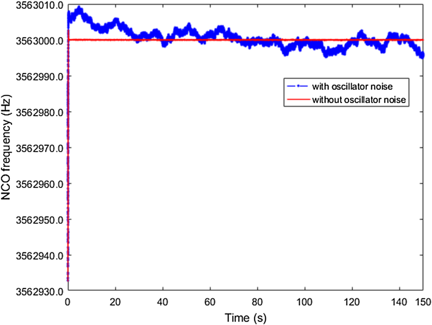
Figure 11. NCO frequency with and without oscillator noise.

Figure 12. Oscillator induced Doppler and ADR.
Typically, a Phase Lock Indicator (PLI) is used to assess the carrier phase tracking performance. Under strong signal conditions, PLI is approximately equal to cos(2δ ϕ), where δϕ is the phase difference between the local replica and the received signal (Bhaskar et al., Reference Bhaskar, Curran and Lachapelle2015). The PLI value approaches 1 when the phase tracking error is small enough, and −1 when the locally generated carrier is out of phase with the received signal. A value lower than 0·9 would not typically be used in carrier phase positioning applications (Aumayer and Petovello, Reference Aumayer and Petovello2016). Figure 13 shows the PLI value with and without oscillator noise considered, respectively. Since a lower loop bandwidth means more oscillator phase noise is not suppressed, the loop noise bandwidth is set to be 5 Hz in this work to enhance the oscillator phase noise effect. From Figure 13, we can see clearly that, when considering the oscillator phase noise, the PLI value decreases. It is worth noting that the PLI value is highly correlated with the oscillator frequency variations shown in Figure 11. Specifically, the PLI value drops greatly when the oscillator frequency variances exhibit steep slopes. This phenomenon is due to the oscillator dynamic effect on the phase tracking performance. As shown in Figure 13, the oscillator results in a radial velocity of about -4 m/s at around 25 s. This dynamic degrades the PLL tracking performance. This also verifies the necessity of considering oscillator effect when simulating IF signal sources for software receivers.

Figure 13. PLL lock detector.
5. CONCLUSION
This paper proposes a method to simulate the GNSS IF signal considering the oscillator phase noise. A pseudolite transmitter and receiver system is developed to accurately measure the oscillator parameters, with a percentage error of 2·22% for σy(0·001s), 2·11% for σy(0·01s), 0·93% for σy(0·1s), and 4·32% for σy(ls). The generated oscillator frequency fluctuations are shown to be well coincident with the oscillator under test, with percentage errors of 4·43%, 0·70%, 1·85% and 0·33% for ADEV values at averaging intervals of 0·001s, 0·01s, 0·1s and 1s, respectively. The oscillator phase noise effect on the tracking performance is also presented from the perspective of NCO frequency adjustment and the PLL lock detector, respectively. Results verify the effectiveness of this measuring system, and the necessity of oscillator phase noise when simulating the IF signal, in order to provide a software receiver with a better test environment.
This paper highlights the effect of simulated oscillator phase noise. Other factors (e.g., multipath interference) that also affect a receiver's performance will be considered to generate high-quality GNSS IF signals in future work.
ACKNOWLEDGMENTS
This work was supported by National Natural Science Foundation of China (grant number 60904085); Foundation of National Key Laboratory of Transient Physics; and Foundation of Defence Technology Innovation Special Filed.


