Nomenclature
Latin Symbols
- b
span
- c
local coefficient, chord length
- C
integral coefficient
-
 $c_{fx}$
x-component of skin friction coefficient
-
$\vec{C}_{WF}$
vector of force and moment coefficients of wing and fuselage
- d
diameter
-
$F_C$
centrifugal force
-
$F_D$
drag
-
$F_L$
lift
-
$F_M$
weight
-
$F_Q$
lateral force
-
$F_r$
radial force
-
$F_T$
thrust
-
$f_{t2}$
laminar suppression term in the SA turbulence model
- g
gravitational acceleration
- h
altitude
- m
mass
-
$M_B$
bending moment
-
$M_S$
swing moment
-
$M_T$
torsional moment
-
$M_x$
moment around x-axis
-
$M_y$
moment around y-axis
-
$M_{y0}$
zero-lift moment around y-axis
-
$M_{yCG}$
moment around y-axis evaluated at centre of gravity
-
$M_z$
moment around z-axis
- M
Mach number
-
$\mathit{M}_A$
manoeuvring Mach number
-
$\mathit{M}_C$
cruising Mach number
-
$\mathit{M}_D$
dive Mach number
-
$\mathit{M}_{MO}$
maximum operating Mach number
-
$\mathit{M}_{S1}$
stall Mach number
- MAC
mean aerodynamic chord
- MPL
maximum payload
- MTOW
maximum take-off weight
-
$n_z$
load factor
- p
pressure
- q
pitching rate, stagnation pressure
- R
design range, radius of circular flight path during pitching manoeuvre
- Re
Reynolds number
-
$res_\rho$
root mean square of density residual
- S
reference area
- V
airspeed
-
$x_{CG}$
position of centre of gravity
-
$x_{MAC25T-CG}$
distance between
$25\% \: MAC_T$
and centre of gravity-
$x_{MAC25T-MAC25W}$
distance between
$25\% \: MAC_T$
and
$25\% \: MAC_W$
-
$x_{MAC25W-CG}$
distance between
$25\% \: MAC_W$
and centre of gravity-
$x_N$
position of local neutral point
-
$y_{CGW}$
spanwise position of wing centre of gravity


Greek Symbols
-
$\alpha$
angle-of-attack
-
$\alpha_q$
additional angle-of-attack resulting from pitching motion
-
$\alpha_w$
downwash angle
-
$\beta$
damping coefficient
-
$\epsilon$
angle of incidence
-
$\eta$
dimensionless spanwise coordinate (
$\eta=0$
at wing root,
$\eta=1$
at wing tip), flap deflection-
$\lambda$
ratio of flap length to local chord
-
$\Lambda$
aspect ratio
-
$\nu$
dihedral
-
$\nu_e$
dihedral of elastic axis
-
$\xi$
aileron deflection, flap deflection
-
$\varphi$
sweep
-
$\varphi_{25}$
sweep of
$\frac{c}{4}$
-line-
$\varphi_e$
sweep of elastic axis
-
$\varphi_{LE}$
sweep of leading edge
-
$\omega$
grid rotation speed


Indices and Accents
- e
elevator
- f
flap
- F
fuselage
- i
iteration step
- T
tailplane
- tot
total
- W
wing
-
$\infty$
inflow

Abbreviations
- CFD
computational fluid dynamics
- DN
droop nose
- LA
load alleviation
- RANS
Reynolds-averaged Navier–Stokes
- SA
Spalart–Allmaras
- TEF
trailing-edge flap
1.0 Introduction
One key parameter that affects the efficiency of a transport aircraft is its weight. Commonly around 15–20% of the operational empty weight is allotted to the wing structure. The weight of the wing structure strongly depends on the loads the structure is designed for. The CS-25 [1], the EASA Certification Specifications and Acceptable Means of Compliance for Large Aeroplanes, define the load cases that need to be considered during design. In flight, those are several gust and manoeuvre load cases. To decrease those loads and thereby allow for the design of lighter structures, the concept of load alleviation can be applied.
The idea of alleviating loads originates from rotary wing technology. In 1912, Bartha et al. filed a patent [Reference Bartha and Madzsar2] that describes the concept of the flapping hinge. It serves different purposes, e.g. stabilising the rotor, but the main aspect according to Bartha et al. is the favourable effect of the strong reduction of bending moment at the blade root. Such a flapping hinge was first installed on an aircraft in 1923, when de la Cierva constructed his famous Autogiro [Reference Moreno-Caracciolo3] that was one of the first functioning rotary wing aircraft in aviation history.
Since the 1930s, load alleviation has also been a topic for research on fixed wing aircraft. The focus here was mainly on gust load alleviation that further offers the possibility to reduce accelerations under gusty conditions and thereby improve passenger comfort for civil applications or reliability for bombers. Many different concepts have been investigated [Reference McLean4] and more are under development [Reference Klug, Radespiel, Ullah, Seel, Lutz, Wild, Heinrich and Streit5, Reference Asaro, Khalil and Bauknecht6]. The most promising approach seems to be a load alleviation system that uses a combination of actuators at the leading and trailing edge of the wing. However, applying only gust load alleviation will not allow for a significant reduction of wing structure weight since constraints due to high manoeuvre loads still exist. So to exploit its full potential, gust load alleviation also requires a good concept for manoeuvre load alleviation.
Manoeuvre load alleviation can be achieved by changing the spanwise lift distribution. During a nose-up pitching manoeuvre, for example, the lift at the outboard wing is decreased and compensated by an increase of the lift at the inboard wing, resulting in a reduction of the bending moment along the whole span. As for gust load alleviation, this can be done by deflecting suitable control surfaces. Obviously it is now desirable to combine gust and manoeuvre load alleviation into one system using the same control surfaces. Compatibility was confirmed in the B-52 Control Configured Vehicles Program [Reference Hodges and McKenzie7] by flight testing a load alleviation system installed on a Boeing B-52E Stratofortress. These flight tests further demonstrated the possibility of integrating even more functionality such as active flutter control or improved flying qualities and stability. Several quasi-steady and unsteady manoeuvres were investigated, e.g. pitching manoeuvres, rolling manoeuvres and turns. The goal was a 10% reduction in wing-root bending moment, which could be achieved for every considered manoeuvre. Results showed that the most critical case is a quasi-steady nose-up pitching manoeuvre at maximum load factor and low speed. Higher speeds lead to elastic torsion that unloads the outer part of the swept-back wing.
An example of successful usage of manoeuvre load alleviation in operations is the Lockheed C-5A Galaxy. This aircraft was equipped with a gust and manoeuvre load alleviation system within the scope of the Active Lift Distribution Control System Program [Reference Disney8]. The system deflects ailerons and elevator as a function of inertial sensors, pitching rate and Mach number. The goal of a 30% reduction in incremental wing-root bending moment could be attained that way, but the negatively deflected ailerons for nose-up pitching manoeuvres led to an increase of incremental wing-root torsional moment of the same order of magnitude.
The problem of increasing torsional moments was also observed during design of the Lockheed L-1011-500, a long-range version of the Lockheed L-1011 TriStar. To increase range, the span of the aircraft was extended. This induces additional loads, so the outboard aileron was extended too. The outboard aileron was then used for manoeuvre load alleviation, similar to the Lockheed C-5A Galaxy discussed above. Ramsey et al. [Reference Ramsey and Lewolt9] examine the effect of increasing torsional moments on the basis of the wing structure design of the aircraft. They find that the effect on structural weight cannot be neglected, but all in all, the bending moment is of greater importance.
From the perspective of flight mechanics, the increase in wing torsional moment even provides some benefits. It reduces negative trim lift and thereby the required wing lift and wing bending moment. Further, trim drag is reduced, which can be beneficial for military applications [Reference Anderson, Berger and Hess10].
A comparison of manoeuvre load alleviation concepts for transport aircraft using different types and positions of control surfaces is provided by White [Reference White11]. Some of the investigated concepts are somewhat exotic and not very practical. On the other hand, White achieves good results for rather simple concepts using only ailerons and trailing-edge flaps. It could be shown, for example, that extending the span by 10% and using only ailerons for load alleviation allows for a
 $4.5 \text{t}$
increase in payload and an increase in range for a
$4.5 \text{t}$
increase in payload and an increase in range for a
 $318 \text{t}$
aircraft. In this context, White also points out some other, secondary effects related to load alleviation that must be considered too.
$318 \text{t}$
aircraft. In this context, White also points out some other, secondary effects related to load alleviation that must be considered too.
Within the scope of the research project PoLamin, several concepts for gust load alleviation using different control surfaces on wing and fuselage were investigated [Reference Klug, Radespiel, Ullah, Seel, Lutz, Wild, Heinrich and Streit5, Reference Klug, Naik, Ullah, Lutz, Wild, Heinrich and Radespiel12]. Amongst others, a load alleviation system for a generic swept-back transport aircraft, the so-called LEISA configuration [Reference Wild13], was derived. For this purpose, four separately controllable plain flaps were placed at the trailing edge of the single-slotted high-lift flap and a droop nose divided into five segments was placed at the leading edge [Reference Ullah, Lutz, Klug, Radespiel and Wild14].
The present study is part of the INTELWI project that began in 2020 as a collaborative research effort between TU Braunschweig, Universität Stuttgart, TU Hamburg, DLR, Airbus and others. One goal of this project is to design a manoeuvre load alleviation system based on dynamic control surface deflections for the LEISA aircraft. In the first step, the results from the PoLamin project are picked up and the designed load alleviation system is evaluated regarding its capability of alleviating manoeuvre loads. This requires the identification of critical manoeuvres as well as the development of methods to calculate those manoeuvres. Both aspects are the focus of the present study.
Relevant manoeuvres are chosen based on the CS-25 [1]. Pitching manoeuvres with different load factors at different Mach numbers and altitudes are considered. Manoeuvre loads are calculated with a new method based on a combination of handbook formulas and computational fluid dynamics (CFD). While the parameters of manoeuvre flight are estimated via handbook formulas, the actual manoeuvre is calculated with three-dimensional RANS simulations of the aircraft without empennage. The manoeuvres are computed as quasi-steady state; unsteady effects during the initiation of a manoeuvre are neglected. Further, the aircraft is considered as a rigid body, so static and dynamic aeroelastic effects are neglected, too.
The present study chooses a single manoeuvre for simulating load alleviation. Comparison with the manoeuvre without load alleviation then demonstrates the potential of the considered load alleviation system. Moreover, the physics and the secondary effects coming along with load alleviation are analysed. Finally, a suggestion is made on how to further improve calculation methods and load alleviation technology on the basis of the present results.
2.0 Problem description
2.1 The LEISA aircraft
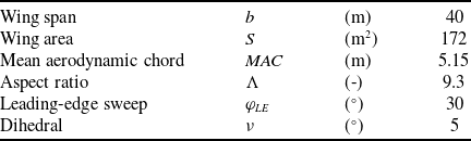
The LEISA configuration is a generic swept-back transport aircraft configuration that was designed at DLR Braunschweig [Reference Wild13] and has been used as a reference aircraft in various research projects [Reference Pott-Pollenske, Wild and Bertsch15]. Figure 1 shows sketches of the aircraft from three perspectives. Essential data regarding size, range and wing geometry are presented in Tables 1 and 2. With a maximum take-off weight of
 $85,290\text{kg}$
and a maximum payload of
$85,290\text{kg}$
and a maximum payload of
 $25,000\text{kg}$
, the LEISA configuration is slightly larger than the Airbus A320-200.
$25,000\text{kg}$
, the LEISA configuration is slightly larger than the Airbus A320-200.
Table 1. Weights and range of the LEISA configuration [Reference Wild13]
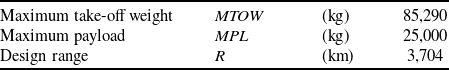
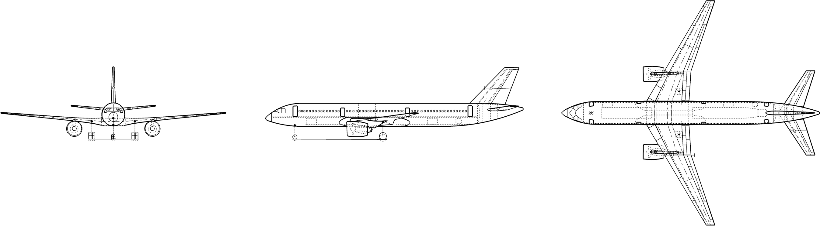
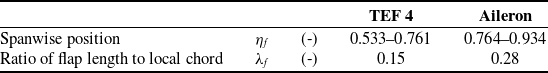
Table 2. Geometrical parameters of the LEISA wing [Reference Wild13]


Figure 1. Three-view drawing of the LEISA configuration [Reference Heinze, Haupt and Woidt16].
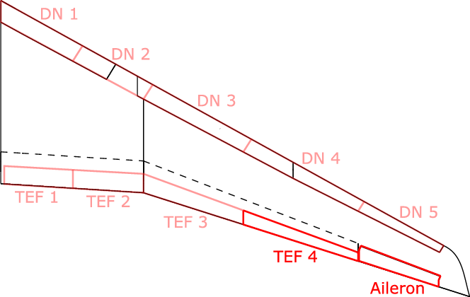
Figure 2 shows the geometry of the wing, including the relevant control surfaces. The high-lift system originally consists of a leading-edge slat over the whole span with a cut-out at the engine position and a single-slotted flap at the trailing edge from the wing root to the aileron [Reference Wild13]. Here, the slat is replaced by a droop nose (DN) divided into five segments; at the trailing edge of the high-lift flap, four separately controllable plain flaps (TEF) are placed. Combined with the aileron, these movables can be used for load alleviation [Reference Ullah, Lutz, Klug, Radespiel and Wild14]. However, within the scope of this study, only the outermost trailing-edge flap and the aileron are considered. This simplifies the present task to evaluate the potential for load alleviation. Similar concepts performed well as discussed by Disney [Reference Disney8], Ramsey et al. [Reference Ramsey and Lewolt9] and White [Reference White11]. The geometrical parameters of the used control surfaces are presented in Table 3.
2.2 Considered manoeuvres
The selection of the considered manoeuvres is based on the CS-25 [1]. According to these requirements, quasi-steady as well as unsteady manoeuvres need to be taken into account for the certification of an aircraft. In this study, only quasi-steady manoeuvres are discussed since Hodges et al. [Reference Hodges and McKenzie7] and Ramsey et al. [Reference Ramsey and Lewolt9] show that loads resulting from this kind of manoeuvre are critical for most parts of the wing structure.
For symmetrical manoeuvres, the evaluation of certification specifications for the LEISA configuration yields the manoeuvring envelope sketched in Fig. 3. Regions with deployed high-lift system at low speeds are neglected here. The manoeuvring envelope is a function of altitude.
 $\mathrm{M}_{S1}$
denotes the stall Mach number, the lowest Mach number at which steady flight with a load factor of
$\mathrm{M}_{S1}$
denotes the stall Mach number, the lowest Mach number at which steady flight with a load factor of
 $n_z=1$
is possible.
$n_z=1$
is possible.
 $\mathrm{M}_{S1}$
increases with increasing altitude because of decreasing stagnation pressure, and so does the manoeuvring Mach number
$\mathrm{M}_{S1}$
increases with increasing altitude because of decreasing stagnation pressure, and so does the manoeuvring Mach number
 $\mathrm{M}_A$
, the lowest Mach number where the maximum load factor of
$\mathrm{M}_A$
, the lowest Mach number where the maximum load factor of
 $n_z=2.5$
can be reached. The cruising Mach number
$n_z=2.5$
can be reached. The cruising Mach number
 $\mathrm{M}_C$
(
$\mathrm{M}_C$
(
 $0.80$
), maximum operating Mach number
$0.80$
), maximum operating Mach number
 $\mathrm{M}_{MO}$
(
$\mathrm{M}_{MO}$
(
 $0.85$
) and dive Mach number
$0.85$
) and dive Mach number
 $\mathrm{M}_D$
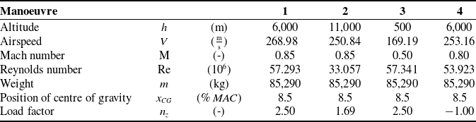
are independent of altitude. Based on this envelope, four pitching manoeuvres at different Mach numbers and altitudes are chosen, as also displayed in Fig. 3. Additional parameters of manoeuvre flight are presented in Table 4.
$\mathrm{M}_D$
are independent of altitude. Based on this envelope, four pitching manoeuvres at different Mach numbers and altitudes are chosen, as also displayed in Fig. 3. Additional parameters of manoeuvre flight are presented in Table 4.
Table 3. Geometrical parameters of the control surfaces used for load alleviation


Figure 2. Slightly distorted view of the LEISA wing including the control surfaces of the load alleviation system.
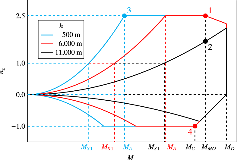
Figure 3. Manoeuvring envelope at different altitudes and considered pitching manoeuvres.
Table 4. Overview of considered manoeuvres

Manoeuvre 1 is a nose-up pitching manoeuvre at medium altitude
 $h=6,000\text{m}$
, maximum load factor
$h=6,000\text{m}$
, maximum load factor
 $n_z=2.5$
and maximum operating Mach number
$n_z=2.5$
and maximum operating Mach number
 $\mathrm{M}_{MO}=0.85$
.
$\mathrm{M}_{MO}=0.85$
.
Manoeuvre 2 describes a nose-up pitching manoeuvre at typical cruising altitude
 $h=11,000\text{m}$
, also at
$h=11,000\text{m}$
, also at
 $\mathrm{M}_{MO}=0.85$
. The maximum achievable load factor at this altitude is
$\mathrm{M}_{MO}=0.85$
. The maximum achievable load factor at this altitude is
 $n_z=1.69$
.
$n_z=1.69$
.
For manoeuvre 3, which is also a nose-up pitching manoeuvre, the manoeuvring Mach number
 $\mathrm{M}_A$
and maximum load factor
$\mathrm{M}_A$
and maximum load factor
 $n_z=2.5$
are chosen. Since also a low Mach number should be investigated, a low altitude of
$n_z=2.5$
are chosen. Since also a low Mach number should be investigated, a low altitude of
 $h=500\text{m}$
is chosen here. The manoeuvring Mach number at this altitude was initially estimated as
$h=500\text{m}$
is chosen here. The manoeuvring Mach number at this altitude was initially estimated as
 $\mathrm{M}_A=0.50$
, slightly above the true value of
$\mathrm{M}_A=0.50$
, slightly above the true value of
 $\mathrm{M}_A=0.48$
.
$\mathrm{M}_A=0.48$
.
Manoeuvre 4 is a nose-down pitching manoeuvre at cruising Mach number
 $\mathrm{M}_C=0.80$
. Since the desired load factor
$\mathrm{M}_C=0.80$
. Since the desired load factor
 $n_z=-1$
cannot be achieved at cruising altitude, a lower altitude of
$n_z=-1$
cannot be achieved at cruising altitude, a lower altitude of
 $h=6,000\text{m}$
is chosen.
$h=6,000\text{m}$
is chosen.
For all manoeuvres, the centre of gravity is assumed to be at a forward position at
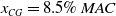 $x_{CG}=8.5\% \: MAC$
. In this case, e.g. during a nose-up pitching manoeuvre, the tailplane generates high negative lift and the wing yields high positive lift, resulting in high manoeuvre loads. A critical loading condition should be considered, so the maximum aircraft weight of
$x_{CG}=8.5\% \: MAC$
. In this case, e.g. during a nose-up pitching manoeuvre, the tailplane generates high negative lift and the wing yields high positive lift, resulting in high manoeuvre loads. A critical loading condition should be considered, so the maximum aircraft weight of
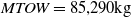 $MTOW=85,\!290\text{kg}$
is chosen for all four manoeuvres. Technically, the case with maximum payload, maximum fuel inside the fuselage and the inboard wing tanks, but with empty outboard wing tanks would be even more critical in terms of loads. Because the centre of gravity of the outboard wing tanks is located further outboard than the centre of lift distribution, the decreasing effect on wing bending moment resulting from inertia forces on the fuel inside the tanks is stronger than the increasing effect on wing bending moment resulting from the additional lift required. However, as part of the load alleviation concept, it is assumed that those fuelling conditions are avoided, making the case with maximum total weight critical.
$MTOW=85,\!290\text{kg}$
is chosen for all four manoeuvres. Technically, the case with maximum payload, maximum fuel inside the fuselage and the inboard wing tanks, but with empty outboard wing tanks would be even more critical in terms of loads. Because the centre of gravity of the outboard wing tanks is located further outboard than the centre of lift distribution, the decreasing effect on wing bending moment resulting from inertia forces on the fuel inside the tanks is stronger than the increasing effect on wing bending moment resulting from the additional lift required. However, as part of the load alleviation concept, it is assumed that those fuelling conditions are avoided, making the case with maximum total weight critical.
Other parameters needed for the simulation of the respective manoeuvres, e.g. control surface deflections, angle-of-attack or pitching rate, are determined on the basis of the methods discussed in the following Section 3.
3.0 Calculation methods
3.1 Approach
The manoeuvres described in Section 2.2 are calculated on the basis of CFD simulations and handbook formulas. For better efficiency, only the wing and fuselage of the LEISA aircraft are considered in the CFD simulations, whereas the effect of the tailplane is considered via handbook methods. For a pitching manoeuvre, the contribution of the tailplane to the lift and pitching moment has to be known to determine the angle-of-attack at which a certain load factor is achieved. Thus, handbook methods serve the purpose of providing the manoeuvre flight parameters needed for the actual CFD simulations. Furthermore, on the basis of handbook calculations and some CFD simulations serving as nodes, the wing loading within the whole flight envelope is interpolated or extrapolated. This approach has the advantage that it combines high precision for the simulation of specific manoeuvres provided by Navier–Stokes methods and the high efficiency for calculations within the whole flight envelope as an advantage of handbook methods. The method was developed within the scope of this study and, to the authors’ best knowledge, has not been applied anywhere else yet.
3.2 Manoeuvre calculation
The pitching manoeuvre is treated as quasi-steady, meaning unsteady processes during the initiation of the manoeuvre are neglected. The angle-of-attack and pitching rate are therefore considered as constant during the manoeuvre, and all forces and moments acting on the aircraft are balanced. This equilibrium of forces and moments is the basis for the calculation methods presented in the following.
The forces and moments acting on the aircraft are sketched in Fig. 4. Note that forces in circumferential direction of aircraft motion are not further considered. Also the contribution of thrust
 $F_T$
in the radial direction is neglected. Balancing the forces in the radial direction and the pitching moments around the centre of gravity yields
$F_T$
in the radial direction is neglected. Balancing the forces in the radial direction and the pitching moments around the centre of gravity yields
 \begin{eqnarray} \sum F_{r,tot} = &F_C + F_M - ( F_{LW} + F_ {LF} ) - F_{LT} = 0 \ ,\end{eqnarray}
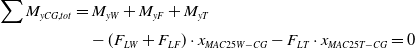 \begin{align} \sum M_{yCG,tot} &= M_{yW} + M_{yF} + M_{yT} \nonumber\\ & \quad - (F_{LW} + F_{LF}) \cdot x_{MAC25W-CG} - F_{LT} \cdot x_{MAC25T-CG} = 0\end{align}
where the moments acting on wing and fuselage are evaluated at 25% of mean aerodynamic chord of the wing and the moment acting on the tailplane is evaluated at 25% of mean aerodynamic chord of the tailplane. Hence,
 $x_{MAC25-CG}$
is the lever arm of respective forces at the centre of gravity.
$x_{MAC25-CG}$
is the lever arm of respective forces at the centre of gravity.
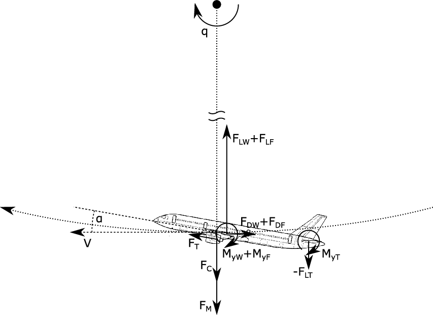
Figure 4. Forces and moments acting on the aircraft during the pitching manoeuvre.
Evaluation of the weight
 $F_M=mg$
and centrifugal force
$F_M=mg$
and centrifugal force
 $F_C=mVq$
is trivial. From the definition of the load factor
$F_C=mVq$
is trivial. From the definition of the load factor
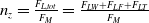 $n_z=\frac{F_{L,tot}}{F_M}=\frac{F_{LW}+F_{LF}+F_{LT}}{F_M}$
, one obtains
$n_z=\frac{F_{L,tot}}{F_M}=\frac{F_{LW}+F_{LF}+F_{LT}}{F_M}$
, one obtains
 \begin{eqnarray} q = (n_z - 1) \frac{g}{V}\end{eqnarray}
for the pitching rate.
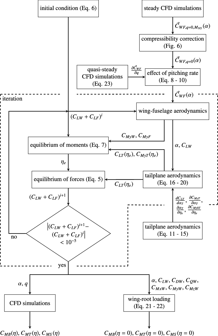
A pitching manoeuvre requires a certain angle-of-attack dependent on the desired load factor, Mach number and altitude. The angle-of-attack is calculated iteratively by means of the method illustrated in Fig. 5. In the following, this approach is described in more detail.

Figure 5. Iterative calculation of the pitching manoeuvre based on a combination of handbook and Navier–Stokes methods; blocks and arrows inside the dashed box are part of the actual iteration; other blocks have to be evaluated only once for each manoeuvre.
Firstly, the equilibrium of forces from Equation (1) is written in coefficient form as
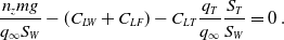 \begin{eqnarray} \frac{n_z mg}{q_\infty S_W} - ( C_{LW} + C_{LF} ) - C_{LT} \frac{q_T}{q_\infty} \frac{S_T}{S_W} = 0 \ .\end{eqnarray}
It is assumed that
 $\frac{q_T}{q_\infty}=0.99$
. This factor takes into account that the tailplane is located in the wake of the wing and is therefore exposed to a lower stagnation pressure. From Equation (4), the iteration rule for the lift coefficient of wing and fuselage is derived as
$\frac{q_T}{q_\infty}=0.99$
. This factor takes into account that the tailplane is located in the wake of the wing and is therefore exposed to a lower stagnation pressure. From Equation (4), the iteration rule for the lift coefficient of wing and fuselage is derived as
 \begin{eqnarray} (C_{LW} + C_{LF})^{i+1} = (C_{LW} + C_{LF})^i + \beta \cdot \left( \frac{n_z mg}{q_\infty S_W} - (C_{LW} + C_{LF})^i - C_{LT}^i \frac{q_T}{q_\infty} \frac{S_T}{S_W} \right) \ .\end{eqnarray}
This corresponds to the damped Newton’s method with
 $\beta=0.1$
as damping coefficient.
$\beta=0.1$
as damping coefficient.
As the initial condition for the iteration,
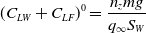 \begin{eqnarray} (C_{LW} + C_{LF})^0 = \frac{n_z mg}{q_\infty S_W}\end{eqnarray}
is chosen. To evaluate Equation (5), the lift coefficient of the tailplane
 $C_{LT}$
first needs to be determined. Considering the equilibrium of moments from Equation (2) written in coefficient form as
$C_{LT}$
first needs to be determined. Considering the equilibrium of moments from Equation (2) written in coefficient form as
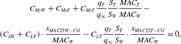 \begin{eqnarray} &C_{MyW} + C_{MyF} + C_{MyT} \dfrac{q_T}{q_\infty} \dfrac{S_T}{S_W} \dfrac{MAC_T}{MAC_W} - \nonumber\\[5pt] &(C_{LW} + C_{LF}) \cdot \dfrac{x_{MAC25W-CG}}{MAC_W} - C_{LT} \dfrac{q_T}{q_\infty} \dfrac{S_T}{S_W} \cdot \dfrac{x_{MAC25T-CG}}{MAC_W} = 0,\end{eqnarray}
where the moments acting on the wing and fuselage are normalised using the mean aerodynamic chord of the wing and the moment acting on the tailplane is normalised using the mean aerodynamic chord of the tailplane, the remaining unknowns are
 $C_{MyW}$
,
$C_{MyW}$
,
 $C_{MyF}$
,
$C_{MyF}$
,
 $C_{LT}$
and
$C_{LT}$
and
 $C_{MyT}$
. For the present study, the geometrical parameters of the tailplane are provided by Wild [Reference Wild17].
$C_{MyT}$
. For the present study, the geometrical parameters of the tailplane are provided by Wild [Reference Wild17].
At this point
 $C_{MyW}$
,
$C_{MyW}$
,
 $C_{MyF}$
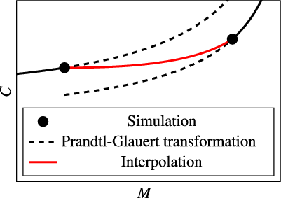
, the respective angle-of-attack and all other forces and moments acting on the wing–fuselage configuration are determined by the use of Navier–Stokes methods. For this purpose, CFD simulations at certain Mach numbers and different angles of attack were carried out as described in Section 3.3. Since CFD results are available for specific Mach numbers only, the effect of compressibility needs to be corrected to obtain also values at other Mach numbers. Effects on the aerodynamics of the fuselage are neglected; only the forces and moments acting on the wing are adjusted. For this, the Prandtl–Glauert transformation as described by Schlichting et al. [Reference Schlichting and Truckenbrodt18] (pp 171–173) is used. Strictly speaking, this transformation applies to two-dimensional flow only, but according to Göthert [Reference Göthert19], it is a good approximation for wings with high aspect ratio, too. After correcting the simulation results at the next highest Mach number and those at the next lowest Mach number, linear interpolation regarding the Mach number of the particular manoeuvre is performed between both cases, as illustrated in Fig. 6. That way, information from simulations at different Mach numbers is considered as well as nonlinear effects of compressibility. If the Mach number lies outside of the range covered by simulations, the Prandtl–Glauert-corrected results from the simulations at the nearest Mach number are applied directly.
$C_{MyF}$
, the respective angle-of-attack and all other forces and moments acting on the wing–fuselage configuration are determined by the use of Navier–Stokes methods. For this purpose, CFD simulations at certain Mach numbers and different angles of attack were carried out as described in Section 3.3. Since CFD results are available for specific Mach numbers only, the effect of compressibility needs to be corrected to obtain also values at other Mach numbers. Effects on the aerodynamics of the fuselage are neglected; only the forces and moments acting on the wing are adjusted. For this, the Prandtl–Glauert transformation as described by Schlichting et al. [Reference Schlichting and Truckenbrodt18] (pp 171–173) is used. Strictly speaking, this transformation applies to two-dimensional flow only, but according to Göthert [Reference Göthert19], it is a good approximation for wings with high aspect ratio, too. After correcting the simulation results at the next highest Mach number and those at the next lowest Mach number, linear interpolation regarding the Mach number of the particular manoeuvre is performed between both cases, as illustrated in Fig. 6. That way, information from simulations at different Mach numbers is considered as well as nonlinear effects of compressibility. If the Mach number lies outside of the range covered by simulations, the Prandtl–Glauert-corrected results from the simulations at the nearest Mach number are applied directly.

Figure 6. Determination of the aerodynamic coefficients as a function of Mach number.
Besides the steady aerodynamics of the wing–fuselage configuration, the effect of pitching rate is examined. Accordingly, the forces and moments from the steady CFD simulations are adjusted on the basis of quasi-steady simulations that are also described in Section 3.3. With
 \begin{eqnarray} \vec{C}_{WF} = (C_{LW}, \: C_{DW}, \: C_{QW}, \: C_{MxW}, \: C_{MyW}, \: C_{MzW}, \: C_{LF}, \: C_{DF}, \: C_{QF}, \: C_{MxF}, \: C_{MyF}, \: C_{MzF})^T\end{eqnarray}
as a vector of the force and moment coefficients of wing and fuselage, one obtains
 \begin{eqnarray} \vec{C}_{WF} (\alpha) = \vec{C}_{WF,q=0} (\alpha) + \frac{\partial \vec{C}_{WF}}{\partial q} q \ .\end{eqnarray}
 $\frac{\partial \vec{C}_{WF}}{\partial q}$
must be determined in preliminary quasi-steady CFD simulations. However, for most parts of this study, the effect of pitching rate on the aerodynamics of wing and fuselage is neglected. In those cases, this step can be omitted, leading to
$\frac{\partial \vec{C}_{WF}}{\partial q}$
must be determined in preliminary quasi-steady CFD simulations. However, for most parts of this study, the effect of pitching rate on the aerodynamics of wing and fuselage is neglected. In those cases, this step can be omitted, leading to
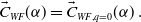 \begin{eqnarray} \vec{C}_{WF} (\alpha) = \vec{C}_{WF,q=0} (\alpha) \ .\end{eqnarray}
Now that the results from CFD simulations are prepared, the angle-of-attack required for a specific manoeuvre as well as all integral forces and moments acting on the aircraft during this manoeuvre can be linearly interpolated regarding the lift coefficients of wing and fuselage. Thus,
 $C_{MyW}$
and
$C_{MyW}$
and
 $C_{MyF}$
are now known and can be inserted into the equilibrium of moments in Equation (7).
$C_{MyF}$
are now known and can be inserted into the equilibrium of moments in Equation (7).
To find the relation between the two remaining unknowns
 $C_{LT}$
and
$C_{LT}$
and
 $C_{MyT}$
, the aerodynamics of the tailplane are examined. From formulas stated by Schlichting et al. [Reference Schlichting and Truckenbrodt18] (pp. 70, 405), the slope of the lift curve of the tailplane can be derived as
$C_{MyT}$
, the aerodynamics of the tailplane are examined. From formulas stated by Schlichting et al. [Reference Schlichting and Truckenbrodt18] (pp. 70, 405), the slope of the lift curve of the tailplane can be derived as
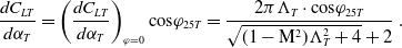 \begin{eqnarray} \frac{d C_{LT}}{d \alpha_T} = \left( \frac{d C_{LT}}{d \alpha_T} \right)_{\varphi = 0} \text{cos} \varphi_{25T} = \frac{2 \pi \Lambda_T \cdot \text{cos} \varphi_{25T}}{\sqrt{(1-\mathrm{M}^2) \Lambda_T^2 + 4}+2} \ .\end{eqnarray}
For simplification, it is assumed that the tailplane aerofoil is symmetrical so that the lift force acts approximately on its
 $\frac{c}{4}$
-point. Hence,
$\frac{c}{4}$
-point. Hence,
 \begin{eqnarray} \frac{\partial C_{MyT}}{\partial \alpha_T} = 0\end{eqnarray}
follows for the slope of the moment around the
 $\frac{c}{4}$
-point and
$\frac{c}{4}$
-point and
 \begin{eqnarray} C_{My0T, \eta_e = 0} = 0\end{eqnarray}
follows for the zero-lift moment coefficient without elevator deflection
 $\eta_e$
.
$\eta_e$
.
Besides the angle-of-attack, also the deflection of the elevator contributes to the equilibrium of forces and moments. According to Schlichting et al. [Reference Schlichting and Truckenbrodt18] (pp. 440, 446), the respective lift coefficient can be considered by adjusting the angle-of-attack:
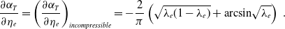 \begin{eqnarray} \frac{\partial \alpha_T}{\partial \eta_e} = \left( \frac{\partial \alpha_T}{\partial \eta_e} \right)_{incompressible} = - \frac{2}{\pi} \left( \sqrt{\lambda_e ( 1 - \lambda_e ) } + \text{arcsin} \sqrt{\lambda_e} \right) \ .\end{eqnarray}
The change in zero-lift moment coefficient is calculated, also according to Schlichting et al. [Reference Schlichting and Truckenbrodt18] (p. 446) [Reference Schlichting and Truckenbrodt20] (p. 430), via
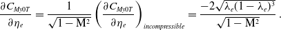 \begin{eqnarray} \frac{\partial C_{My0T}}{\partial \eta_e} = \frac{1}{\sqrt{1-\mathrm{M}^2}} \left( \frac{\partial C_{My0T}}{\partial \eta_e} \right)_{incompressible} = \frac{-2 \sqrt{\lambda_e ( 1 - \lambda_e )^3}}{\sqrt{1-\mathrm{M}^2}} \ .\end{eqnarray}
The angle-of-attack at the tailplane results from superposition:
 \begin{eqnarray} \alpha_T = \alpha + \epsilon_T + \alpha_w + \alpha_q \ .\end{eqnarray}
Here,
 $\epsilon_T$
is the angle of incidence of the tailplane. By adding
$\epsilon_T$
is the angle of incidence of the tailplane. By adding
 $\alpha_w$
, the downwash induced by the wing is taken into account. It can be calculated via
$\alpha_w$
, the downwash induced by the wing is taken into account. It can be calculated via
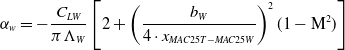 \begin{eqnarray} \alpha_w = - \frac{C_{LW}}{\pi \Lambda_W} \left[ 2+ \left( \frac{b_W}{4 \cdot x_{MAC25T-MAC25W}} \right)^2 (1-\mathrm{M}^2) \right]\end{eqnarray}
where
 $x_{MAC25T-MAC25W}$
denotes the distance between the wing and tailplane [Reference Schlichting and Truckenbrodt18] (p 407).
$x_{MAC25T-MAC25W}$
denotes the distance between the wing and tailplane [Reference Schlichting and Truckenbrodt18] (p 407).
 $\alpha_q$
is an additional angle-of-attack that results from the pitching motion of the aircraft. As shown in Fig. 4, the aircraft is suspended at its centre of gravity. Due to the rotation, the tailplane is moved downwards with a velocity of
$\alpha_q$
is an additional angle-of-attack that results from the pitching motion of the aircraft. As shown in Fig. 4, the aircraft is suspended at its centre of gravity. Due to the rotation, the tailplane is moved downwards with a velocity of
 $q \cdot x_{MAC25T-CG}$
. This is equivalent to an additional angle-of-attack
$q \cdot x_{MAC25T-CG}$
. This is equivalent to an additional angle-of-attack
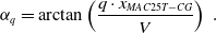 \begin{eqnarray} \alpha_q = \text{arctan} \left( \frac{q \cdot x_{MAC25T-CG}}{V} \right) \ .\end{eqnarray}
Finally, the lift coefficient of the tailplane
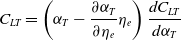 \begin{eqnarray} C_{LT} = \left( \alpha_T - \frac{\partial \alpha_T}{\partial \eta_e} \eta_e \right) \frac{d C_{LT}}{d \alpha_T}\end{eqnarray}
and its moment coefficient
 \begin{eqnarray} C_{MyT} = C_{My0T, \eta_e = 0} + \frac{\partial C_{My0T}}{\partial \eta_e} \eta_e + \frac{\partial C_{MyT}}{\partial \alpha_T} \left( \alpha_T - \frac{\partial \alpha_T}{\partial \eta_e} \eta_e \right) = \frac{\partial C_{My0T}}{\partial \eta_e} \eta_e\end{eqnarray}
can be evaluated. Equations (19) and (20) are inserted into the equilibrium of moments in Equation (7). Two unknowns remain: the angle of incidence
 $\epsilon_T$
and the elevator deflection
$\epsilon_T$
and the elevator deflection
 $\eta_e$
.
$\eta_e$
.
 $\epsilon_T$
is determined before the actual manoeuvre is calculated. For this purpose, the calculation method described in this section is applied to steady flight with
$\epsilon_T$
is determined before the actual manoeuvre is calculated. For this purpose, the calculation method described in this section is applied to steady flight with
 $n_z=1$
under the constraint
$n_z=1$
under the constraint
 $\eta_e=0$
. Thus, the aircraft is trimmed for level flight under the respective conditions, and the manoeuvre is then initiated by deflecting the elevator.
$\eta_e=0$
. Thus, the aircraft is trimmed for level flight under the respective conditions, and the manoeuvre is then initiated by deflecting the elevator.
At this point, the last remaining unknown
 $\eta_e$
can be determined by solving Equation (7). Thereby, the lift coefficient of the tailplane
$\eta_e$
can be determined by solving Equation (7). Thereby, the lift coefficient of the tailplane
 $C_{LT}$
is known and can be inserted into the iteration rule in Equation (5). The iteration is then repeated until the lift coefficient of the wing–fuselage configuration changes by less than
$C_{LT}$
is known and can be inserted into the iteration rule in Equation (5). The iteration is then repeated until the lift coefficient of the wing–fuselage configuration changes by less than
 $10^{-5}$
.
$10^{-5}$
.
Besides the angle-of-attack and the pitching rate that are used for further, more precise calculations based on Navier–Stokes methods, the combination of handbook methods and CFD simulations described in this section also yields the integral force and moment coefficients of the wing. These can be used for estimating the wing-root loading already at this point, allowing for an efficient calculation of manoeuvre loads within the whole flight envelope.
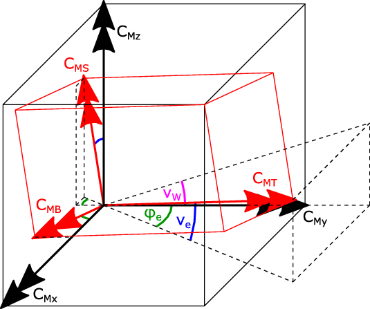
Because the moments in the global coordinate system of the aircraft are not very meaningful regarding design of the wing structure, they are transformed into the coordinate system of the wing as illustrated in Fig. 7. From this sketch, the respective transformation can be derived as
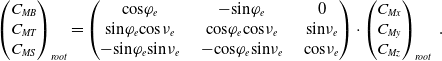 \begin{eqnarray} \begin{pmatrix} C_{MB} \\ C_{MT} \\ C_{MS} \end{pmatrix}_{root} = \begin{pmatrix} \text{cos} \varphi_e\;\;\;\;\; & -\text{sin} \varphi_e\;\;\;\;\; & 0 \\ \text{sin} \varphi_e \text{cos} \nu_e \;\;\;\;\; & \text{cos} \varphi_e \text{cos} \nu_e \;\;\;\;\; & \text{sin} \nu_e \\ -\text{sin} \varphi_e \text{sin} \nu_e \;\;\;\;\; & -\text{cos} \varphi_e \text{sin} \nu_e \;\;\;\;\; & \text{cos} \nu_e \end{pmatrix} \cdot \begin{pmatrix} C_{Mx} \\ C_{My} \\ C_{Mz} \end{pmatrix}_{root} \ .\end{eqnarray}
Here,
 $\varphi_e$
denotes the wing sweep at the elastic axis and
$\varphi_e$
denotes the wing sweep at the elastic axis and
 $\nu_e$
is the dihedral at the elastic axis. For simplification, it is assumed that the elastic axis is described by the straight connection line between the point at 45% chord at the wing root and the point at 45% chord at the wing tip.
$\nu_e$
is the dihedral at the elastic axis. For simplification, it is assumed that the elastic axis is described by the straight connection line between the point at 45% chord at the wing root and the point at 45% chord at the wing tip.

Figure 7. Wing-root moments in the global coordinate system of the aircraft and in the coordinate system of the wing.
Additional to the aerodynamic forces, engine thrust and inertial forces contribute to the wing loading. Engine thrust is neglected here, and the effect of inertial forces on torsional and swing moment is not considered either. However, inertial forces have a strong load alleviating effect on the wing bending moment. This can be taken into account by evaluating the expression
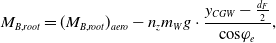 \begin{eqnarray} M_{B,root} = (M_{B,root})_{aero} - n_z m_W g \cdot \frac{y_{CGW}-\frac{d_F}{2}}{\text{cos} \varphi_e},\end{eqnarray}
where
 $m_W$
is the weight of the wing including engine and fuel,
$m_W$
is the weight of the wing including engine and fuel,
 $y_{CGW}$
is the spanwise position of its centre of gravity and
$y_{CGW}$
is the spanwise position of its centre of gravity and
 $d_F$
denotes the diameter of the fuselage. For the present study,
$d_F$
denotes the diameter of the fuselage. For the present study,
 $m_W$
and
$m_W$
and
 $y_{CGW}$
are taken from the structural model that was designed by Heinze et al. [Reference Heinze, Haupt and Woidt16] for an aircraft very similar to the LEISA aircraft.
$y_{CGW}$
are taken from the structural model that was designed by Heinze et al. [Reference Heinze, Haupt and Woidt16] for an aircraft very similar to the LEISA aircraft.
3.3 CFD simulation
Steady simulation
To determine the aerodynamics of the wing–fuselage configuration for the relevant Mach numbers, steady simulations at different angles of attack are carried out. A total of 20 cases (not including the cases beyond
 $C_{Lmax}$
that were disregarded) were used to create a database that is accessed during the calculations discussed in the previous Section 3.2. Amongst others, those calculations yield the angle-of-attack required for a specific manoeuvre. Neglecting the effect of pitching motion on wing–fuselage aerodynamics, steady simulations of the manoeuvres described in Section 2.2 can then be performed. Note that these results also include the spanwise distribution of manoeuvre loads.
$C_{Lmax}$
that were disregarded) were used to create a database that is accessed during the calculations discussed in the previous Section 3.2. Amongst others, those calculations yield the angle-of-attack required for a specific manoeuvre. Neglecting the effect of pitching motion on wing–fuselage aerodynamics, steady simulations of the manoeuvres described in Section 2.2 can then be performed. Note that these results also include the spanwise distribution of manoeuvre loads.
For the simulations, the DLR TAU-Code is used. The DLR TAU-Code solves the Navier–Stokes equations on hybrid unstructured grids using a finite volume method as described by Schwamborn et al. [Reference Schwamborn, Gerhold and Heinrich21] and Heinrich et al. [Reference Heinrich, Dwight, Widhalm and Raichle22]. Assuming symmetrical flow, three-dimensional RANS simulations of an idealised half model of the rigid LEISA configuration without engines and without empennage are carried out. For turbulence modelling, the SAO version of the one-equation SA model from Spalart and Allmaras is applied. In this implementation, the so-called
 $f_{t2}$
laminar suppression term is eliminated from the standard model, which is a reasonable approach for fully turbulent flows as stated by Allmaras et al. [Reference Allmaras, Johnson and Spalart23]. For the discretisation of convective fluxes, the second-order central scheme is used, while the chosen dissipation scheme relies on scalar dissipation. The simulation domain including boundary conditions and the respective grid is shown in Fig. 8(a) and (b), while the surface grid on the wing and fuselage is illustrated in (c). It features some refinement in the region of the wing where the shock is expected. Figure 8(d) contains the boundary-layer grid at the wing section
$f_{t2}$
laminar suppression term is eliminated from the standard model, which is a reasonable approach for fully turbulent flows as stated by Allmaras et al. [Reference Allmaras, Johnson and Spalart23]. For the discretisation of convective fluxes, the second-order central scheme is used, while the chosen dissipation scheme relies on scalar dissipation. The simulation domain including boundary conditions and the respective grid is shown in Fig. 8(a) and (b), while the surface grid on the wing and fuselage is illustrated in (c). It features some refinement in the region of the wing where the shock is expected. Figure 8(d) contains the boundary-layer grid at the wing section
 $\eta = 0.647$
for the case with load alleviation, thus with the trailing-edge flap deflected by
$\eta = 0.647$
for the case with load alleviation, thus with the trailing-edge flap deflected by
 $\xi = -15^\circ$
. The boundary layer grid consists of 50 cells in normal direction; the height of the first cell is on the order of
$\xi = -15^\circ$
. The boundary layer grid consists of 50 cells in normal direction; the height of the first cell is on the order of
 $y^+ \approx 1$
, as exemplarily shown for the simulation of manoeuvre 1 in Fig. 9(a).
$y^+ \approx 1$
, as exemplarily shown for the simulation of manoeuvre 1 in Fig. 9(a).
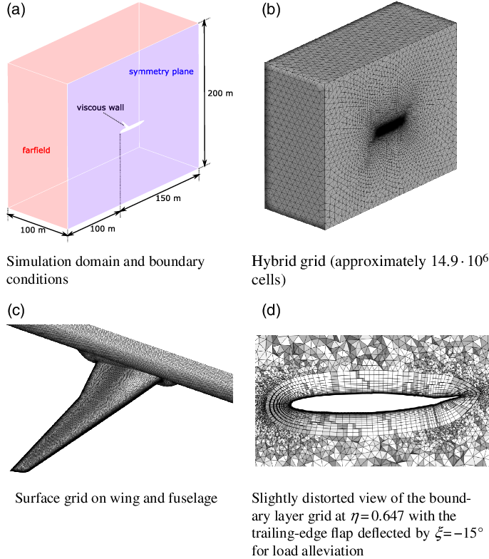
Figure 8. Domain and grid used for CFD simulations.
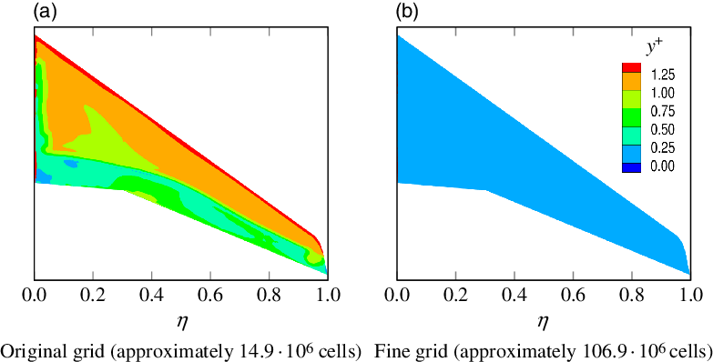
Figure 9. Distribution of
 $y^+$
on the upper surface of the wing for manoeuvre 1 from simulations on the original grid and on the fine grid.
$y^+$
on the upper surface of the wing for manoeuvre 1 from simulations on the original grid and on the fine grid.
One simulation usually takes about
 $2.5\text{h}$
(solver wall-clock time) on 100 CPUs of the TU Braunschweig Phoenix-Cluster, while generally a convergence level of
$2.5\text{h}$
(solver wall-clock time) on 100 CPUs of the TU Braunschweig Phoenix-Cluster, while generally a convergence level of
 $res_\rho < 5 \cdot 10^{-7}$
is reached for the studied manoeuvres. Only for manoeuvre 1 with active load alleviation (
$res_\rho < 5 \cdot 10^{-7}$
is reached for the studied manoeuvres. Only for manoeuvre 1 with active load alleviation (
 $res_\rho \approx 4.5 \cdot 10^{-6}$
) and for manoeuvre 2 (
$res_\rho \approx 4.5 \cdot 10^{-6}$
) and for manoeuvre 2 (
 $res_\rho \approx 4.7 \cdot 10^{-5}$
) are the residuals higher due to the combination of high Mach number and deflected control surfaces or high angle-of-attack. However, the results presented in Section 4.3 reveal that the loads for manoeuvre 2 are not critical, so the higher residual here is not problematic.
$res_\rho \approx 4.7 \cdot 10^{-5}$
) are the residuals higher due to the combination of high Mach number and deflected control surfaces or high angle-of-attack. However, the results presented in Section 4.3 reveal that the loads for manoeuvre 2 are not critical, so the higher residual here is not problematic.
For verification, simulations of manoeuvres 1 and 3 were additionally carried out on a grid that is almost eight times finer than the original grid. For manoeuvre 1, Fig. 9(b) exemplarily illustrates that this is equivalent to
 $y^+ < 0.25$
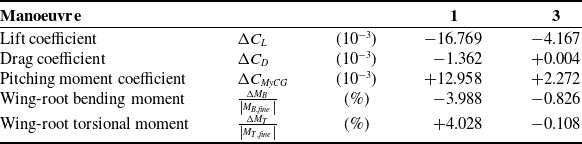
at the wing surface. A comparison of some integral quantities from the original grid solution and from the fine grid solution is presented in Table 5. Here, the deviations between both grids for manoeuvre 3 (
$y^+ < 0.25$
at the wing surface. A comparison of some integral quantities from the original grid solution and from the fine grid solution is presented in Table 5. Here, the deviations between both grids for manoeuvre 3 (
 $\mathrm{M}=0.50$
) are small. However, the deviations for manoeuvre 1 (
$\mathrm{M}=0.50$
) are small. However, the deviations for manoeuvre 1 (
 $\mathrm{M}=0.85$
) are significantly higher and require some discussion.
$\mathrm{M}=0.85$
) are significantly higher and require some discussion.
Table 5. Deviations of the original grid solution from the fine grid solution for manoeuvres 1 and 3

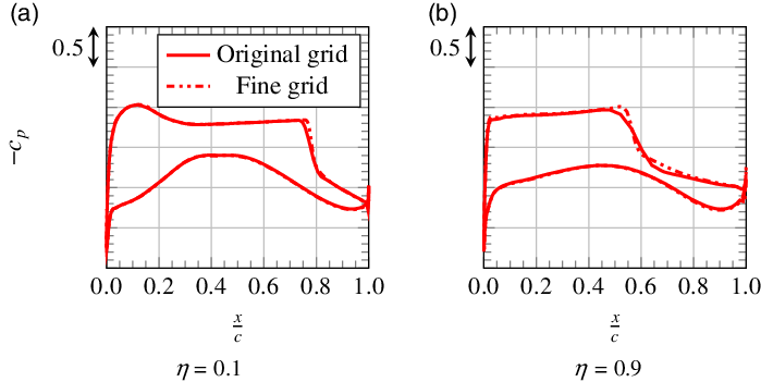
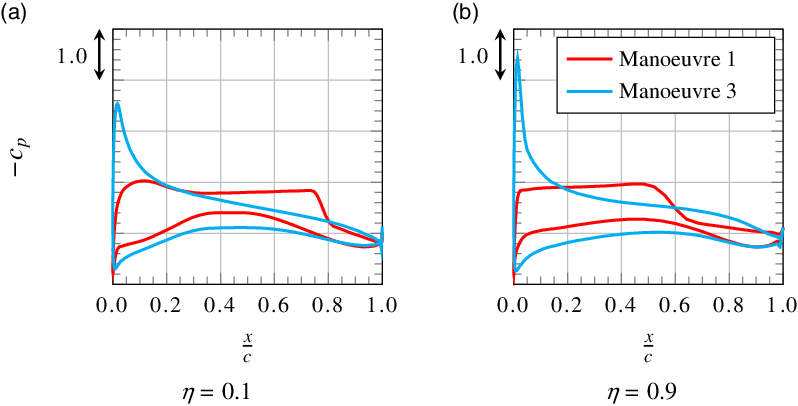
Figure 10 shows the pressure distributions from simulations on both grids at two spanwise positions. At
 $\eta=0.9$
, one can see that the shock is slightly blurred on the original grid, which leads to a lower lift coefficient compared with the fine grid. Comparing the two wing sections at
$\eta=0.9$
, one can see that the shock is slightly blurred on the original grid, which leads to a lower lift coefficient compared with the fine grid. Comparing the two wing sections at
 $\eta=0.1$
and
$\eta=0.1$
and
 $\eta=0.9$
reveals that this effect is much stronger at the outboard wing than at the inboard wing. This explains why the wing-root bending moment is lower for the original grid. Further, it results in an increased pitching moment coefficient for the swept-back wing. Since the shock and consequently the local lift loss are located in the rear region of the wing section, also the higher wing-root torsional moment for the original grid can be explained.
$\eta=0.9$
reveals that this effect is much stronger at the outboard wing than at the inboard wing. This explains why the wing-root bending moment is lower for the original grid. Further, it results in an increased pitching moment coefficient for the swept-back wing. Since the shock and consequently the local lift loss are located in the rear region of the wing section, also the higher wing-root torsional moment for the original grid can be explained.

Figure 10. Pressure distributions at two spanwise positions for manoeuvre 1 from simulations on the original grid and on the fine grid.
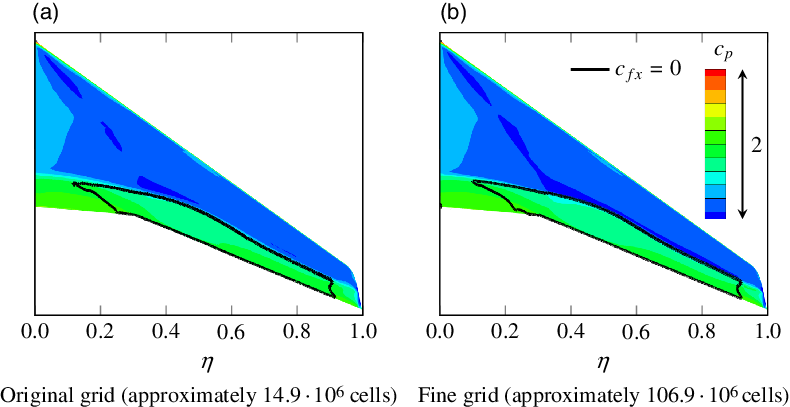
All in all, the deviations are considered to be acceptable here. The goal of this study is not to provide highly accurate numbers that can be used for aircraft design, but rather to present a methodology, allowing for an efficient calculation of flight manoeuvres, and to provide insight into the fundamental physics of manoeuvre loads and load alleviation. And these fundamental flow physics are also captured by the original grid, as shown in Figs 10 and 11. Also, it is important to note that the angle-of-attack was not adjusted for the fine grid simulations. That way, the computational effort is kept at a reasonable level and direct comparability between the CFD simulations on the two grids is achieved. However, if the angle-of-attack were adjusted, this would reduce the differences between the simulations. Here, the angle-of-attack would be reduced for the simulations on the fine grid, as otherwise the lift coefficient and thereby the load factor are too high for the specific manoeuvre.

Figure 11. Pressure distribution and separated regions on the upper surface of the wing for manoeuvre 1 from simulations on the original grid and on the fine grid.
Beyond the issue of grid convergence, also the basic approach of using RANS methods to predict transonic flows near buffet onset needs to be discussed at this point. As no wind-tunnel data for the LEISA aircraft are available, the results from the Sixth AIAA CFD Drag Prediction Workshop summarised by Tinoco et al. [Reference Tinoco, Brodersen, Keye, Laflin, Feltrop, Vassberg, Mani, Rider, Wahls, Morrison, Hue, Gariepy, Roy, Mavriplis and Murayama24] are consulted. For the comparable case of the NASA Common Research model at
 $\mathrm{M}=0.85$
and
$\mathrm{M}=0.85$
and
 $C_L=0.5$
, it is generally confirmed that RANS simulations are capable of capturing the fundamental flow physics observed in wind-tunnel tests, even on coarser grids. Further, the study justifies the neglect of the nacelle and pylon by showing that they have only a small effect on the spanwise distributions of lift and pitching moment.
$C_L=0.5$
, it is generally confirmed that RANS simulations are capable of capturing the fundamental flow physics observed in wind-tunnel tests, even on coarser grids. Further, the study justifies the neglect of the nacelle and pylon by showing that they have only a small effect on the spanwise distributions of lift and pitching moment.
In general, the computed lift is slightly too high and the computed pitching moment is too negative when compared with wind-tunnel experiments. These deviations could partially be related to errors in the reference wind-tunnel data, but the main reason according to Tinoco et al. [Reference Tinoco, Brodersen, Keye, Laflin, Feltrop, Vassberg, Mani, Rider, Wahls, Morrison, Hue, Gariepy, Roy, Mavriplis and Murayama24] is the systematic prediction of excessive aft loading in the simulations. Especially at the outboard wing, the computed pressure distributions show an excessive loading in the rear wing region that leads to an overestimation of lift in those parts of the wing. Based on the fact that most of the participants of the Sixth AIAA CFD Drag Prediction Workshop predicted excessive aft loading, one must assume that this could also be an issue in the present simulations. Here, this would mean that the computed wing bending moments are too high and the computed wing torsional moments are too low.
Further, Tinoco et al. [Reference Tinoco, Brodersen, Keye, Laflin, Feltrop, Vassberg, Mani, Rider, Wahls, Morrison, Hue, Gariepy, Roy, Mavriplis and Murayama24] describe that the shock positions in the simulations become increasingly uncertain at higher angles of attack. This is probably related to buffet, and it is questionable whether steady RANS methods are able to adequately predict the flow in this regime. During the selection of the manoeuvres considered in this study, care was taken to ensure that no buffet occurs in any of them. However, the determination of buffet onset was also based on steady RANS simulations, so this might be a source of uncertainty. Another assumption that might cause some error is the neglect of static aeroelastic deformations of the wing. This aspect is examined further in Section 4.1.
One of the main issues that Tinoco et al. [Reference Tinoco, Brodersen, Keye, Laflin, Feltrop, Vassberg, Mani, Rider, Wahls, Morrison, Hue, Gariepy, Roy, Mavriplis and Murayama24] identified as impairing the validity of RANS simulations is the prediction of premature separation at the junction between wing and fuselage. In the respective simulations, this led to an early lift break compared with wind-tunnel data. However, this does not seem to be a problem in the present simulations as no separation in this specific region and no lift break at low angles of attack are observed.
Although the present simulations might not be accurate enough to use the results in aircraft design, the expected level of uncertainty is considered to be acceptable for the actual purpose of capturing the general trends and understanding the underlying physics.
Quasi-steady simulation
Besides the steady simulations, quasi-steady simulations are performed to investigate the effect of pitching motion on the aerodynamics of the wing–fuselage configuration during the manoeuvre. To identify the angle-of-attack required for a specific, quasi-steady manoeuvre by use of the calculations methods described in Section 3.2, the dynamic derivatives of the model first need to be determined. For this purpose, simulations with and without pitching rate are carried out. From the results, the derivatives are calculated via
 \begin{eqnarray} \frac{\partial \vec{C}_{WF}}{\partial q} = \frac{\Delta \vec{C}_{WF}}{q}\end{eqnarray}
which can be inserted into Equation (9).
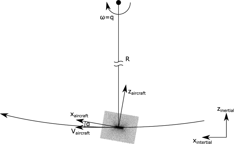
The grid itself remains unchanged in the quasi-steady simulation, but in this application the grid is moved to simulate aircraft motion. As already illustrated in Section 3.2, the trajectory of a pitching manoeuvre can be approximated by a circular path. To reproduce this correctly in the simulations, the grid is suspended at the centre of gravity of the aircraft and moved along a circular path as shown in Fig. 12. Then, the rotational speed
 $\omega$
is equivalent to the pitching rate q. The radius of rotation R is chosen based on the criterion that the inflow velocity resulting from grid rotation equates the desired inflow velocity for the specific manoeuvre.
$\omega$
is equivalent to the pitching rate q. The radius of rotation R is chosen based on the criterion that the inflow velocity resulting from grid rotation equates the desired inflow velocity for the specific manoeuvre.
4.0 Results
4.1 Aerodynamics of the wing–fuselage configuration
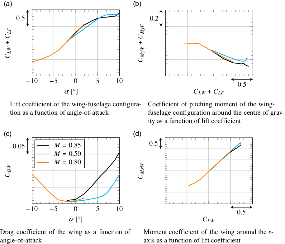
Figure 13 shows the results of steady CFD simulations that were carried out to create a database for the calculation methods discussed in Section 3.2. Three different Mach numbers are considered:
 $\mathrm{M}=0.85$
and
$\mathrm{M}=0.85$
and
 $\mathrm{M}=0.50$
at positive angles of attack, and
$\mathrm{M}=0.50$
at positive angles of attack, and
 $\mathrm{M}=0.80$
at negative angles of attack.
$\mathrm{M}=0.80$
at negative angles of attack.

Figure 12. Grid motion in the quasi-steady simulation of the pitching manoeuvre.

Figure 13. Aerodynamics of the wing–fuselage configuration at different Mach numbers.
Figure 13(a) shows the lift coefficient of the wing–fuselage configuration as a function of angle-of-attack. As expected, the slope of the lift curve
 $\frac{d C_L}{d \alpha}$
is higher for the higher Mach numbers
$\frac{d C_L}{d \alpha}$
is higher for the higher Mach numbers
 $\mathrm{M}=0.85$
and
$\mathrm{M}=0.85$
and
 $\mathrm{M}=0.80$
. The maximum lift coefficient
$\mathrm{M}=0.80$
. The maximum lift coefficient
 $C_{Lmax}$
also behaves as expected and is higher for
$C_{Lmax}$
also behaves as expected and is higher for
 $\mathrm{M}=0.50$
than for
$\mathrm{M}=0.50$
than for
 $\mathrm{M}=0.85$
. The small increase of lift observed at
$\mathrm{M}=0.85$
. The small increase of lift observed at
 $\alpha=10^\circ$
for
$\alpha=10^\circ$
for
 $\mathrm{M}=0.85$
is due to the occurrence of buffet for this case, which cannot be resolved adequately in the steady simulations. This is confirmed by Fig. 14, where the pressure distribution and the separated regions on the upper surface of the wing are shown. At
$\mathrm{M}=0.85$
is due to the occurrence of buffet for this case, which cannot be resolved adequately in the steady simulations. This is confirmed by Fig. 14, where the pressure distribution and the separated regions on the upper surface of the wing are shown. At
 $\alpha=2^\circ$
the flow is partly separated, whereas at
$\alpha=2^\circ$
the flow is partly separated, whereas at
 $\alpha=8^\circ$
the separation area is much larger and slightly fissured, which can be interpreted as indication of the occurrence of unsteady processes. Thus, the results for
$\alpha=8^\circ$
the separation area is much larger and slightly fissured, which can be interpreted as indication of the occurrence of unsteady processes. Thus, the results for
 $\mathrm{M}=0.85$
at high angles of attack are not reliable, and maximum lift in this case is limited by the occurrence of buffet. A similar behaviour is observed for the maximum of negative lift at
$\mathrm{M}=0.85$
at high angles of attack are not reliable, and maximum lift in this case is limited by the occurrence of buffet. A similar behaviour is observed for the maximum of negative lift at
 $\mathrm{M}=0.80$
.
$\mathrm{M}=0.80$
.
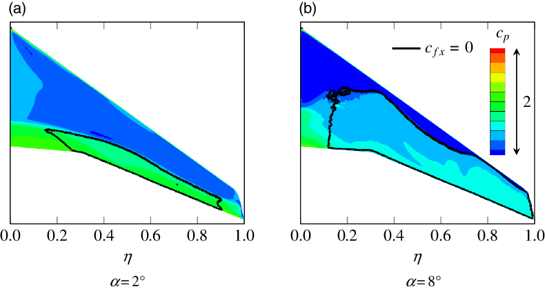
Figure 14. Pressure distribution and separated regions on the upper surface of the wing at different angles of attack for
 $\mathrm{M}=0.85$
.
$\mathrm{M}=0.85$
.
On the contrary, the flow at
 $\mathrm{M}=0.50$
is completely attached for
$\mathrm{M}=0.50$
is completely attached for
 $\alpha=2^\circ$
, as shown in Fig. 15(a). At approximately
$\alpha=2^\circ$
, as shown in Fig. 15(a). At approximately
 $\alpha=5^\circ$
, it becomes transonic and reaches supersonic velocities in the region of the suction peak at the nose. Slightly behind the leading edge, this local supersonic region ends with a shock that becomes stronger with increasing angle-of-attack and causes thickening of the boundary layer. As shown in Figs 15(b) and 16, the adverse pressure gradient behind the suction peak leads to separation at approximately
$\alpha=5^\circ$
, it becomes transonic and reaches supersonic velocities in the region of the suction peak at the nose. Slightly behind the leading edge, this local supersonic region ends with a shock that becomes stronger with increasing angle-of-attack and causes thickening of the boundary layer. As shown in Figs 15(b) and 16, the adverse pressure gradient behind the suction peak leads to separation at approximately
 $\alpha=8^\circ$
, which is also reflected in the increase of drag coefficient in Fig. 13(c). So unlike for
$\alpha=8^\circ$
, which is also reflected in the increase of drag coefficient in Fig. 13(c). So unlike for
 $\mathrm{M}=0.85$
, one observes leading-edge stall that emanates from the midspan region of the wing here. Thus, maximum lift in this case is limited by shock-induced separation.
$\mathrm{M}=0.85$
, one observes leading-edge stall that emanates from the midspan region of the wing here. Thus, maximum lift in this case is limited by shock-induced separation.
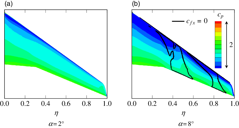
Figure 15. Pressure distribution and separated regions on the upper surface of the wing at different angles of attack for
 $\mathrm{M}=0.50$
.
$\mathrm{M}=0.50$
.
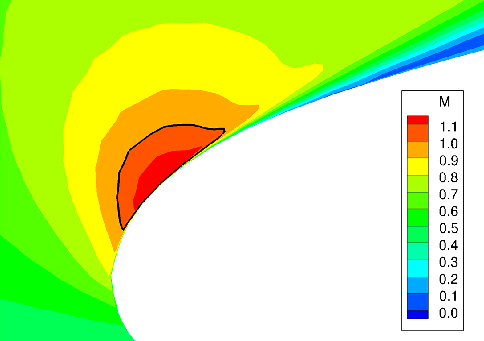
Figure 16. Local Mach number at the leading edge at
 $\eta = 0.456$
for
$\eta = 0.456$
for
 $\alpha = 8^\circ$
and an inflow Mach number of
$\alpha = 8^\circ$
and an inflow Mach number of
 $\mathrm{M} = 0.50$
.
$\mathrm{M} = 0.50$
.
Figure 14(a) indicates that, for
 $\mathrm{M}=0.85$
, separation occurs first at the outer parts of the wing. This has a load alleviating effect that can be identified in Fig. 13(d). Unlike for
$\mathrm{M}=0.85$
, separation occurs first at the outer parts of the wing. This has a load alleviating effect that can be identified in Fig. 13(d). Unlike for
 $\mathrm{M}=0.50$
, the wing moment coefficient around the x-axis
$\mathrm{M}=0.50$
, the wing moment coefficient around the x-axis
 $C_{MxW}$
, which significantly contributes to the wing bending moment, increases less than linearly at high lift coefficients. The impact of this effect is similar to the impact of the elastic torsion of the wing at high Mach numbers described by Hodges et al. [Reference Hodges and McKenzie7]. The latter leads to a reduction of angle-of-attack at the outboard wing and thereby to a reduction of wing bending moment. Hence, neglecting elasticity here results in an overestimation of separation at the outboard wing, but this particular flow phenomenon has a similar outcome in terms of loads.
$C_{MxW}$
, which significantly contributes to the wing bending moment, increases less than linearly at high lift coefficients. The impact of this effect is similar to the impact of the elastic torsion of the wing at high Mach numbers described by Hodges et al. [Reference Hodges and McKenzie7]. The latter leads to a reduction of angle-of-attack at the outboard wing and thereby to a reduction of wing bending moment. Hence, neglecting elasticity here results in an overestimation of separation at the outboard wing, but this particular flow phenomenon has a similar outcome in terms of loads.
The position of the separated regions also has an effect on pitching moment coefficient, as illustrated in Fig. 13(b). Comparing the cases
 $\mathrm{M}=0.85$
and
$\mathrm{M}=0.85$
and
 $\mathrm{M}=0.50$
, the pitching moment coefficient for
$\mathrm{M}=0.50$
, the pitching moment coefficient for
 $\mathrm{M}=0.50$
is found to decrease nearly linearly with lift coefficient until maximum lift is reached, whereas for
$\mathrm{M}=0.50$
is found to decrease nearly linearly with lift coefficient until maximum lift is reached, whereas for
 $\mathrm{M}=0.85$
the moment initially decreases faster and the absolute slope then reduces with increasing lift. Generally, in the transonic region, the neutral point is shifted downstream with increasing Mach number [Reference Schlichting and Truckenbrodt18](pp 176–177). This can also be observed at the inboard wing in Fig. 17, where the local neutral point position is plotted as a function of dimensionless span. At low lift coefficients, this leads to the steeper decrease of pitching moment coefficient for
$\mathrm{M}=0.85$
the moment initially decreases faster and the absolute slope then reduces with increasing lift. Generally, in the transonic region, the neutral point is shifted downstream with increasing Mach number [Reference Schlichting and Truckenbrodt18](pp 176–177). This can also be observed at the inboard wing in Fig. 17, where the local neutral point position is plotted as a function of dimensionless span. At low lift coefficients, this leads to the steeper decrease of pitching moment coefficient for
 $\mathrm{M}=0.85$
. Then, other than for
$\mathrm{M}=0.85$
. Then, other than for
 $\mathrm{M}=0.50$
, flow separates as lift increases. This separation first occurs at the outer and middle parts of the wing, as also shown in Fig. 14(a). Thus, on the swept-back wing, the centre of pressure is shifted upstream. Further, separation emanates from the trailing edge, which leads to an additional upstream shift of the centre of pressure, as shown at the outboard wing in Fig. 17. Eventually, this results in the reduced decrease of pitching moment coefficient at high lift coefficients for
$\mathrm{M}=0.50$
, flow separates as lift increases. This separation first occurs at the outer and middle parts of the wing, as also shown in Fig. 14(a). Thus, on the swept-back wing, the centre of pressure is shifted upstream. Further, separation emanates from the trailing edge, which leads to an additional upstream shift of the centre of pressure, as shown at the outboard wing in Fig. 17. Eventually, this results in the reduced decrease of pitching moment coefficient at high lift coefficients for
 $\mathrm{M}=0.85$
. The curve for
$\mathrm{M}=0.85$
. The curve for
 $\mathrm{M}=0.80$
can be explained in a similar way.
$\mathrm{M}=0.80$
can be explained in a similar way.
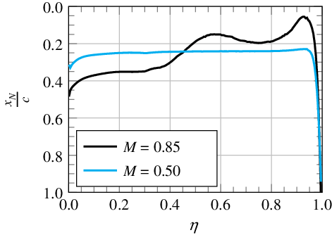
Figure 17. Position of local neutral point as a function of dimensionless span (evaluated between
 $\alpha = 0^\circ$
and
$\alpha = 0^\circ$
and
 $\alpha = 2^\circ$
).
$\alpha = 2^\circ$
).
4.2 Manoeuvre loads from combination of handbook and Navier–Stokes methods
Figure 18 shows the moments at the wing root within the whole flight envelope calculated by combining handbook and Navier–Stokes methods as described in Section 3.2. The flight envelope in this illustration is only limited by maximum lift; other constraints of structural or legal nature as well as limited engine thrust are not considered here. Moments are evaluated for the case of maximum achievable load factor; at the boundary of maximum lift, this is
 $n_z=1$
. With increasing Mach number and decreasing altitude, the achievable load factor increases; at the black line in the diagram, it reaches
$n_z=1$
. With increasing Mach number and decreasing altitude, the achievable load factor increases; at the black line in the diagram, it reaches
 $n_z=2.5$
. Higher manoeuvring load factors are not relevant for commercial aircraft, as already mentioned in Section 2.2. Thus, the load factor at high Mach numbers and low altitudes is limited to
$n_z=2.5$
. Higher manoeuvring load factors are not relevant for commercial aircraft, as already mentioned in Section 2.2. Thus, the load factor at high Mach numbers and low altitudes is limited to
 $n_z=2.5$
. In addition to manoeuvre loads, the three manoeuvres with positive load factor from Table 4 are plotted too.
$n_z=2.5$
. In addition to manoeuvre loads, the three manoeuvres with positive load factor from Table 4 are plotted too.
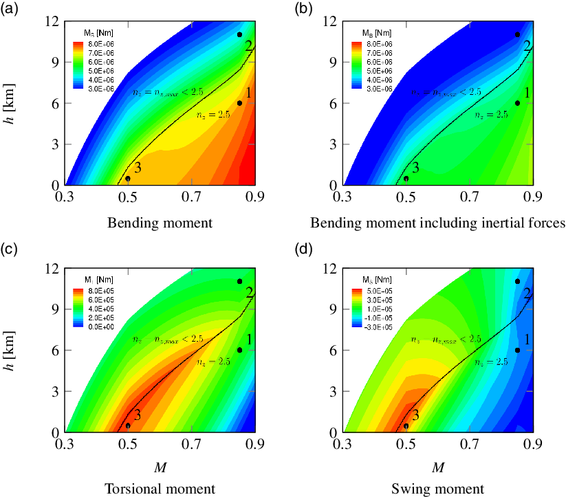
Figure 18. Wing-root loading at maximum load factor within the whole flight envelope from combination of handbook and Navier–Stokes methods.
Comparison between Fig. 18(a) and (b) visualises the load alleviating effect of inertial forces calculated by use of Equation (22). This effect is especially strong at high load factors, as shown in the part of the diagram where
 $n_z=2.5$
. In the part of the diagram where
$n_z=2.5$
. In the part of the diagram where
 $n_z<2.5$
, the angle-of-attack is maximal since the highest achievable load factor should be reached here. With increasing Mach number and decreasing altitude, the stagnation pressure increases and thereby also the achievable load factor as well as the absolute wing-root moments, since the respective aerodynamic coefficients do not change, except for compressibility effects. It is interesting that the swing moment in Fig. 18(d), which is defined positive for swinging forwards (Fig. 7), reaches positive values at low Mach numbers. The reason for this is that the vector of lift relative to the wing rotates forward with increasing angle-of-attack and in consequence pulls the wing forward at high angles of attack. However, with increasing Mach number, the drag coefficient also increases, as illustrated in Fig. 13(c). This leads to a decrease of the swing moment along the
$n_z<2.5$
, the angle-of-attack is maximal since the highest achievable load factor should be reached here. With increasing Mach number and decreasing altitude, the stagnation pressure increases and thereby also the achievable load factor as well as the absolute wing-root moments, since the respective aerodynamic coefficients do not change, except for compressibility effects. It is interesting that the swing moment in Fig. 18(d), which is defined positive for swinging forwards (Fig. 7), reaches positive values at low Mach numbers. The reason for this is that the vector of lift relative to the wing rotates forward with increasing angle-of-attack and in consequence pulls the wing forward at high angles of attack. However, with increasing Mach number, the drag coefficient also increases, as illustrated in Fig. 13(c). This leads to a decrease of the swing moment along the
 $n_z=2.5$
-line. Along this line, the torsional moment decreases as well, as shown in Fig. 18(c). This results from the fact that the neutral point is shifted downstream with increasing Mach number, as mentioned above.
$n_z=2.5$
-line. Along this line, the torsional moment decreases as well, as shown in Fig. 18(c). This results from the fact that the neutral point is shifted downstream with increasing Mach number, as mentioned above.
If the stagnation pressure is further increased starting from the
 $n_z=2.5$
-line, the angle-of-attack decreases since the prescribed load factor remains constant. This leads to a decrease of torsional moment and swing moment, because lift force is acting further downstream on the wing and its vector rotates backwards. The bending moment in this part of the diagram is influenced by many different effects that will be discussed exemplarily on the basis of CFD simulations of specific manoeuvres in the next Section 4.3.
$n_z=2.5$
-line, the angle-of-attack decreases since the prescribed load factor remains constant. This leads to a decrease of torsional moment and swing moment, because lift force is acting further downstream on the wing and its vector rotates backwards. The bending moment in this part of the diagram is influenced by many different effects that will be discussed exemplarily on the basis of CFD simulations of specific manoeuvres in the next Section 4.3.
4.3 Manoeuvre loads from CFD simulations
Comparison of considered manoeuvres
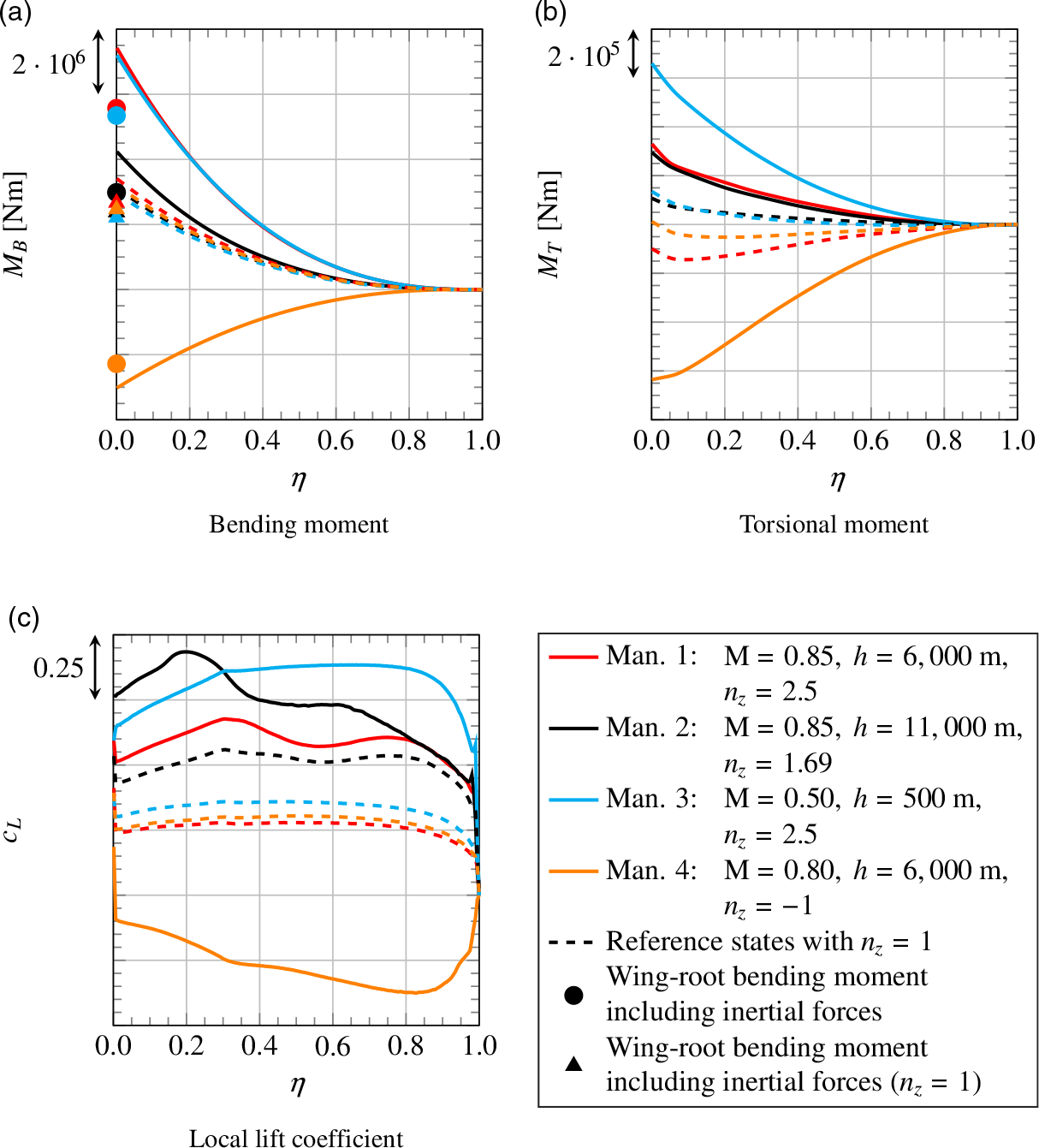
The results from the steady simulations of the considered manoeuvres are illustrated in Fig. 19. Besides bending and torsional moment, the local lift coefficient is shown as a function of dimensionless span. In addition to the actual manoeuvre simulations, reference simulations were performed for steady level flight with
 $n_z=1$
under the respective conditions. For all four reference states, load factor as well as aircraft weight and thereby total lift are equal. Comparing the local lift coefficients in Fig. 19(c) for those cases, one finds that the angle-of-attack is lowest for reference state 1 and highest for reference state 2. Since at low angles of attack the centre of pressure is located further downstream, also the torsional moment in Fig. 19(b) is the lowest for reference state 1. The fact that the torsional moment for reference state 2 is not the highest, although the angle-of-attack is higher than for reference state 3, can be explained with the position of the neutral point, which is located further downstream for the higher Mach number.
$n_z=1$
under the respective conditions. For all four reference states, load factor as well as aircraft weight and thereby total lift are equal. Comparing the local lift coefficients in Fig. 19(c) for those cases, one finds that the angle-of-attack is lowest for reference state 1 and highest for reference state 2. Since at low angles of attack the centre of pressure is located further downstream, also the torsional moment in Fig. 19(b) is the lowest for reference state 1. The fact that the torsional moment for reference state 2 is not the highest, although the angle-of-attack is higher than for reference state 3, can be explained with the position of the neutral point, which is located further downstream for the higher Mach number.

Figure 19. Spanwise wing load distributions for specific manoeuvres and for steady level flight with
 $n_z=1$
under the respective conditions for reference.
$n_z=1$
under the respective conditions for reference.
Although total lift is equal for all four reference states, for the cases with low torsional moment, the tailplane needs to create more negative lift to trim the aircraft. This results in a higher wing loading, as seen in Fig. 19(a), where the bending moment for reference state 1 is the highest, followed by reference states 4 and 2 then 3 with the lowest bending moment.
Examining the four actual manoeuvres, one finds that, for the manoeuvres with positive load factor, bending and torsional moment increase compared with the respective reference states. For the manoeuvre with negative load factor, loads become negative too, but their absolute value is lower than the maximum loads from the manoeuvres with positive load factor. The maximum loads in terms of torsional moment occur for manoeuvre 3 as illustrated in Fig. 19(b). The comparison of pressure distributions for manoeuvre 1 and manoeuvre 3 in Fig. 20 shows that the centre of lift distribution is located further upstream for manoeuvre 3. The reasons for this are the higher angle-of-attack and the neutral point’s being located further upstream for the lower Mach number. Besides, for high Mach numbers, the transonic design of the aerofoil as so-called rooftop-aerofoil with rear loading results in a nearly constant negative pressure coefficient on large parts of the upper surface and high positive pressure coefficients on the rear part of the lower surface. Overall, this leads to a backward shift of the centre of lift distribution for manoeuvre 1. Thus, as for the respective reference states, torsional moment for manoeuvre 3 is higher than for manoeuvre 1. However, other than for the respective reference states, the torsional moment for manoeuvre 2 is not on the same order of magnitude as for manoeuvre 3, but much lower. This results from the lower load factor. The lower load factor also explains why the bending moment in Fig. 19(a) is much lower for manoeuvre 2 than for manoeuvres 1 and 3.

Figure 20. Pressure distributions at two spanwise positions for manoeuvres 1 and 3.
When comparing the bending moment for manoeuvres 1 and 3, one finds an approximately 3% higher value at the wing root for manoeuvre 1. However, in the middle region of the wing, the bending moment for manoeuvre 3 is slightly higher. This behaviour is caused by different effects that will be addressed in the following.
As already mentioned, the torsional moment for manoeuvre 3 is much higher than for manoeuvre 1. As a consequence, during manoeuvre 1, the tailplane needs to create more negative lift and thus the wing needs to create more positive lift. Even though this additional lift increases the bending moment, the centre of the respective spanwise lift distribution in Fig. 19(c) is located further inboard, thus having an alleviating effect on the bending moment. The reason for the different lift distributions is that flow separates for manoeuvre 1, as illustrated in Fig. 21. One can see that flow is only separated in the middle and outer regions of the wing, whereas for manoeuvre 3 flow is completely attached. This is confirmed by the pressure distributions in Fig. 20. Finally, this explains why the bending moment for manoeuvre 1 is higher than for manoeuvre 3 at the wing root whereas in the middle and outer regions of the wing the opposite is true.
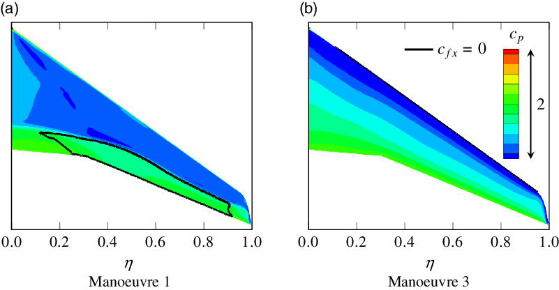
Figure 21. Pressure distribution and separated regions on the upper surface of the wing for manoeuvres 1 and 3.
In addition to the aerodynamic bending moments, Fig. 19(a) also shows the wing-root bending moments that result from additionally considering inertial forces. Like in Fig. 18, one observes a strong load alleviating effect that is especially significant for high absolute load factors.
Effect of pitching motion
The effect of pitching motion on the aerodynamics of the wing–fuselage configuration is illustrated in Fig. 22. Here the results from steady and quasi-steady simulations are compared. For this, manoeuvre 3 is chosen, as it features the highest pitching rate as well as the highest dimensionless pitching rate
 $\frac{q \cdot MAC_W}{V}$
among all the manoeuvres.
$\frac{q \cdot MAC_W}{V}$
among all the manoeuvres.
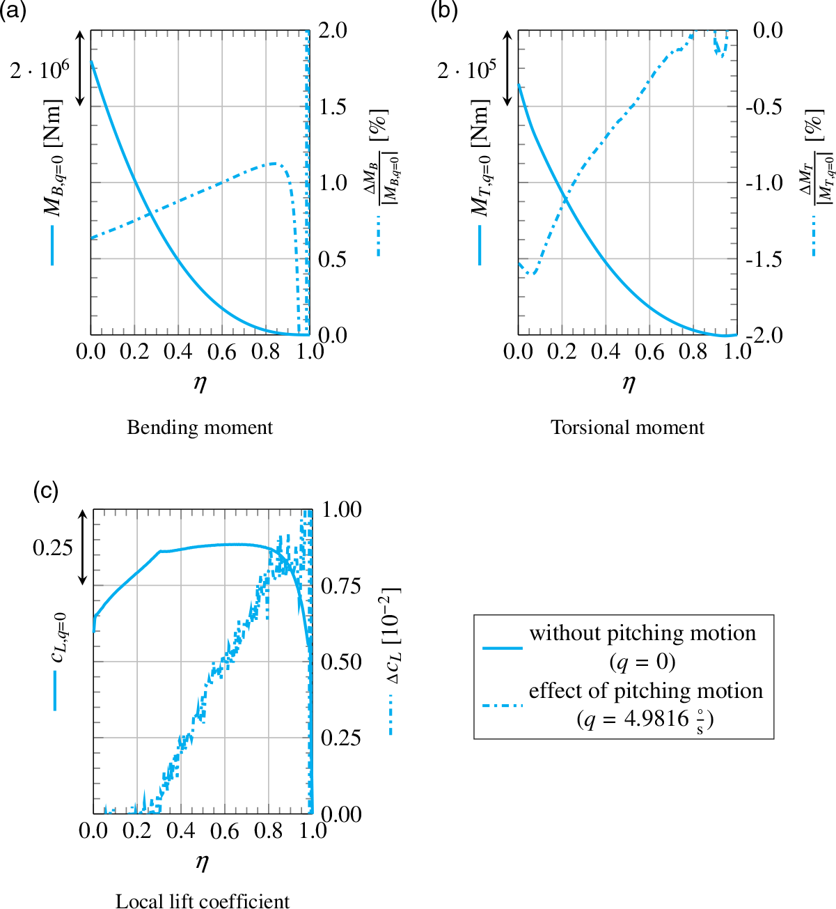
Figure 22. Effect of pitching motion on spanwise wing load distributions for manoeuvre 3.
The main effect of pitching motion is that it changes the distribution of angle-of-attack. Upstream of the centre of gravity, the local angle-of-attack is reduced, while downstream of the centre of gravity it is increased. This results in an additional, negative torsional moment as shown in Fig. 22(b). As a consequence, the tailplane needs to create more negative lift and the wing loading increases, as illustrated in Fig. 22(c). This also leads to a higher bending moment in Fig. 22(a). The increase in bending moment is augmented by the effect that, for a swept-back wing, the changed distribution of angle-of-attack results in an additional loading of the outboard wing, which is also shown in Fig. 22(c).
However, all in all, the deviations between the steady and quasi-steady simulation are small. The difference in wing-root bending moment is only
 $0.63\%$
, while the difference in wing-root torsional moment is
$0.63\%$
, while the difference in wing-root torsional moment is
 $-1.53\%$
. Hence, the effect of pitching motion on the aerodynamics of the wing–fuselage configuration can be neglected.
$-1.53\%$
. Hence, the effect of pitching motion on the aerodynamics of the wing–fuselage configuration can be neglected.
Load alleviation
As described in Section 2.1, the load alleviation system for the LEISA configuration uses a droop nose divided into five segments at the leading edge and four plain flaps and the aileron at the trailing edge. However, in a first step, only the outer trailing-edge flap and the aileron are considered here. Both are negatively deflected to reduce lift at the outboard wing and thereby the bending moment. Similar concepts were successful in studies performed by Disney [Reference Disney8] for a Lockheed C-5A Galaxy and by White [Reference White11].
At this point, one of the previously discussed manoeuvres is chosen to evaluate the potential of load alleviation for this case. Here, the critical manoeuvres are manoeuvres 1, 3 and 4. Since only control surfaces at the outboard wing are considered, the reduced lift needs to be compensated by an increase of angle-of-attack to reach the required load factor. For manoeuvres 3 and 4, the wing operates close to its aerodynamic limit so a further increase of angle-of-attack would lead to separation. Hence, manoeuvre 1 is chosen here. If load alleviation is sought for manoeuvres 3 and 4 without compromising manoeuvrability, the inboard control surfaces must be used to increase lift locally.
The outer trailing-edge flap and aileron are deflected by an angle of
 $\xi=-15^\circ$
. This value is an estimation based on typical maximum aileron deflections of large transport aircraft. For the simulations, the gaps between the deflected control surfaces and the wing are closed by linear blending and thereby neglected.
$\xi=-15^\circ$
. This value is an estimation based on typical maximum aileron deflections of large transport aircraft. For the simulations, the gaps between the deflected control surfaces and the wing are closed by linear blending and thereby neglected.
The spanwise distributions of bending moment, torsional moment and local lift coefficient are compared in Fig. 23 for the steady simulation of manoeuvre 1 with and without load alleviation. Here also, the respective reference state with
 $n_z=1$
is plotted. Furthermore, Fig. 23(c) and (d) show the bending moments and the torsional moments relative to this reference state. The pressure distributions and the separated regions on the wing surface are illustrated in Fig. 24, while Fig. 25 shows the pressure distributions at two specific wing sections located at the two flaps.
$n_z=1$
is plotted. Furthermore, Fig. 23(c) and (d) show the bending moments and the torsional moments relative to this reference state. The pressure distributions and the separated regions on the wing surface are illustrated in Fig. 24, while Fig. 25 shows the pressure distributions at two specific wing sections located at the two flaps.

Figure 23. Spanwise wing load distributions for manoeuvre 1 with and without load alleviation and for steady level flight with
 $n_z=1$
under the respective conditions for reference.
$n_z=1$
under the respective conditions for reference.

Figure 24. Pressure distribution and separated regions for manoeuvre 1 with and without load alleviation.
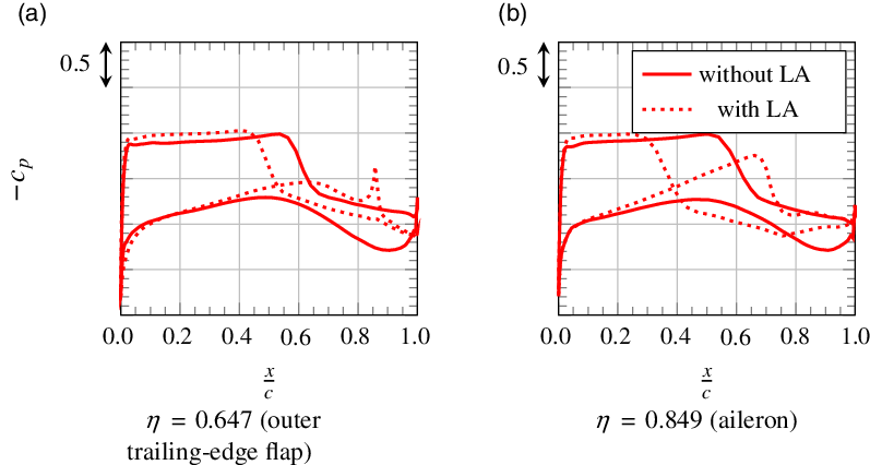
Figure 25. Pressure distributions at two spanwise positions for manoeuvre 1 with and without load alleviation.
The primary effect of the negatively deflected flaps is depicted in Fig. 23(e). The outboard wing is unloaded in the region of the flaps, but the local lift coefficient does not become negative here. This is explained by the fact that flow is separated on large parts of the lower flap side, as shown in Fig. 24(c). Especially on the aileron, a large region of separation is found, as confirmed by the respective pressure distribution in Fig. 25(b). The reason for separation occurring especially on the aileron and not on the plain flap is the greater size of the aileron (Fig. 2). Thus, the hinge line is located further upstream in a region where, even with no aileron deflection, an adverse pressure gradient exists on the lower wing surface. This augments the pressure increase immediately behind the hinge line induced by deflecting the aileron and eventually the boundary layer separates. Comparison with the pressure distribution on the plain flap in Fig. 25(a) shows that the hinge line of the plain flap is located in a region where, without flap deflection, only a small pressure gradient exists on the lower wing surface. Hence, the boundary layer is less prone to separate here.
The fact that the aileron is larger than the plain flap also explains why the strongest reduction of lift coefficient can be observed at the aileron.
As mentioned above, the lift reduction at the outboard wing is compensated by an increase of the angle-of-attack so that the lift at the inboard wing is increased. When comparing the spanwise lift distributions for the cases with and without load alleviation in Fig. 23(e) and determining the total lift coefficients, one must consider that the local lift coefficients are normalised using the local wing chord. Thus, the lift coefficients at the inboard wing are weighted more strongly and the difference in total lift is less than appears in the figure. However, even considering this fact, one obtains a total lift coefficient that is more than 8% lower for the wing with load alleviation. The reason for this is that the tailplane needs to generate less negative lift since the torsional moment of the wing is significantly increased by applying load alleviation. Figure 23(b) and (d) reveals considerable differences in torsional loads already at the outboard wing. These arise from the fact that the negatively deflected flaps lead to an increase of zero-lift moment that is also apparent from the pressure distributions shown in Fig. 25. The pressure distributions further indicate that the higher angle-of-attack for the case with load alleviation causes lower pressure in the front region of the upper wing surface. As also shown in Fig. 24, this leads to separation further upstream, and as a consequence, the torsional moment is further increased.
In Fig. 23(a), the bending moment is plotted as a function of dimensionless span. Especially at the outboard wing, it is significantly reduced by load alleviation. But also at the wing root the value is about 33% lower. Considering the effect of inertial forces, the reduction in wing-root bending moment seems to be even larger with a value of 44%. As shown in Fig. 23(c), the wing-root bending moment is then only 18% higher than for the respective reference state with
 $n_z=1$
. It appears that the optimisation of the combination of different control surface deflections provides the potential to reduce loads even further. However, this may not even be necessary for the manoeuvre discussed here. Ramsey et al. [Reference Ramsey and Lewolt9] and White [Reference White11] state that, regarding the structural design of the wing, manoeuvre loads are rather relevant for the middle and outer parts of the wing but not for the inner parts. And, as is also apparent from Fig. 23(c), the bending moment in those middle and outer parts of the wing is actually lower than for the respective reference state, sometimes by even more than 75%. The corresponding effect on the wing structure should be examined in further studies, taking into account the detailed structural design of the LEISA configuration. Then, also the effect of the increased torsional moment needs to be evaluated.
$n_z=1$
. It appears that the optimisation of the combination of different control surface deflections provides the potential to reduce loads even further. However, this may not even be necessary for the manoeuvre discussed here. Ramsey et al. [Reference Ramsey and Lewolt9] and White [Reference White11] state that, regarding the structural design of the wing, manoeuvre loads are rather relevant for the middle and outer parts of the wing but not for the inner parts. And, as is also apparent from Fig. 23(c), the bending moment in those middle and outer parts of the wing is actually lower than for the respective reference state, sometimes by even more than 75%. The corresponding effect on the wing structure should be examined in further studies, taking into account the detailed structural design of the LEISA configuration. Then, also the effect of the increased torsional moment needs to be evaluated.
Besides the primary effects on wing loads, additional, secondary effects of load alleviation are identified. As mentioned above, the loads on the tailplane are also reduced. Hence, weight savings are conceivable here too. Further, reduced loads on the tailplane also involve a reduced fuselage bending moment. On the other hand, it may be disadvantageous regarding roll authority if the ailerons are used for load alleviation at high load factors. Those secondary effects should also be considered in future studies.
5.0 Conclusions
The goal of this study is to identify critical manoeuvres in terms of wing loads, develop methods to predict those loads and evaluate the potential of a load alleviation system applied to the LEISA research configuration, a large generic transport aircraft with a swept-back wing. Four exemplary pitching manoeuvres were chosen based on the CS-25 regulations. For the calculation of those manoeuvres, handbook and Navier–Stokes methods were combined and only the quasi-steady phase of the manoeuvre was considered. Unsteady processes during initiation of the manoeuvre were neglected, as well as aeroelastic effects. In addition, one particular manoeuvre with high, positive load factor at high Mach number was calculated with active load alleviation. Here, the aileron and a plain flap at the outboard wing were negatively deflected. As a result, the wing-root bending moment for the rigid wing could be reduced by 44%, reducing it to a value only 18% higher than for steady level flight with
 $n_z=1$
under the respective flight conditions.
$n_z=1$
under the respective flight conditions.
The results further indicate which manoeuvres are critical regarding loads and load alleviation. This is of major importance for future studies. The following four manoeuvres are suggested for consideration in further investigations:
A pitching manoeuvre with
$n_z=2.5$
at
$\mathrm{M}=\mathrm{M}_A$
and at
$h=0\;\text{m}$
generates high bending moments as well as high torsional moments. The torsional moment is further increased by load alleviation, raising the question of whether this leads to weight penalties in wing structure design. Moreover, the wing operates close to its aerodynamic limit. Hence, a lift reduction at the outboard wing cannot be compensated by an increase of angle-of-attack. Instead, control surfaces at the inboard wing must be used to increase lift locally.A pitching manoeuvre with
$n_z=2.5$
at
$\mathrm{M}=\mathrm{M}_A=\mathrm{M}_{MO}$
and at the respective altitude also generates high bending moments. The aerodynamic wing loading is maximal here too. In addition, further difficulties may be introduced as the load alleviation potential at the high Mach number might be restricted by buffet. Another challenge might be that flap effectiveness decreases with increasing Mach number.A nose-down pitching manoeuvre with
$n_z=-1$
at the lowest possible Mach number and at
$h=0\text{m}$
results in high negative bending and torsional moments. Moreover, bending moment deviations from steady level flight with
$n_z=1$
are maximal, which may be challenging for the load alleviation system, especially since the aerodynamic wing loading is maximal here too.In addition to symmetrical manoeuvres, it would be interesting to consider rolling manoeuvres too. In combination with high load factors, this also raises the question of whether load alleviation and roll authority conflict with each other. In those studies, not only the quasi-steady manoeuvre but also the case with maximum rolling acceleration should be investigated.


Another question that needs to be answered in this context is how the manoeuvrability of the aircraft may be influenced by the load alleviation system. On this basis, different combinations of control surface deflections can be evaluated and optimised regarding load alleviation and their effects on manoeuvrability. Aeroelastic effects should then also be taken into account, since they might have a strong impact on loads and the separation observed at the outboard wing for some cases. In addition, they affect flap effectiveness, especially at the outboard wing, and thereby the effectiveness of the load alleviation system. Those investigations require coupled aerostructural simulations that could subsequently also be used to examine the effect of inertial forces on the spanwise distribution of manoeuvre loads. Since the mass distribution of the wing plays an important role here, it is advisable also to consider different loading conditions for the different manoeuvres.
To quantify possible weight savings, information regarding the structural design of the LEISA configuration is required. It must be analysed how the structure can be modified depending on maximum loads and how this eventually affects the weight and efficiency of the aircraft. Finally, the benefits of applying load alleviation can be evaluated. The results presented herein provide a promising basis for such future studies.
Acknowledgments
The authors are grateful for the support of several individuals. Wolfgang Heinze (TU Braunschweig) and Jochen Wild (DLR) provided data for the LEISA aircraft and some useful advice, Lorenz Klug (TU Braunschweig) supported the execution of the CFD simulations and André Bauknecht (TU Braunschweig) made many suggestions that improved the quality of the language in this manuscript. Also, funding by the Bundesministerium für Wirtschaft und Energie within the scope of the Luftfahrtforschungsprogramm VI-1 project INTELWI-TUBS (funding identifier 20A1903J) is gratefully acknowledged.