2.1 Energy scaling law

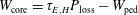Figure 1. Plasma energy content is decomposed between offset ( $W_{o}$ ), pedestal ( $W_{\text{ped}}$ ) and core ( $W_{\text{core}}$ ). The core energy is defined as $W_{\text{core}}=\unicode[STIX]{x1D70F}_{E,L}P_{\text{loss}}$ in low confinement mode (L-mode) and $W_{\text{core}}=\unicode[STIX]{x1D70F}_{E,H}P_{\text{loss}}-W_{\text{ped}}$ in H-mode with $W_{\text{ped}}=\unicode[STIX]{x1D70F}_{E,\text{ped}}P_{\text{loss}}$ .

Various scaling laws based on simple models are used in the METIS code. Scaling laws used for energy content prediction that depend on the scenarios are paired (cf. figure 1): one for the L-mode and one for the H-mode, or one for the pedestal energy and one for the total H-mode energy. The energy content, linked to the confinement time, is given by

where $P_{\text{loss}}$ is the plasma loss power and $\unicode[STIX]{x1D70F}_{\text{sc},\ldots }$ is the energy confinement time with the subscript ‘ $\text{sc},\ldots$ ’ denoting the energy scaling laws for different types of confinement regime in the METIS code. In this paper, for example, the energy confinement time law ITERL-96 ( $\unicode[STIX]{x1D70F}_{E,L}$ ) and ITERH-98( $y,2$ ) ( $\unicode[STIX]{x1D70F}_{E,H}$ ) (Wakatani et al. Reference Wakatani, Mukhovatov, Burrell, Connor, Cordey, Esipchuk, Garbet, Lebedev, Mori and Toi1999) are adopted separately for L-mode and H-mode, while the pedestal energy confinement time takes the form $\unicode[STIX]{x1D70F}_{\text{ped}}=(\unicode[STIX]{x1D70F}_{E,L}+\unicode[STIX]{x1D70F}_{E,H})/2$ and gives quite reasonable results.

In practice, the plasma confinement can be modified by various processes, and in METIS we ultimately rewrite the (2.1) as follows:

where $W_{\text{ITB}}=(H_{\text{ITB}}-1)\unicode[STIX]{x1D70F}_{E,\text{sc}}W_{\text{core}}$ . $H_{\text{ref}}$ is a prescribed factor according to the characterizing feature of tokamak discharge, and $H_{\text{MHD}}$ and $H_{\text{ITB}}$ are internally computed, time-dependent, confinement factors that take into account the confinement degradation due to MHD effects or confinement enhancement due to the formation of internal transport barriers (ITBs). By default, all these multiplicative factors are equal to 1, equation (2.2) can thus reduce to the simple form of (2.1).

The transition from L-mode to H-mode requires that the total input power $P_{\text{in}}$ is greater than the H-mode power threshold $P_{\text{thr}}$ , which is given by the empirical scaling LH99(1) as follows (Snipes & Database Reference Snipes and Database2000):

where $S$ is the plasma external surface area, and $n_{e,\text{bar}}$ and $m_{i}$ are line-averaged electron density and atomic mass number, respectively. In addition, the offset power may be required to fit the experimental data of EAST (Liu et al. Reference Liu, Gao, Liu, Ding, Xia, Zhang, Zhang, Wang, Han and Li2013).

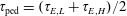
In METIS, the pressure $P_{\text{ped}}$ at the top of the pedestal is computed with the energy content predicted by scaling law and modulated by a free coefficient  $f_{\text{ped}}$ :

where $W_{\text{ped},\text{sc}}=P_{\text{loss}}\times \unicode[STIX]{x1D70F}_{\text{ped},\text{sc}}$ and by default $f_{\text{ped}}$ is set to 1.

2.2 Profiles description

The density profile ( $n_{e,x}$ ) is described by the line-averaged value ( $n_{e,\text{bar}}$ ), the peaking factor ( $\unicode[STIX]{x1D708}_{n}$ ) and the edge density value ( $n_{e,a}$ ) obtained from a simple model. In L mode, the shape of the density profile takes the following form:

where $\unicode[STIX]{x1D708}_{n}=n_{e,a}/n_{e,\text{bar}}$ . In H mode, the density profile is computed by another method to ensure that the pedestal is also present. The density profile is constrained by the given volume averaged value, the peaking factor and the constraint of zero derivative at the centre. The edge value is obtained separately, and then, the other point value is derived by using cubic Hermite polynomial interpolation.

The temperature profiles are computed using time-independent transport equations:

where $Q_{e}$ and $Q_{i}$ are the total heat sources for electrons and ions respectively, as defined in CRONOS (Artaud et al. Reference Artaud, Basiuk, Imbeaux, Schneider, Garcia, Giruzzi, Huynh, Aniel, Albajar and Ane2010), $\unicode[STIX]{x1D705}_{e}=\unicode[STIX]{x1D705}_{0}(1+K_{E}x^{2})$ and $\unicode[STIX]{x1D705}_{i}=\unicode[STIX]{x1D707}_{e,i}\unicode[STIX]{x1D705}_{e}$ are electron and ion heat diffusivity coefficients shape with $\unicode[STIX]{x1D707}_{e,i}$ computed with the help of Ion Temperature Gradient and Trapped Electron Mode (ITG-TEM) fluid stability analysis (Asp et al. Reference Asp, Weiland, Garbet, Mantica, Parail, Suttrop and Contributors2005), $K_{E}$ is a shape scalar factor to fit the experiment data, and $\unicode[STIX]{x1D705}_{0}$ is a constant normalized to retrieve the correct energy content. In addition, the heat diffusivity coefficients shape will be rewritten, when the ITB forms, as (Waltz et al. Reference Waltz, Staebler, Dorland, Hammett, Kotschenreuther and Konings1997):

with $f_{s}(q,\unicode[STIX]{x1D6FC})=\text{e}^{-(s-(3/5)\unicode[STIX]{x1D6FC}-(1/2))^{2}/2}$ , where $s=(x/q)(\text{d}q/\text{d}x)$ and $\unicode[STIX]{x1D6FC}=-Rq^{2}(\text{d}\unicode[STIX]{x1D6FD}/\text{d}x)$ with $\unicode[STIX]{x1D6FD}=2\unicode[STIX]{x1D707}_{0}P/B^{2}$ ( $P$  is the total pressure), $\bar{q}$ is the monotonic safety factor given by $\bar{q}=\min (q)+x^{\unicode[STIX]{x1D710}_{q}}(q(x=1)-\min (q))$ and $\unicode[STIX]{x1D710}_{q}$ is computed to minimized $\int _{x_{\text{min}}}^{1}(q-\bar{q})^{2}\,\text{d}x$ with $x_{\text{min}}$ is the most external position where $q=\min (q)$ . The ITB mechanism is based on the magnetic shear effect and the Shafranov shift effect (Garbet et al. Reference Garbet, Mantica, Angioni, Asp, Baranov, Bourdelle, Budny, Crisanti, Cordey and Garzotti2004), and the effect of ITB is separated into two consistent parts: the first is the increase of the plasma energy content by the modification of the $H_{\text{ITB}}$ parameter (cf. (2.2)), and the second is the change in the transport coefficient shape (cf. (2.7)).

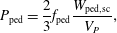
The edge value of density and temperature are necessary to solve the equations for the density and temperature profiles. In H-mode with divertor configurations, the edge density is given by the adapted multi-machine law $n_{e,a}=(5\times 10^{-21}{-}6.7\times 10^{-24}T_{e,a})n_{\text{min}}^{2}$ with $n_{\text{min}}=\min (n_{e,\text{bar}},n_{Gr})$ (Mahdavi et al. Reference Mahdavi, Maingi, Groebner, Leonard, Osborne and Porter2003), where $T_{e,a}$ is the edge electron temperature, $n_{Gr}$ is the Greenwald limit density; In L-mode plasma, the scaling law 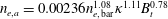$n_{e,a}=0.00236n_{e,\text{bar}}^{1.08}\unicode[STIX]{x1D705}^{1.11}B_{t}^{0.78}$ is used (Porter et al. Reference Porter, Davies, Labombard, Loarte, McCormick, Monk, Shimada and Sugihara1999), where $\unicode[STIX]{x1D705}$ is the plasma elongation and $B$ is the toroidal magnetic field. In addition, for edge temperature in H-mode, the model $T_{e,a}=1.18\times 10^{-7}T_{e,d}^{0.2}(n_{e,a}L_{c}(1-f_{\text{sol}}/2))^{0.4}$ is used (Erents et al. Reference Erents, Stangeby, Labombard, Elder and Fundamenski2000), where $L_{c}$ is the flux tube’s connection length, $f_{\text{sol}}=P_{\text{rad},\text{SOL}}/P_{\text{loss}}$ is the fraction of radiative power loss in the scrape-off layer (SOL) and $T_{e,d}=15(1+f_{\text{pellet}})$ is the divertor temperature with $f_{\text{pellet}}$ is the fraction of fuelling coming from pellet injection. In L mode, the edge temperature is given by $T_{e,a}=(P_{\text{LCMS}}/en_{e,a}\unicode[STIX]{x1D6FE}_{tr}L_{c}^{2}\unicode[STIX]{x1D706}_{\text{SOL}}C_{s})^{2/3}$ , where $P_{\text{LCMS}}$ is the power convected to the separatrix, $C_{s}$ is the sound speed, $\unicode[STIX]{x1D6FE}_{tr}=7$ is the sheath heat transmission coefficient, and $\unicode[STIX]{x1D706}_{\text{SOL}}$ is the characteristic SOL decay length (Stangeby Reference Stangeby2000).

2.3 Heating and current driven

The description of the sources is very important in order to obtain precise predicted values. The sources are decomposed into total power, total current drive, profile power source and current profile source. Each of these terms is computed with different formulations, depending on the best methods available (in terms of computing speed and precision).

The NBI is described by a decay equation applied in a simplified geometry and an analytical solution of the Fokker–Planck equation. The beam intensity damping equation along the beam path is $\text{d}\unicode[STIX]{x1D6FE}/\text{d}\unicode[STIX]{x1D704}=-n_{e}(\unicode[STIX]{x1D704})\unicode[STIX]{x1D70E}_{\text{eff}}(\unicode[STIX]{x1D704})\unicode[STIX]{x1D6FE}(\unicode[STIX]{x1D704})$ , where $\unicode[STIX]{x1D704}$ is the coordinate along the beam path with initial condition $\unicode[STIX]{x1D6FE}(\unicode[STIX]{x1D704}=0)=\unicode[STIX]{x1D6FE}_{0}$ at the entrance of the plasma and $\unicode[STIX]{x1D70E}_{\text{eff}}$ is the effective stopping cross-section depending on the beam ion mass ( $A_{b}$ ), the initial beam energy ( $E_{b}(x=0)$ ), the plasma effective charge ( $Z_{\text{eff}}$ ), the electron density ( $n_{e}$ ) and temperature ( $T_{e}$ ), etc. (Janev, Boley & Post Reference Janev, Boley and Post1989). Combining the decay equation and the orbit width $\unicode[STIX]{x1D6FF}$ (Eriksson & Porcelli Reference Eriksson and Porcelli2001), the power deposition ( $p_{b}(x)$ ) and the broadening of the deposition profile can be simulated. From the power deposition, the fraction of the power that heats the main plasma ions can be computed by using the formulae (5.4.12) in Wesson (Reference Wesson2011a ). The current source associated with NBI is computed by $J_{\text{NBI}}^{\text{fast}}=e(p_{b}(x)/E_{b}(x))\unicode[STIX]{x1D70F}_{s}\unicode[STIX]{x1D709}_{b}((v_{0}^{3}+v_{c}^{3})/v_{0}^{3})^{2v_{\unicode[STIX]{x1D6FE}}^{3}/3v_{0}^{3}}\int _{0}^{v_{0}/v_{c}}(z^{3}/(z^{3}+1))^{(2v_{\unicode[STIX]{x1D6FE}}^{3}/3v_{0}^{3})+1}\,\text{d}z$ , where $\unicode[STIX]{x1D70F}_{s}$ is the slowing down time, $v_{c}$ and $v_{\unicode[STIX]{x1D6FE}}$ are critical velocities and $v_{0}$ is the fast ions’ initial velocity defined in the Stix paper (Stix Reference Stix1975).

In minority heating of ICRF scheme, a fast ion population is generated and heats the majority plasmas. This means that good knowledge of the fast ion distribution function is essential. The analytical Stix formulation (Stix Reference Stix1975) that gives the steady-state velocity distribution function $f(v)$ without space dependence is used in METIS. This distribution function $f(v)$ is computed for each time and all involved parameters are taken at the resonance position $R_{\text{res}}(t)$ on the equatorial plane. The resonance position $R_{\text{res}}(t)$ and the harmonic are computed from the magnetic equilibrium, taking into account the ICRF frequency, the minority ion mass, charge and concentration. Since the hydrogen resonance coincides with the seconded harmonic resonance of deuterium, both the hydrogen ions and the deuterium ions will absorb the wave power at the same location and so, the fraction absorbed by the hydrogen is a key parameter. This fraction is deduced from the resonance width scaled on the PION code results (Eriksson, Hellsten & Willen Reference Eriksson, Hellsten and Willen1993). In addition, the shape of the ICRF power deposition is assumed to be a Gaussian curve centred on the resonance position, with a width proportional to the resonance width.

Figure 2. Graph of absorption for lower hybrid wave. $\unicode[STIX]{x1D6E4}_{L}$ is the Landau damping condition (black line); $N_{\text{acc}}=\sqrt{S}+\sqrt{D^{2}/|P|}$ is the accessibility limit (red line); $\unicode[STIX]{x1D6EC}_{\text{low}}=n_{\Vert 0}/(1+(\unicode[STIX]{x1D70C}/qR_{\text{axe}})\sqrt{-P/S})$ and $\unicode[STIX]{x1D6EC}_{\text{low}}=n_{\Vert 0}/(1-(\unicode[STIX]{x1D70C}/qR_{\text{axe}})\sqrt{-P/S})$ are lower and higher caustic (green line), where $q$ is the safety factor, $\unicode[STIX]{x1D70C}$ is the normalized radius, $R_{\text{axe}}$ is the geometrical axes of each flux surface, $S$ and $P$ are the elements of Stix dielectric tensor.

A semi-analytic model is used to describe the LHCD effect, and is separated into two parts. The first part consists of the computation of the current source profile. The second part is the evaluation of the scaling law for LHCD-driven efficiency or a simple law deduced for the C3PO/LUKE simulations (Peysson & Shoucri Reference Peysson and Shoucri1998). The power deposition is taken proportional to the current source and only electrons are heated. The lower hybrid (LH) power damping model adopted in METIS is a heuristic model that is based on the statistical theory developed by Kupfer and Moreau (Kupfer & Moreau Reference Kupfer and Moreau1992; Kupfer, Moreau & Litaudon Reference Kupfer, Moreau and Litaudon1993). In the METIS description, the $n_{\Vert }$ bounds that are allowed by the dispersion relation are referred to as upper caustics ( $\unicode[STIX]{x1D6EC}_{\text{high}}$ ) and lower caustics ( $\unicode[STIX]{x1D6EC}_{\text{low}}$ ), and the limit of the Landau damping is called $\unicode[STIX]{x1D702}_{L}$ (shown in figure 2). The strong Landau damping is given roughly by $n_{\Vert \text{abs}}=6.5/\sqrt{T_{e}(\text{keV})}$ . Mainly, the power deposition is computed using the distance between local Landau damping condition $\unicode[STIX]{x1D6E4}_{L}$ and local wave $n_{\Vert }$ . This distance, normalized to spectrum width, is the argument for a Gaussian function. Additionally, the power deposition decreases when wave $n_{\Vert }$ is approaching the caustic curves and accessibility condition $N_{\text{acc}}$ . The modified form of the power and current source shape are thus:

where $\unicode[STIX]{x1D712}$ is the penalization of absorption probability due to caustic propagation and accessibility limit (J. Artaud, private communication). $\unicode[STIX]{x1D6FF}n$ is defined as $\unicode[STIX]{x1D6FF}n_{0}(n_{\Vert \text{abs}}/n_{\Vert 0})$ with $n_{\Vert 0}$ is the initial refraction index of wave spectrum and $\unicode[STIX]{x1D6FF}n_{0}$ is initial width of wave spectrum. $n_{\Vert \text{abs}}$ corresponds to the position where strong Landau damping occurred.

Once the LH power absorption profile is computed, the driven current is determined from the current efficiency, as follows:

where $\unicode[STIX]{x1D702}_{\text{LH}}$ is LH efficiency given either by the scaling law or prescribed. For $V_{\text{loop}}\neq 0$ , the synergy effect between the lower hybrid wave (LHW) and the parallel electric field should be considered. This synergy effect is due to the asymmetric decrease of electron collision rate caused by LH power damping. The same decrease also implies an enhancement of electrical conductivity (Fisch Reference Fisch1985). The total current generated by LH wave, including the first-order correction in parallel electric field, is written as follows (Giruzzi et al. Reference Giruzzi, Barbato, Bernabei and Cardinali1997):

with $R_{\text{hot}}=(8R_{0}^{2}n_{e,\text{bar}}^{2}/P_{\text{LH}}\unicode[STIX]{x1D702}_{\text{LH}}^{2})+(3+Z_{\text{eff}}/(5+Z_{\text{eff}})^{2})$ is hot resistance that is inversely proportional to hot conductivity $\unicode[STIX]{x1D70E}_{\text{hot}}$ . The general theoretical for $\unicode[STIX]{x1D70E}_{\text{hot}}$ is found in Fisch (Reference Fisch1985).

The $\unicode[STIX]{x1D702}_{\text{LH}}$ scaling law uses a theoretical expression for the current drive efficiency (Fisch Reference Fisch1978) that is modified in order to take into account regimes at low temperature and with poor accessibility. The $\unicode[STIX]{x1D702}_{\text{LH}}$ expression is also modified to take into account the effect of plasma elongation and given by

with $E_{\text{LH}}=4\times 10^{20}((\unicode[STIX]{x1D714}_{2}^{2}-\unicode[STIX]{x1D714}_{1}^{2})/(\ln (\max (\unicode[STIX]{x1D714}_{1},\unicode[STIX]{x1D714}_{2})/\unicode[STIX]{x1D714}_{1})))\min (1,\text{e}^{(n_{\Vert \text{abs}}/n_{\Vert 0})-\unicode[STIX]{x1D705}})$ , where $\unicode[STIX]{x1D714}_{1}=1/\max (n_{\Vert \text{abs}},n_{\Vert 0})$ and $\unicode[STIX]{x1D714}_{2}=1/\max (\unicode[STIX]{x1D6EC}_{\text{low}},N_{\text{acc}})$ and $\unicode[STIX]{x1D705}$ is the plasma elongation. $\unicode[STIX]{x1D701}_{\text{acc}}=\min (1,(\text{e}^{n_{\Vert 0}-N_{\text{acc}}}/\unicode[STIX]{x1D6FF}n_{0}))$ is the modulation parameter of current drive efficiency that takes the poor wave accessibility into account.

For electron cyclotron current drive (ECCD), both power deposition and current source profile are given by a Gaussian function

is the width determined from the width of the resonance with $v_{\text{th}}=\sqrt{2eT(x_{\text{eccd}})/m_{e}}$ , $\unicode[STIX]{x1D6FC}_{\text{eccd}}\approx 1$ and $x_{\text{eccd}}$ is the maximal position of power deposition, which is prescribed (Wesson Reference Wesson2011b ). The ECCD current efficiency is deduced from Fisch & Boozer (Reference Fisch and Boozer1980), which includes the Fisch formulation for current drive efficiency and trapped electrons effect (Giruzzi Reference Giruzzi1987) and is given by

with $\unicode[STIX]{x1D707}_{t}=\sqrt{ax_{\text{eccd}}(1+\cos (\unicode[STIX]{x1D703}_{\text{pol}}))/(R_{0}+ax_{\text{eccd}}\cos (\unicode[STIX]{x1D703}_{\text{pol}}))}$ , where $\unicode[STIX]{x1D703}_{\text{pol}}$ is the ECCD power deposition angle. In addition, the bootstrap current density is always given by the Sauter law, described in Sauter, Angioni & Lin-Liu (Reference Sauter, Angioni and Lin-Liu1999).

3.1 Operation space

Figure 3. Typical waveforms of experimental full current drive discharge (a,c,e,g) and simulation result with METIS code (b,d,f,h): (a) plasma current $I_{p}$ , (b) line-averaged density $n_{\text{bar}}$ and loop voltage $V_{\text{loop}}$ , (c) injected lower hybrid wave power $P_{\text{LH}}$ ( $f=4.6~\text{GHz}$ ), (d) plasma stored energy ( $W_{\text{dia}}$ ) and normalize beta ( $\unicode[STIX]{x1D6FD}_{N}$ ).

The main physics model and parameters set for EAST tokamak are firstly validated by making the comparison between the EAST experiment and the modelling results. In figure 3(a,c,e,g), the main plasma parameters are illustrated for shot 48 888. The plasma current is 400 kA, the line-averaged density is $2.5\times 10^{19}~\text{m}^{-3}$ , the major and minor radii are 1.89 m and 0.45 m, respectively. The full current drive has been achieved with LHW power $P_{\text{LH}}=2.2$  MW ( $f=4.6~\text{GHz}$ ). The LH current profile is first modelled with the recent ‘Tail LH’ mode in C3PO/LUKE, which has been proven to reproduce well experimental results on Tore Supra (Decker et al. Reference Decker, Peysson, Artaud, Nilsson, Ekedahl, Goniche, Hillairet and Mazon2014). The parameters of the LH statistical model in METIS are tuned to fit the C3PO/LUKE results. Figure 4 shows the LH current profiles of the two models corresponding to the case in figure 3. The results show a good agreement and the tiny discrepancy between the results may be caused by the simplified model that METIS used.

Figure 4. Normalized radial lower hybrid wave driven current profile calculated by METIS (black line) and the ray tracing/Fokker–Planck code C3PO/LUKE (blue line).

Figure 5. Assessment of current drive capability calculated with the metis scaling law. The contours of safety factor at $\unicode[STIX]{x1D70C}=0.95$ ( $q_{95}$ , red line), the fraction of non-inductive current ( $f_{\text{ni}}$ , blue line) and the fraction of LH driven current ( $f_{\text{cd}}$ , blue line) against the plasma current ( $I_{P}$ ) and line-average density ( $n_{e,\text{bar}}$ ) are plotted. The fraction of LH driven current $f_{\text{cd}}$ calculated with fixed $\unicode[STIX]{x1D702}_{\text{LH}}=1.1\times 10^{19}~\text{AW}^{-1}~\text{m}^{-2}$ is also plotted (black line). Main input parameters: $B_{t}=2.3$  T,  $P_{\text{lhw}}=3$  MW at frequency of 4.6 GHz, $P_{\text{nbi}}=3$  MW with beam energy of 80 keV, $P_{\text{icrf}}=4$  MW at frequency of 35 MHz.

Figure 6. Operation space with $n_{e,\text{bar}}=4\times 10^{19}~\text{m}^{-3}$ ,  $P_{\text{lhw}}=3$  MW, $P_{\text{nbi}}=3$  MW, $P_{\text{icrf}}=4$  MW. The contours of safety factor at $\unicode[STIX]{x1D70C}=0.95$ ( $q_{95}$ , red line), the fraction of non-inductive current ( $f_{\text{ni}}$ , blue line), the normalize beta ( $\unicode[STIX]{x1D6FD}_{N}$ , magenta line) against the plasma current ( $I_{P}$ ) and toroidal magnetic field ( $B_{t}$ ) are plotted.

The capability of current drive with operating frequency of 4.6 GHz with a refraction index of $N_{\Vert }=2.04$ is illustrated in figure 5. As expected from the assumed models, the fraction of LH driven current $f_{\text{cd}}=I_{\text{cd}}/I_{p}$ , where $I_{\text{cd}}$ as calculated with the scaling law, is roughly inversely proportional to the density $n_{e,\text{bar}}$ . In simulations, a large fraction of non-inductive current is driven by the LHW thanks to the high available power and high drive efficiency. Also, another assessment with fixed $\unicode[STIX]{x1D702}_{\text{LH}}=1.1\times 10^{19}~\text{AW}^{-1}~\text{m}^{-2}$ according to the latest LHCD experiments reported in Liu et al. (Reference Liu, Ding, Li, Wan, Shan, Wang, Liu, Zhao, Li and Li2015) is performed for comparison with current drive capability calculated by the metis scaling law. The experiment assessment with fixed efficiency appears to be approximately consistent with metis scaling law calculations at low density. As the density increases, however, the $f_{\text{cd}}$ calculated by the scaling law decreases more steeply than the fixed one. This decrease of $\unicode[STIX]{x1D702}_{\text{LH}}$ can be explained by the deterioration of Landau absorption and accessibility condition when the density increases and temperature decreases (i.e. both $E_{\text{LH}}$ and $\unicode[STIX]{x1D701}_{\text{acc}}$ in (2.11) decrease).

Scans of toroidal magnetic field $B_{t}$ and plasma current $I_{p}$ have also been carried out to explore the operation space with the global parameters $n_{e,\text{bar}}=4\times 10^{19}~\text{m}^{-3}$ , $P_{\text{lhw}}=3$  MW, $P_{\text{nbi}}=3$  MW, $P_{\text{icrf}}=4$  MW. The frequency of ICRF is tuned by the expression $f_{ci}=15.2\times B_{t}$ (MHz) to achieve on-axis H-minority heating and hydrogen minority concentration ( $n_{H}/n_{e}$ ) is set to 7 %. The results presented in figure 6 show that the normalized beta $\unicode[STIX]{x1D6FD}_{N}$ increases rapidly with decreasing toroidal magnetic field and slowly with decreasing plasma current. The value of $\unicode[STIX]{x1D6FD}_{N}>2.6$ with an edge safety factor $q_{95}=3\sim 5$ could be attained when $B_{t}<2.1$  T and $I_{p}<0.7$  MA.

3.2 Predictive scenarios

Several scenarios are considered for EAST operation: steady-state (SS) H-mode, advanced regime, high $\unicode[STIX]{x1D6FD}_{N}$ and high $T_{e}$ . Table 1 summarizes the main input parameters and output quantities of METIS code for each scenario.

Figure 7. Results of simulated EAST SS H-mode scenario showing: waveforms of (a) plasma current ( $I_{p}$ ) and line-average electron density ( $n_{e,\text{bar}}$ ); (b) additional heating power including lower hybrid wave power ( $P_{\text{lhw}}$ ), neutral beam power ( $P_{\text{nbi}}$ ) and ion cyclotron wave power ( $P_{\text{icrf}}$ ); (c) fractions of lower hybrid driven current ( $f_{\text{lhw}}$ ), neutral beam driven current ( $f_{\text{nbi}}$ ), and bootstrap driven current ( $f_{\text{boot}}$ ); (d) normalized beta ( $\unicode[STIX]{x1D6FD}_{N}$ ), H factor ( $H_{98}$ ), and plasma stored energy ( $W_{\text{dia}}$ ).