


Introduction
A core responsibility of archaeology is the investigation of long-term histories of social and economic inequality (e.g. Trigger Reference Trigger2003). As inequalities can be difficult to detect, research now emphasises “persistent institutionalized inequality (PII)”, meaning “differential access to power or resources involving institutionalisation of status hierarchies by hereditary privileges or positions such as social classes, castes, hereditary titles, or heritable differences in wealth” (Mattison et al. Reference Mattison, Smith, Shenk and Cochrane2016: 185). In the Pacific Northwest, for example, recent work focuses on heritable differences in material wealth as foundational to PII (Prentiss et al. Reference Prentiss, Foor, Hampton, Ryan and Walsh2018a). Such research increasingly uses large archaeological datasets for temporally and spatially broad comparative studies of social inequality (e.g. Fochesato & Bowles Reference Fochesato and Bowles2017; Kohler & Smith Reference Kohler and Smith2018). These studies consider wealth to take three forms: embodied, relational and material (Bowles et al. Reference Bowles, Smith and Molder2010). Embodied wealth includes health, strength, knowledge and skills. Relational wealth encompasses social networks and a person's (or household's) place in those networks. Material wealth can include land, livestock, prestige goods, houses and other facilities, and is thus easiest to investigate archaeologically.
These comparative studies require a standardised means of measuring and expressing material wealth differences, and equally standardised archaeological proxies for wealth that are cross-culturally applicable. The measures for wealth differences are Lorenz curves and the Gini coefficient (defined below), while house floor/living area are the typical proxies for wealth. Such proxies are useful in that they represent non-portable archaeological remains. Prestige and wealth goods, being portable, are not tied to a house site, and their occurrence in houses may reflect idiosyncratic formation and abandonment processes as much as household wealth.
Recent studies have produced the unanticipated result that storage capacity yields consistently higher Gini coefficients than house floor area (Kohler & Higgins Reference Kohler and Higgins2016; Bogaard et al. Reference Bogaard, Styring, Whitlam, Fochesato, Bowles, Kohler and Smith2018). Kohler and Higgins (Reference Kohler and Higgins2016) analysed changes in material wealth in the American Southwest during the Basket Maker III and Pueblo I periods (AD 640–925) using living and storage space. While they structured their data by period and settlement type, using two methods for identifying living space, their results consistently showed that storage space generated higher Gini coefficients. Bogaard et al. (Reference Bogaard, Styring, Whitlam, Fochesato, Bowles, Kohler and Smith2018) found the same pattern among nine Neolithic to Iron Age sites in northern Mesopotamia and southern Germany. Kohler and Higgins (Reference Kohler and Higgins2016) suggest that living space measures wealth (including labour), while storage space measures expected income in the form of farming yields. Bogaard et al. (Reference Bogaard, Styring, Whitlam, Fochesato, Bowles, Kohler and Smith2018) follow this suggestion, and more recent studies (e.g. Bogaard et al. Reference Bogaard, Fochesato and Bowles2019; Fochesato et al. Reference Fochesato, Bogaard and Bowles2019) further elaborate how the Gini coefficient offers a robust method for evaluating inequality. The present article uses data from excavated houses in the Lower Columbia River region of the Pacific Northwest of North America to test both the pattern of higher Gini coefficients for storage capacity and the explanation that storage capacity—measured by storage volume—may reflect income.
Measuring wealth differences
Smith et al. (Reference Smith, Dennehy, Kamp-Whittaker, Colon and Harkness2014) provide a helpful introduction to Lorenz curves and Gini coefficients. Lorenz curves are cumulative graphs summarising the distribution of wealth across a society by displaying the percentage of wealth held by a percentage of the population. They can be used to represent the distribution of almost any variable across a population, such as income or land ownership. The graph is bisected by a line rising at 45° from the graph's origin point. This is the hypothetical ‘equality’ line representing a uniform distribution of wealth. The degree of inequality is indicated by how much the curve departs from that line. The Gini coefficient is “the fraction of the area below the equality line that falls above the Lorenz curve” (Smith et al. Reference Smith, Dennehy, Kamp-Whittaker, Colon and Harkness2014: 312). The Gini coefficient is standardised between 0 and 1; the higher the coefficient the greater the degree of inequality. The Gini coefficient makes it possible to compare Lorenz curves in a consistent fashion. It is essential that the coefficients be based on the same types of data.
Deininger and Squire (Reference Deininger and Squire1996: 568) discuss three guidelines for Gini coefficients. First, the household or individual is the unit of observation, and should be based on “actual observation of individual units”; second, coverage of the population, that is the sample, should be representative of the population to avoid bias and errors; and third, the measurement of income or expenditure should be comprehensive. While the current study meets the first guideline using houses or households, there are sample representation issues (second guideline) that are typical of archaeology. Our study uses house size and storage capacity data from previously mapped and excavated houses (Figure 1) in the Lower Columbia River region. Although complete house size data are available from two villages and an additional house, this is not a representative sample of the whole region; the 24 houses in the sample are concentrated in two areas of the Lower Columbia River region, whereas an 1806 census counted 502 houses across the wider region (Hajda Reference Hajda1994). To meet the third guideline, income/expenditure is measured by floor area and storage capacity.
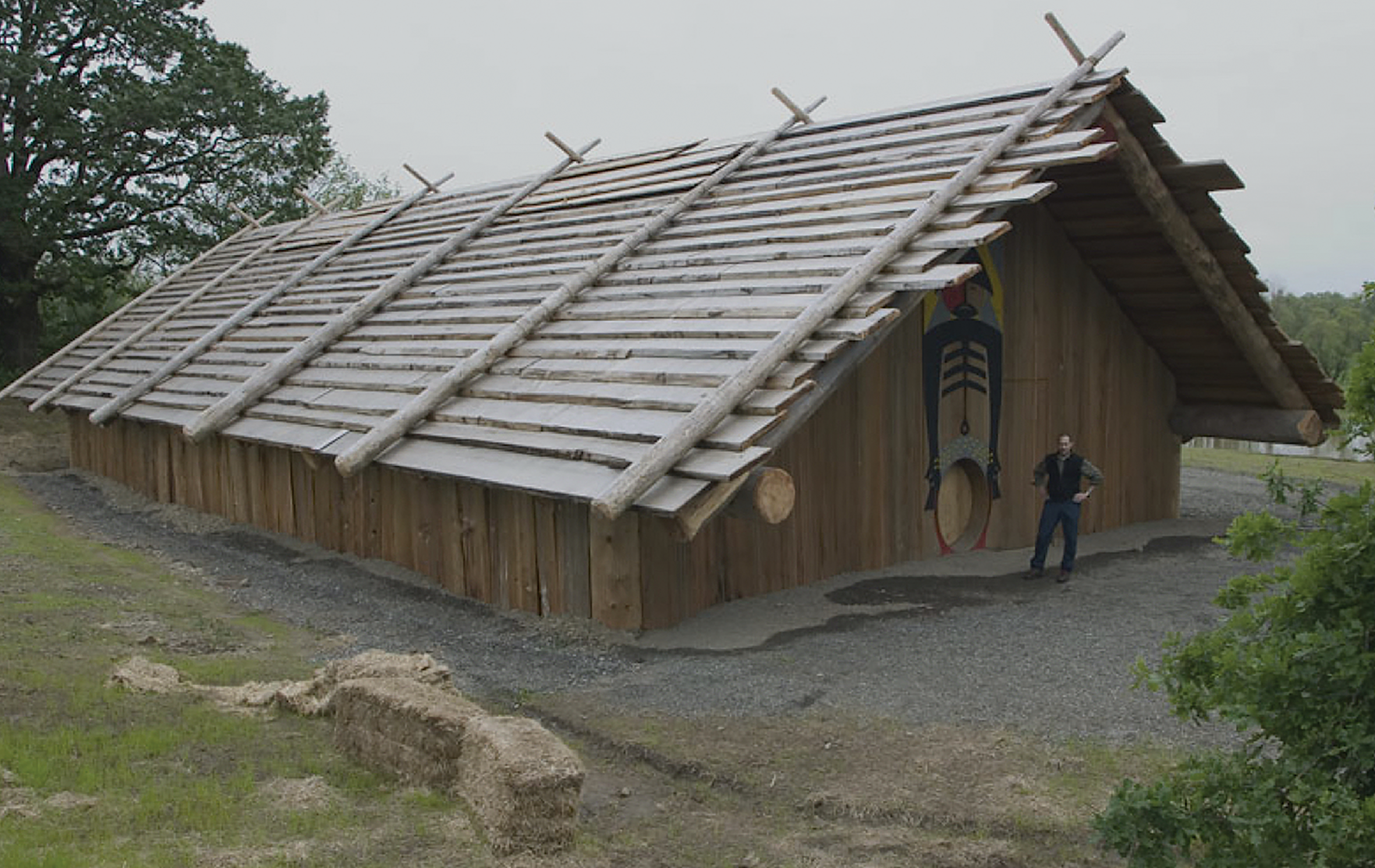
Figure 1. Reconstruction of a traditional Lower Columbia Valley plankhouse. Located near the Cathlapotle site, the architectural design draws on archaeological data from the Wapato Valley and Chinook tribal knowledge (photograph by K. Ames).
Other limitations of the data should be acknowledged. Households in Lower Columbia had individual histories covering as much as four centuries (Ames Reference Ames, Sobel, Gahr and Ames2006) and their fortunes in terms of wealth, income and demographics may have waxed and waned over time. Different formation processes and preservation conditions may have taken place within individual houses and across sites. While such variability cannot be entirely mitigated, the data are drawn from similar archaeological phenomena in similar environments, with comparable excavation and recovery techniques.
Using house area as a proxy for household status is well established in the Pacific Northwest (e.g. Coupland Reference Coupland1985; Hayden Reference Hayden1997; Archer Reference Archer and Cybulski2001; Grier Reference Grier, Christie and Sarro2006). This approach rests on broad ethnographic comparative studies (e.g. Netting Reference Netting1982) and ethnographic descriptions of some coastal regions where house size corresponds with household status and household wealth. This correspondence has been tested by examining labour and material costs for different sized post-and-beam houses and finding a strong correlation in the material, labour costs and house size (Ames Reference Ames, Coupland and Banning1996; Gahr Reference Gahr, Sobel, Gahr and Ames2006; Ames & Shepard Reference Ames and Shepard2019). While house size may reflect the number of people in a household, house sizes on the Pacific Northwest Coast also provide a reasonable, albeit imperfect, proxy for wealth differences.
Direct archaeological evidence for the storage capacity of a given house is rarely available. Historically, goods were kept in storage boxes and baskets stacked around the interior perimeters of houses, and/or suspended from racks under house roofs and outdoors (Hajda Reference Hajda1994). Storage capacity (i.e. house volume) can therefore be roughly estimated from ethnographically derived descriptions of floor area multiplied by house wall and roof heights (Ames Reference Ames, Coupland and Banning1996). As floor areas rather than wall heights typically remain visible in the archaeological record, this measure facilitates a useful approximation of storage capacity differences. Houses in the sample had subfloor storage facilities (Ames et al. Reference Ames, Smith and Bourdeaux2008), allowing storage capacity to be estimated independently of floor area, although we should bear in mind that such estimates underestimate storage capacity as they do not include the interior volume of the house structure.
The sample
The sample (Table 1) includes excavated houses from three sites along the Lower Columbia River, all dating to the last 500 years. Hajda (Reference Hajda1994) distinguishes permanent (winter) houses from seasonal (summer) houses. For our analysis, we selected only permanent houses from three sites: Clahclellah, Cathlapote and Meier (Figure 2).

Figure 2. The Lower Columbia River region and locations of sites discussed in the text (map by K. Ames).

Clahclellah
Clahclellah is located in the Columbia River Gorge and dates to c. AD 1700–1855 (Sobel Reference Sobel2017). The village was almost entirely excavated in the 1970s (Minor et al. Reference Minor, Toepel and Beckham1989; Sobel Reference Sobel2017). Its seven small houses (Table 1) were in two rows, and several houses were rebuilt at least once. The analysis uses the average floor area for houses with multiple floors. The seasonality of the village is a key issue: Minor et al. (Reference Minor, Toepel and Beckham1989) argue that it was a summer fishing village, while Sobel concludes that it was a more permanent village before the 1830s. We adopt Sobel's position based on observed house features, including the rows of storage pits flanking hearths set in boxes, which strongly resemble those seen in permanent houses in the Wapato Valley.
Cathlapotle
Cathlapotle was a large, permanent village in the Wapato Valley dating to c. AD 1350–1835 (Figure 3). A sample was excavated between 1991 and 1996 (Ames & Henry Reference Ames and Henry2017a–Reference Ames and Henrye; Ames & Brown Reference Ames and Brown2018). Six large structures (Table 1) were arranged in two rows paralleling a tributary of the Columbia River. The four largest structures were built by placing smaller structures end to end (Figure 3). This segmented construction is typical of the largest houses in the Wapato Valley, and is unique to it (Hajda Reference Hajda1994). Houses 1 and 4 were extensively excavated. House 1 had four segments, designated 1A, 1B, 1C and 1D from north–south. Segment 1A was not excavated. House 4 was unsegmented. All sampled houses had extensive subfloor storage pits or cellars and large central hearths.

Figure 3. Map of Cathlapotle showing modular house construction (map by E. Shepard).
The segmented houses pose a methodological problem: is each segment a separate house or household, or do the multiple segments form a single integrated household or ‘house’ in Levi-Straussian (Reference Levi-Strauss1983) terms (i.e. a social unit based on the house)? While the Cathlapotle project concludes that the combined segments represent ‘houses’ (e.g. Ames Reference Ames, Sobel, Gahr and Ames2006; Sobel Reference Sobel2017), each segment is sometimes treated separately for analytical and comparative purposes. Here, Gini coefficients are calculated for both the individual segments and the larger, multi-segment structures.
Meier
Meier is also in the Wapato Valley and, as far as is known, contains only a single large, unsegmented house (Table 1). The site was established in c. AD 1000, and the excavated house dates to c. AD 1400–1810 (Ames & Brown Reference Ames and Brown2018). It was a substantial structure (Ames & Shepard Reference Ames and Shepard2019), with massive subfloor storage features (Ames et al. Reference Ames, Smith and Bourdeaux2008) flanking a row of central hearths. The house was clearly intended for permanent habitation. For analytical purposes, we divide it into thirds, labelled north, central and south, corresponding to hearth groups defined by the arrangement of internal structural features encountered during excavation. These divisions are analytically analogous to house segments at Cathlapotle.
Methods
Gini coefficients were calculated using the Gini coefficient module in StatsDirect@ v.3.1.20, which controls for small sample sizes by calculating an unbiased estimate of the population Gini coefficient. StatsDirect also calculates 0.95 confidence intervals for the Gini coefficient using bootstrapping with 100 000 iterations. Confidence intervals are recommended by Peterson and Drennan (Reference Peterson, Drennan, Kohler and Smith2018) to improve comparability, and by Prentiss et al. (Reference Prentiss, Foor, Murphy, Kohler and Smith2018b) to control for small sample sizes. Multiple coefficients were calculated based on floor area and storage capacity for different iterations of the sample (Table 2).
Table 2. Samples analysed.

Floor areas are as given in the reports cited. Storage capacity is the estimated volumes of storage pits based on reported pit dimensions, using the formula for the volume of a cylinder: V = πr 2h, where r is the radius and h is the height, or depth. For Meier and Cathlapotle, total pit volume was calculated by:
1) Counting the pits in the excavated area of the house.
2) Calculating the number of pits/m2/sampled area.
3) Estimating the total number of pits in the house by multiplying excavated pits/m2/sampled area by total house area.
4) Calculating the mean pit volume in litres for sampled pits.
5) Multiplying that figure by the estimated total number of pits for the house.
As the Clahclallah houses were completely excavated, it was not necessary to estimate the number of pits per house. Most houses, however, were rebuilt two or three times with varying numbers of pits. The mean number of pits was therefore used, as was the mean floor area.
The hypothesis that storage capacity potentially reflects anticipated household income is assessed by examining the density of faunal remains (number of identified specimens, NISP/m3) in the various house segments. This assumes that income was related to subsistence and is represented, at least in a relative sense, by densities of faunal remains as a crude estimate of the abundance of one form of food and in the absence of evidence for other perishable foodstuffs. Data are limited to the excavated houses and house segments at Cathlapotle and Meier, as the faunal remains recovered at Clahclellah are unreported. The relationship is evaluated using linear regression, with storage capacity as the independent variable and faunal NISP/m3 as the dependent variable.
Results
Gini coefficients and 0.95 confidence intervals are presented in Table 3 and Lorenz curves in Figure 4. Figure 5 shows the Gini coefficients and confidence intervals.

Figure 4. Lorenz curves for house floors and storage capacities (figure by C. Grier).

Figure 5. Gini coefficients and confidence intervals (figure by K. Ames).
Table 3. Gini coefficients.

Floor area
Floor-area analysis suggests no wealth inequality at Clahclellah. At Cathlapotle and in the Wapato Valley, wealth differences are weakly expressed in the three samples based on house segments. By contrast, they are strongly expressed in the three samples based on complete houses.
Storage
The Gini coefficients for storage capacity are consistently higher than those for floor area, mirroring the pattern observed by Kohler and Higgins (Reference Kohler and Higgins2016) and Bogaard et al. (Reference Bogaard, Styring, Whitlam, Fochesato, Bowles, Kohler and Smith2018) (Table 3).
Income
There is a strong relationship between faunal NISP/m3 and storage capacity in this limited sample. The linear regression yielded an adjusted R2 of 0.89 (Table 4).
Table 4. Linear regression* of storage capacity in litres against faunal number of identified specimens (NISP)/m3 for faunal remains retrieved using a 6.4mm mesh.

* Model: Total NISP/m3 = −2.412 + (1.069) storage, [F(1,6) = 20.8, p = 0.006. R2 = 0.81].
Discussion
Floor area
The floor-area results depend on whether the house segments represent separate houses or parts of larger ‘houses’. In the former, the coefficients fall within the Kohler et al. ranges for foragers (Kohler et al. Reference Kohler2017: fig. 2, Reference Kohler, Kohler and Smith2018: fig. 11.2), although their sample in the former study includes only five forager examples, and in the latter only three. By contrast, the ‘house’ results show strong wealth differentiation, with a mean Gini coefficient of 0.35, well above the middle range for horticulturalists in the Kohler et al. samples and in the upper portion of that range for the agriculturalists (Kohler et al. Reference Kohler2017: fig 2, Reference Kohler, Kohler and Smith2018: fig. 11.2). As we consider the segments to form parts of larger ‘houses’, the Gini coefficient based on the Cathlapotle houses—not the house segments—offers the more accurate reflection of wealth differentials in the village, and the Wapato Valley more generally. The differences in the Gini coefficients between the two iterations of these samples, however, illustrates the importance of deciding what constitutes a house in this kind of analysis.
How do these results shed light on inequality at Clahclellah? Was it an egalitarian village? Although it has the lowest Gini coefficients among the three villages, Sobel (Reference Sobel2017) found evidence for different strategies of establishing prestige among the Clahclellah houses. Furthermore, in at least one region of the Northwest Coast—Prince Rupert Harbour in northern British Columbia—villages exhibiting little differentiation in house size were inhabited at the same time as villages with marked differences in house size (Martindale et al. Reference Martindale, Letham, Supernant, Brown, Edinborough, Duelks and Ames2017), before c. 1500 cal BP. This illustrates the likelihood of village-level variation in household wealth, or in the manner of displaying wealth within a region. This issue is probably not limited to the Pacific Northwest Coast.
Storage
The storage-based Gini coefficients are consistently higher than the floor-area coefficients, irrespective of how the samples are organised. The coefficients vary in the strength at which differential wealth or income is expressed: weakly at Clahclellah, stronger for the Wapato Valley and quite strong for the full sample. By replicating the findings of other studies where this pattern was observed (Kohler & Higgins Reference Kohler and Higgins2016; Bogaard et al. Reference Bogaard, Styring, Whitlam, Fochesato, Bowles, Kohler and Smith2018), our results cross-cut geography, subsistence economy and time, suggesting that the pattern is indeed strong. What it represents is another question. It is possible that house-floor area reflects other elements such as household size, or that it is more constrained in its magnitude of variation than storage capacity.
Income
The assessment of the relationship between income, as measured by faunal NISP/m3, and storage capacity is limited to the three excavated Cathlapotle house 1 segments, Cathlapotle house 4 and the three units of the Meier house divided into thirds. Despite the small sample, there is a strong positive linear relationship between storage capacity and the density of faunal remains. The regression, however, masks differences in the scale of storage and production across the sample. These differences can be probed by comparing the storage capacity by floor area (Table 1) and the densities of the faunal remains. This shows that the relationships between floor area, storage capacity and income are not straightforward.
Although the notion of ‘income’ may be a useful simplifying concept to decipher the difference between material wealth and storage in large-scale comparative analyses, for this small-scale study, it is an oversimplification. At this scale, ‘income’ encompasses household socioeconomic strategies built around storage and surplus (Ames Reference Ames, Sobel, Gahr and Ames2006). Storage capacity per floor area provides a window into these strategies. On the reasonable assumption that floor area correlates broadly with household population (e.g. Narroll Reference Narroll1962), litres of storage per floor area serves as a proxy for litres of storage per capita. Thus, it measures surplus production following De Lucia and Morehart's (Reference De Lucia, Morehart, Morehart and De Lucia2015: 74) definition of surplus as “a strategy to meet overlapping institutional and social needs”.
A broader consideration of the houses suggests that the sample forms a continuum of production intensity from Clahclellah houses (low) to Meier (high). This continuum reflects interpreted differences in production strategies related to establishing and maintaining household prestige (Ames & Gardner-O'Kearny Reference Ames, Gardner-O'Kearny, Ames and Henry2017; Sobel Reference Sobel2017). Meier was a very high production household, as indicated by its overall storage capacity, density of faunal remains and litres of storage by floor area. These aspects are all high compared to the other houses in the sample, and seem high for the house population (Table 1), suggesting significant surplus production. The Meier house was also characterised by a relatively complex division of labour (Smith Reference Smith2015; Ames & Gardner-O'Kearny Reference Ames, Gardner-O'Kearny, Ames and Henry2017).
The overall production at Cathlapotle house 1 is less intense than at Meier, although it approaches Meier levels in house 1C, despite its intermediate storage in litres/m2; house 1B is a low-production house segment. House 1D has the highest storage capacity but has intermediate densities of faunal remains. House 1 also had a very complex division of labour spanning all excavated house segments, of which house 1C was the industrial heart (Smith Reference Smith2015; Sobel Reference Sobel2017), with significant craft production. Less production is evident in house 1D. Although segmented, house 1 was probably a ‘house’ in the Levi-Straussian (Reference Levi-Strauss1983) sense, and hence these segments reflect an integrated household economy. Despite a relatively high storage in litres/m2, house 4 has rather low production levels, as measured by faunal remains densities, and a somewhat simpler division of labour (Smith Reference Smith2015). Sobel (Reference Sobel2017) concludes that production levels in the Clahclellah houses were generally low to average. While they most resemble houses 1B and 4 at Cathlapotle in floor area, their storage litres/m2 are most similar (although smaller overall) to those of house 1B. This again indicates low levels of production. Unfortunately, no faunal data are available for Clahclellah.
Combined with other evidence (Ames & Gardner-O'Kearny Reference Ames, Gardner-O'Kearny, Ames and Henry2017), our results for the Meier household suggest that its economy was geared towards producing large surpluses of processed food that was used to maintain or expand the household's prestige. Cathlapotle house 1 had a more mixed strategy, which involved both surpluses in processed food and exchange of raw materials and finished goods. The strategy of Cathlapotle house 4 is less clear. Sobel argues that households in Clahclellah had different prestige-enhancing strategies, one of which depended on relational and embodied wealth (not Sobel's terms) and another on craft production. Neither, however, required significant surplus food production.
Conclusions
This study replicates, for the Pacific Northwest Coast, the previously observed pattern of storage capacity yielding higher Gini coefficients than floor area as a proxy for wealth. While only a few studies have documented this pattern, they cross-cut time, space and subsistence mode. In this study, the pattern holds regardless of how the sample is organised. Combined, this evidence points to a significant relationship between wealth (as measured by floor area) and storage capacity in the archaeological study of the origins and development of social and economic inequality. Kohler and Higgins (Reference Kohler and Higgins2016) and Bogaard et al. (Reference Bogaard, Styring, Whitlam, Fochesato, Bowles, Kohler and Smith2018) consider storage capacity as a proxy measure for anticipated income. Here then, it can be viewed as reflecting surplus, and taken to mean that variation in the Gini coefficient reflects both the surplus and surplus-deploying strategies. Such a surplus is considered here to be an anticipated surplus. In other studies (e.g. Puleston et al. Reference Puleston, Tuljapurkar and Winterhalder2014; Winterhalder et al. Reference Winderhalder, Puleston and Ross2015), it has been attributed to provisioning for potential food shortages or increases in the number of people to be fed (e.g. Prentiss et al. Reference Prentiss, Foor, Cross, Harris and Wanzenried2012). This study also illustrates problems with the archaeological application of Gini coefficients discussed by others, including sample size and the definition of houses (e.g. Betzenhauser Reference Betzenhauser, Kohler and Smith2018), and demonstrates the importance of calculating the coefficient on several iterations of the sample.
Finally, our study demonstrates the usefulness of the Gini coefficient as a method for investigating inequality through deep time. Increasing the number of case studies of sedentary fisher-hunter-gatherers will be critical, as they represent an important context in which significant social inequalities emerged in small-scale, non-agricultural human societies (Ames Reference Ames, Price and Feinman2010; Grier Reference Grier, Finlayson and Warren2017). Our results indicate that non-agricultural societies can embody levels of inequality equal to or greater than other, similarly scaled agricultural societies. The specific strategies used for mobilising wealth and surplus to construct enduring inequalities may be effectively revealed by contrasting Gini coefficients derived from different proxies. These may trace different aspects of wealth deployment in the construction of social inequalities from more egalitarian social practices.
Acknowledgements
The excavations, analyses and reporting for Meier and Cathlapotle were funded by Portland State University, Ray and Jan Auel, U.S. Fish and Wildlife Service, the National Science Foundation, and the National Endowment for the Humanities. Our thanks to the Confederated Tribes of Grand Ronde for their support of the Meier Project, and the Chinook Indian Nation for their support of the Cathlapotle Project. This article was initially submitted by the first author, Ken Ames. During its peer review, Ken fell ill and passed away. This study is mainly his work. Colin Grier edited the manuscript based on reviewer comments, allowing it to be published in its final form. The archaeological community will dearly miss Ken and his contributions to our discipline and collective understanding of the past.


