


1. INTRODUCTION
1.1. Motivation for aircraft trajectory prediction
The rising demand for air travel has led to increasingly congested skies in some of the busiest regions of the world, e.g. Europe and North America. With this growth predicted to continue, there is an urgent need to address the capacity constraints in both the terminal areas and en-route airspace. In the en-route region, airspace capacity is limited by the workload of Air Traffic Controllers (ATCos) and a crucial component of this workload is that required to detect and resolve conflicts (Majumdar and Ochieng, Reference Majumdar and Ochieng2002). As a result, a variety of automated Decision Support Tools (DSTs), both ground-based and airborne, are continuously being designed and improved to assist controllers, thus reducing their workload. At the heart of such efforts lie time-based traffic management tools (useful for trajectory optimisation purposes), and Conflict Detection and Resolution (CDR) tools that allow for a higher number of user-preferred flight paths.
The central component of many DSTs is the ability to model and predict aircraft trajectories, i.e. Trajectory Prediction (TP). In the future Communications Navigation Surveillance/Air Traffic Management (CNS/ATM), DSTs should be able to provide conflict-free trajectories with their associated error margins (EUROCONTROL, 1998). Specifically, with the aid of on-board and satellite navigation and communications technologies, each aircraft will be able to predict its own trajectory and to use the information to negotiate and re-negotiate, in real time, a four-dimensional (4D) Flight Plan (FP) with surrounding aircraft. This should, in theory, provide airborne autonomous separation and give conflict-free tracks between departure and destination airports in the form of 4D profiles to be accurately adhered to by aircraft. Using this capability, surveillance methods such as Automatic Dependent Surveillance-Broadcast (ADS-B), Traffic Information System (TIS) and Airborne Separation Assurance System (ASAS), which is a tool that devolves responsibility for safe separation to the pilot (Casaux and Hasquenhoph, Reference Casaux and Hasquenhoph1997), should provide additional safety measures required to operate in a more flexible airspace. Because of the potential benefits, 4D navigation and trajectory prediction capabilities are core elements of the Single European Sky ATM Research (SESAR) programme for the modernisation of the European ATM system (EUROCONTROL, 2007b).
These systems will also have profound impacts on ATM functions and working methods of pilots and ATCos. In the “Free-Flight” (FF) concept, for example, the greatest degree of autonomous operations has been proposed, with pilots being free to choose their preferred route between departure and destination airports. The FF concept envisages each aircraft communicating with both ground controllers and proximate aircraft to negotiate and establish conflict free flight paths. Most of the FP negotiation will be carried out through automated communications and digital data links to supplement radio-based voice communications. In line with the USA, the promotion of FF is also defined as one of the aims of the EUROCONTROL ATM 2000+ programme (EUROCONTROL, 1998). Although this will occur gradually, with increasing autonomous operations, the decision making responsibility will progressively shift towards the crew, thereby minimising ATCos' workload and increasing airspace capacity.
Modern aircraft are technologically advanced and have on board complex systems such as Flight Management Computers (FMCs) and satellite navigation systems (Honeywell, 1989). Whilst airborne Flight Management Systems (FMSs) have been developed to provide cost-efficient flight guidance for individual airplane operations, crew need further assistance and more sophisticated DSTs to let them manage their own trajectory, and to ensure separation with the surrounding traffic. In particular, accurate TP models are required for the DSTs involved in the implementation of CDR schemes (Kuchar and Yang, Reference Kuchar and Yang2000). Examples here include the Interim Future Area Control Tools Support (iFACTS) and En-route Air Traffic Organiser (ERATO) tools envisaged for Europe (EUROCONTROL, 2007a).
1.2. Trajectory prediction models available in the open literature
Current approaches for TP make a number of assumptions in order to simplify the mathematical models of aircraft motion. This, in turn, has an impact on the prediction accuracy and then on the Conflict Resolution (CR) strategies which can subsequently be employed (Kuchar and Yang, Reference Kuchar and Yang2000).
The TP model proposed in the framework of the HYBRIDGE Project (Glover and Lygeros, Reference Glover and Lygeros2003 and Reference Glover and Lygeros2004) adequately simulates aircraft behaviour from the point of view of an ATCo, while maintaining a workable degree of simplicity. The aircraft dynamics are modelled through a six-Degrees of Freedom (DOF) Point Mass Model (PMM), while typical values for aircraft performance parameters are obtained from the EUROCONTROL Base of Aircraft Data (BADA) database (EUROCONTROL, 2004). The basic input to the TP algorithm is a FP consisting of a sequence of Waypoints (WPs), each one temporally referenced with an Expected Time of Arrival (ETA). Finally, the aircraft speed when flying between two WPs is determined based on the speed profiles provided by BADA and not based on ETA requirements.
Similar to the scheme proposed in the HYBRIDGE Project, several other TP methods do not consider information about ETA at the most important points of the intended aircraft route. These methods are usually referred to as Three-Dimensional (3D) TP Models. However, such an uncertainty may lead to significant inaccuracies, especially if the prediction is performed over an extended time-horizon. As a result, a number of TP methods, referred to as 4D TP Models, that take into account ETA and related data, have been proposed. An example of such models is by Slattery and Zhao (Reference Slattery and Zhao1997), where the trajectory synthesis algorithms used in the Center-TRACON (Terminal Radar Approach Control) Automation System (CTAS) are presented. In the process proposed in Slattery and Zhao (Reference Slattery and Zhao1997), both the horizontal and vertical trajectories are divided into a series of flight segments, which can be assumed to be flown by pilots by holding constant variables. Flight speeds related to such segments are then iterated to meet ETA requirements (Slattery and Zhao, Reference Slattery and Zhao1997). As significant computational effort may be required for the iteration process, such a TP synthesis scheme may not be suitable for airborne implementation, as computational resources available on the aircraft cockpit are limited. Alternatively, 4D TP models can be derived from 3D TP algorithms by adding a process for assigning either different speeds (depending on the ETAs) or different climb or descent profiles (Glover and Lygeros, Reference Glover and Lygeros2004).
1.3. Overview of the proposed model
This paper builds on the methods used by the HYBRIDGE Project to develop an enhanced 4D TP model. Aircraft performance parameters are obtained from the EUROCONTROL BADA dataset, augmented with additional parameters to improve prediction accuracy. Aircraft dynamics are modelled through the six-DOF PMM used in the HYBRIDGE Project, and a set of variables identifying the aircraft state is defined on the basis of the PMM equations. Aircraft motion also accounts for the effects of the wind, with the wind-field determined from accurate wind activity forecasts and/or measurements.
An essential input to the proposed TP process is a sequence of Trajectory Change Points (TCPs), which are defined as those points where a significant change in the aircraft state is required. Each TCP is temporally referenced with its corresponding ETA and includes additional information on aircraft operating modes. Any modification in aircraft state (e.g. height, heading, or speed) can be modelled using TCPs. The sequence of TCPs forms a Flight Script (FS), which can be updated during flight, for example to take into account unexpected advisories from ATCos. Such a script is shown to effectively describe the aircraft intent, which is the set of instructions defining without any ambiguity how an aircraft is to be operated within a given timeframe (Vilaplana, Reference Vilaplana Ruiz2005).
When flying between two TCPs, aircraft speed is estimated on the basis of both the actual aircraft position and the ETA related to the subsequent TCP. Constraints due to aircraft performance are also considered. The proposed scheme is then four dimensional providing a more accurate definition of the speed profiles than those provided by the BADA database, where the information relevant to the ETAs is not considered.
Finally, a new method to model the aircraft lateral guidance control system is proposed. While in the system used in Glover and Lygeros (Reference Glover and Lygeros2003 and Reference Glover and Lygeros2004) the Heading Error (HE) and the Cross Track Error (CTE) from the reference path are controlled separately, in the method proposed in this paper the effects of the CTE are incorporated in the HE. Such an approach emulates practical pilot procedures and allows both the CTE and the HE to be adjusted very quickly, taking into account limitations due to aircraft performance and passenger comfort.
1.4. Paper structure
A high level architecture of the proposed TP model is outlined first, followed by a discussion of input data, together with the approach used for aircraft intent modelling. A detailed description of the model is then presented, including additional operating parameters for representing aircraft performance. Particular attention is also given to the schemes used for aircraft speed settings and for lateral guidance control system modelling. A subsequent section describes the approach taken to validate the TP algorithm. Finally, a summary of the main contributions of the paper is presented.
2. HIGH LEVEL ARCHITECTURE OF THE PROPOSED TRAJECTORY PREDICTION MODEL
The high level architecture of the proposed TP model is presented in Figure 1. The computation process is carried out within what is commonly referred to as a Trajectory Engine (TE) block, where two systems continuously interact over time. The first is a Non-Linear (NL) control system which captures aircraft dynamics and is characterised by six state variables, four inputs and three disturbances. As three of the six state variables are represented by aircraft coordinates, the evolution of the state over time provides the trajectory prediction. The values of the input variables are decided by the second system, which models the aircraft FMS. Such a block is a controller which, throughout the trajectory computation process, measures the state of the aircraft dynamics and uses it in conjunction with aircraft intent information, captured in a Flight Script (FS), to determine the values of the input variables.
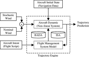
Figure 1. Basic framework for the proposed trajectory prediction model.
Aircraft performance parameters have an impact on both aircraft dynamics and FMS models. As a consequence, the EUROCONTROL BADA dataset is required as an underlying model for the proposed TE. A further underlying model deals with atmospheric conditions and is given by the International Standard Atmosphere (ISA) provided by the International Civil Aviation Organisation (ICAO) (ICAO, 1964).
In addition to the FS, which feeds the FMS model, other inputs are needed by the TE to support the integration of the set of equations that describe aircraft dynamics. Firstly, the aircraft initial state must be specified using navigational data or airborne instrumentation. Secondly, as the three disturbance variables are given by the three components of the wind speed, an accurate wind-field must be set up. Following the same approach suggested in the HYBRIDGE project, the wind-field is evaluated, in this paper, as the sum of two components, nominal and stochastic. The former is derived from wind activity forecasts and/or measurements, and the latter accounts for both wind uncertainties and spatial correlation properties. It should be noted that further sources of uncertainty are assumed with respect to the FS, information relevant to aircraft initial state, and aircraft performance parameters.
According to the proposed approach, the TP problem is closely related to that of an autopilot design problem. For example, assume that, at a certain time, a turn, fly-over or fly-by, is required by the FS. This happens every time the aircraft must change its heading to move toward the next WP. As in an autopilot system, a new set of input variables is then automatically decided by the FMS block, taking into account the actual aircraft state. Finally, the aircraft dynamics block is used to evaluate the effects of these new inputs on the aircraft state, thus updating the predicted trajectory.
The functional elements of the high level architecture in Figure 1 are detailed in subsequent sections, starting with the input data, followed by a comprehensive description of the Aircraft Dynamics System, the FMS Model and their interactions.
3. INPUT DATA
3.1. Aircraft intent (flight script)
Aircraft intent is defined as a structured set of instructions identifying without any ambiguity how an aircraft is to be operated within a timeframe (Vilaplana, Reference Vilaplana Ruiz2005). A valid instance of aircraft intent is formed by a time-ordered sequence of non-overlapping operations. An operation is defined as a set of compatible instructions that unambiguously determines aircraft motion during a time interval referred to as an operation interval. In the proposed TP model, the trajectory computation process is performed by the TE and is based on the integration of a set of equations describing aircraft motion. Consequently, every aircraft intent instruction must have a mathematical formulation which is compatible with the equations of motion used by the TE (Vilaplana Ruiz, Reference Vilaplana Ruiz2005).
In the proposed method, aircraft intent is modelled using a FS which is an ordered sequence of TCPs. TCPs are defined as the points where a significant change in the aircraft state is required. Such a state includes any information useful for aircraft behaviour characterisation, such as horizontal position, height, speed, Rate of Climb or Descent (ROCD), or heading angle. Particular operating modes, such as flap setting or spoiler configuration for expedited descent, are also considered for an accurate and reliable state identification.
The data related to each TCP are organised in appropriate fields. The following minimal specifications are mandatory for all TCPs: (a) horizontal position (latitude and longitude), (b) height Above Sea Level (ASL) or above some other reference, (c) ETA measured from a specified event, e.g. aircraft Take-Off (TO), (d) Turn Mode (TM), fly-over or fly-by, (e) Holding Mode (HM), which indicates if the TCP belongs, or not, to a holding area and (f) Expedited Descent Mode (EDM), which specifies the spoiler configuration adopted by an aircraft until the next TCP is reached. The flags TM, HM and EDM refer to particular aircraft operating modes and their specifications are intended to be set for the next segment upon reaching the TCP. Further operating modes and/or aircraft configurations can be considered using additional flags.
TCPs are ordered according to increasing values of the ETAs in the FS and can be shown to effectively model aircraft intent. In fact, each TCP identifies the following instructions, whose parameters are directly specified by the TCP's fields, (a)–(f), listed above:
1. The aircraft must be at the specified point, {TCP fields (a) and (b)}, at the specified time, {TCP field (c)}.
2. A TM of the specified type, {TCP field (d)}, is required at the TCP.
3. If necessary, i.e. according to {TCP field (e)}, apply aircraft configuration settings for HM as soon as the TCP is reached.
4. If necessary, i.e. according to {TCP field (f)}, apply aircraft configuration settings for EDM as soon as the TCP is reached.
Assuming that the FS contains N TCPs, the instructions, 1 to 4 (above), related to a given TCP, i (i=1, …, N), are compatible and simultaneously active during the same execution interval, ΔT i=[t i−1 t i], where t i−1 and t i are the times when the aircraft reaches the TCPs i−1 and i respectively (in general, such times may be different from the corresponding ETAs). The integration of the equations of motion used in the proposed TP model, in conjunction with the mathematical conditions imposed by the instructions 1 to 4, results in a unique trajectory for the execution interval. In summary, the instructions 1 to 4 are compatible, simultaneously active and able to unambiguously determine the aircraft motion during their execution interval. Therefore, they give rise to an operation whose operation interval exactly matches the execution interval. These arguments can be repeated for all the TCPs of the FS. Furthermore, the trajectories computed without any ambiguity in each operational interval can be merged together to form a unique, continuous, predicted trajectory.
Given the above, it can be seen that the instructions associated with the TCPs give rise to a time-ordered sequence of non-overlapping operations, each one with an associated operational interval. As a result, these instructions form a valid instance of aircraft intent (Vilaplana Ruiz, Reference Vilaplana Ruiz2005), which can be modelled efficiently by the proposed FS.
A number of heterogeneous input data types can be summarised in the suggested FS. Intended routes, airlines' preferences, standard operational procedures and ATCo constraints can be suitably modelled using TCPs. Adaptation data can also be considered. Hazard Zones, No-fly Zones, or regions with severe weather conditions can be avoided by introducing suitable TCPs. Finally, during flight, the FS can be updated in real time, by adding or modifying TCPs. Therefore, even unexpected advisories from ATCos can be considered and the effectiveness of airborne CR strategies can be verified promptly.
3.2. Nominal and stochastic wind-field
The effect of wind on aircraft motion is accounted for by using the same approach as outlined in the HYBRIGDE Project. The wind-field is evaluated as the sum of two components, nominal and stochastic. The nominal wind is modelled as a look-up table, similar in temporal and spatial resolution to the meteorological data available to ATCos, with appropriate interpolation algorithms. Wind samples are generally available from measurements or weather forecast. Deviations from the nominal wind can be accounted for in the stochastic wind component (assumed to be zero in the current implementation of the TP model), which is a random field with an assigned statistical structure. For example, in the HYBRIDGE Project, the stochastic component is assumed to be jointly Gaussian with a known correlation function. Work is in progress to design a model for the stochastic wind component which is both accurate and computationally efficient.
3.3. Aircraft initial state
In order to integrate the set of the equations describing aircraft dynamics, the TE requires data on the aircraft initial state (i.e. the state at the start of the TP process). Aircraft initial position and speed can be obtained from navigation data. Further information, such as aircraft initial attitude, flap setting, or spoiler configuration, can be derived from airborne instrumentation.
4. AIRCRAFT DYNAMICS
From the point of view of an ATCo, an aircraft can be adequately modelled using a six-DOF PMM, which can be easily derived from basic aerodynamics. Furthermore, additional simplifications can be made when dealing with civil aircraft. For example, it is possible to assume that aircraft operate near trimmed flight conditions all the time, so the angle of attack can be reasonably assumed to be zero. As shown in the HYBRIDGE Project, aircraft motion can then be captured by a non-linear (NL) control system with six state variables, three inputs and three disturbances. Such a system is discussed in the following subsections.
4.1. State variables, inputs and disturbances
Three of the six state variables are aircraft horizontal position, x and y, and aircraft altitude ASL, h. The evolution of such variables over time provides aircraft trajectory, with the assumption that the Earth can be locally approximated as a non-rotating flat surface throughout the TP process. The remaining state variables are True Air Speed (TAS), V, heading angle, ψ, and aircraft mass, m. TAS is defined as the actual speed of aircraft relative to the surrounding air. In the proposed model, the heading angle is defined as the angle formed between the positive x axis (east direction) and the direction of the projection of the TAS vector onto the horizontal plane, (x, y). Such an angle is measured positively counter clockwise (CCW) from the east direction. An additional state is introduced to keep track of changes in the aircraft mass. Because of fuel consumption, such changes can be significant, especially over longer flights. In summary, a state vector can then be introduced as: ![]() .
.
In the HYBRIDGE Project, the engine thrust, T, the bank angle, φ, and the flight path angle, γ, are considered as input variables for the NL system. Such variables emulate practical control inputs available to the pilot. As a consequence of the assumed trimmed flight conditions, the engine thrust is supposed to always act parallel to the TAS vector. Furthermore, the pilot controls several aircraft configuration aspects, such as spoilers, leading edge slats, trailing edge flaps or landing gear settings. Such features have a significant impact on the drag coefficient, C D. For this reason, in this work, such a coefficient is considered as an additional input to the system. An input vector is then introduced as ![]() .
.
Finally, the three disturbances are given by the wind-field, which is modelled through its speed. An available function, W: IR 3→IR 3, provides the three components of the wind speed vector related to each point belonging to the space of interest, ![]() . As a consequence, a disturbance vector can be introduced as
. As a consequence, a disturbance vector can be introduced as ![]() .
.
4.2. The non-linear control system
Once the vectors relevant to state variables, inputs and disturbances are defined, aircraft motion can be shown to be captured by the following NL control system (Glover and Lygeros, Reference Glover and Lygeros2003 and Reference Glover and Lygeros2004):
![{\dot{x}} \equals \left[ {\matrix{ {\dot{x}_{\setnum{1}} } \hfill \cr {\dot{x}_{\setnum{2}} } \hfill \cr {\dot{x}_{\setnum{3}} } \hfill \cr {\dot{x}_{\setnum{4}} } \hfill \cr {\dot{x}_{\setnum{5}} } \hfill \cr {\dot{x}_{\setnum{6}} } \hfill \cr} } \right] \equals \left[ {\matrix{ {x_{\setnum{4}} \cos \left( {x_{\setnum{5}} } \right)\cos \left( {u_{\setnum{3}} } \right) \plus w_{\setnum{1}} } \hfill \cr {x_{\setnum{4}} \sin \left( {x_{\setnum{5}} } \right)\cos \left( {u_{\setnum{3}} } \right) \plus w_{\setnum{2}} } \hfill \cr {x_{\setnum{4}} \sin \left( {u_{\setnum{3}} } \right) \plus w_{\setnum{3}} } \hfill \cr { \minus \left[ {\left( {{{u_{\setnum{4}} S\rho } \mathord{\left/ {\vphantom {{u_{\setnum{4}} S\rho } 2}} \right. \kern-\nulldelimiterspace} 2}} \right) \cdot \left( {{{x_{\setnum{4}}^{\setnum{2}} } \mathord{\left/ {\vphantom {{x_{\setnum{4}}^{\setnum{2}} } {x_{\setnum{6}} }}} \right. \kern-\nulldelimiterspace} {x_{\setnum{6}} }}} \right)} \right] \minus \left[ {g\sin \left( {u_{\setnum{3}} } \right)} \right] \plus \left( {{{u_{\setnum{1}} } \mathord{\left/ {\vphantom {{u_{\setnum{1}} } {x_{\setnum{6}} }}} \right. \kern-\nulldelimiterspace} {x_{\setnum{6}} }}} \right)} \hfill \cr {\left[ {\left( {{{C_{L} S\rho } \mathord{\left/ {\vphantom {{C_{L} S\rho } 2}} \right. \kern-\nulldelimiterspace} 2}} \right) \cdot \left( {{{x_{\setnum{4}} } \mathord{\left/ {\vphantom {{x_{\setnum{4}} } {x_{\setnum{6}} }}} \right. \kern-\nulldelimiterspace} {x_{\setnum{6}} }}} \right)} \right] \cdot \sin \left( {u_{\setnum{2}} } \right)} \hfill \cr { \minus \eta \cdot u_{\setnum{1}} } \hfill \cr} } \right] \equals f\left( {{\bf x}\comma {\bf u}\comma {\bf w}} \right)](https://static.cambridge.org/binary/version/id/urn:cambridge.org:id:binary:20151022093911885-0970:S0373463308004761_eqn1.gif?pub-status=live)
In the system (1), S is the aircraft total wing surface area, ρ is the air density and g is the acceleration due to gravity (9·81 ms −2). Furthermore, C L indicates the aerodynamic lift coefficient and η is a factor related to fuel consumption. The wing surface area and the fuel consumption factor can be obtained from the BADA Database, while the air density is determined according to the International Standard Atmosphere (ISA) model. Since the model reflects trimmed flight conditions for the aircraft, the lift coefficient is set to ensure that the vertical component of the lift balances the weight of the aircraft, including a correction term for changes in the bank angle, i.e. C L=[2x 6g]/[ρ · x 42Scos(u 2)].
The state and the input variables of the system (1) are subject to the following constraints: maximum height, minimum and maximum TAS, minimum and maximum mass, maximum engine thrust, minimum and maximum bank angles, and minimum and maximum flight path angles. For a specific aircraft, the values of such bounds can be derived from the BADA database.
It should be noted that neither the effects of the vertical wind gradient, nor the rate of change of the wind velocity, are taken into account in the proposed NL system (1). However, the system is generally a good approximation assuming that wind speed does not change quickly in time or space (Glover and Lygeros, Reference Glover and Lygeros2003).
The NL system in (1) is equivalent to what is referred to in the BADA documentation as a Total Energy Model (TEM). Such a model effectively equates the rate of work done by the forces acting on the aircraft to the rate of change in its total (potential plus kinetic) energy. The forces acting on the aircraft, under the assumptions imposed so far, are shown in Figure 2, where L=[(C LSρ/2) · x 42] and D=[(u 4Sρ/2) · x 42] denote the lift and drag forces, respectively (Glover and Lygeros, Reference Glover and Lygeros2004).

Figure 2. Forces acting on the aircraft under the assumption of trimmed flight conditions.
According to the TEM, it has been shown in EUROCONTROL (1987) that the ROCD, ![]() , can also be expressed as:
, can also be expressed as:
where the term f(M) is an Energy Share Factor (ESF) which is a function of the Mach number, M. While following a selected speed profile during climb or descent, such a factor determines the ratio of the available power which is allocated to climbing/descending (increasing/decreasing potential energy) to accelerating/decelerating (increasing/decreasing kinetic energy) EUROCONTROL (1987).
The ESF is used extensively in the BADA documentation and also in airline procedures. Furthermore, it is related to the flight path angle through the following relationship:
Such an equation is obtained through the comparison of the two expressions for the ROCD, (1) and (2), with the assumption, normally verified, that the vertical wind component is negligible. For a given thrust setting, equation (3) relates each value of the ESF to a unique value of the flight path angle, at least in the range of interest, [−π/2, π/2]. Therefore, each recommendation relevant to the ESF can be unambiguously expressed, through equation (3), in terms of the corresponding flight path angle setting. On the other hand, as shown in Glover and Lygeros (Reference Glover and Lygeros2003), it must be underlined that the reverse is not true. If equation (3) is used to calculate the ESF from a given value of a flight path angle, singularity arises when the thrust exactly matches the drag, i.e. u 1=D=[(u 4Sρ/2) · x 42].
5. FLIGHT MANAGEMENT SYSTEM MODEL: DISCRETE STATE
The FMS model is a controller which sets the values of the input variables in accordance with both the actual aircraft state and aircraft intent information, contained in the FS. However, different aircraft operating modes may require different control strategies. For example, a different control method is required if an aircraft is climbing, descending, or cruising at a constant altitude. Hence, a set of discrete variables has been introduced to unambiguously identify aircraft operating mode. Such a set of discrete quantities defines the discrete state of the FMS and is used to select the most suitable control scheme according to the actual aircraft operating mode. Furthermore, as shown in Glover and Lygeros (Reference Glover and Lygeros2003), the introduction of these variables facilitates the calculation of aircraft performance parameters proposed in the BADA documentation. In the model proposed in this paper, the discrete state of the FMS is represented by eight variables: Acceleration Mode (AM), Climb Mode (CM), Climbing Flight Phase (CL_FP), Descending Flight Phase (DES_FP), Reduced Power Mode (RPM), Speed Hold Mode (SHM), Troposphere Mode (TrM) and TCP index (TCP). The evolution of these discrete variables is discussed below.
5.1. Acceleration mode
The proposed TP scheme assumes that the FMS model always tries to track a desired TAS, V nom. Such a speed can be derived following the BADA recommendations or a different scheme able to take into account the ETA requirements related to the TCPs. The discrete variable for the AM, describes whether an aircraft is accelerating (A), decelerating (D) or cruising at a constant speed (C) to keep its TAS as close as possible to the desired TAS, i.e. AM∈{A, C, D}. The evolution of the variable for the acceleration mode takes into account the actual aircraft TAS and is summarised in the Finite State Machine (FSM) shown in Figure 3. The proposed FSM prevents transitions between non-adjacent states, i.e. from accelerating to decelerating or vice versa. A capture condition is identified to decide when the aircraft TAS reaches the desired value (Slattery and Zhao, Reference Slattery and Zhao1996). As suggested in Slattery and Zhao (Reference Slattery and Zhao1997), a value of ![]() is assumed for the capture condition relevant to the cruising acceleration mode,
is assumed for the capture condition relevant to the cruising acceleration mode, ![]() . Such a value is designed for the precision of computer variables and is more precise than can be measured with current airborne instrumentation (Slattery and Zhao, Reference Slattery and Zhao1997).
. Such a value is designed for the precision of computer variables and is more precise than can be measured with current airborne instrumentation (Slattery and Zhao, Reference Slattery and Zhao1997).

Figure 3. Finite state machine for the discrete variable acceleration mode.
5.2. Climb mode
The discrete variable for the CM describes if the aircraft is climbing (C), descending (D) or flying level (L) to satisfy the altitude requirement, h nom, associated with the next TCP as defined in the FS, i.e. CM∈{C, L, D}. The evolution of the variable for the climb mode takes into account the actual aircraft height and is represented in the FSM shown in Figure 4. Such FSM is very similar to that relevant to the variable for acceleration mode. Again, transitions between non-adjacent states, i.e. from climbing to descending or vice versa, are not permitted. As recommended in Slattery and Zhao (Reference Slattery and Zhao1997), a value of ![]() is assumed for the capture condition relevant to the level flight climb mode,
is assumed for the capture condition relevant to the level flight climb mode, ![]() .
.

Figure 4. Finite state machine for the discrete variable climb mode.
5.3. Climbing flight phase
Further aircraft operating modes can be identified while the aircraft is climbing. Following the BADA recommendations, three configuration modes, Take-Off (TO), Initial Climb (IC) and General Climb (or clean configuration) (GC), can be recognised. The discrete variable CL_FP, reflects such a classification, which depends only on the aircraft height above ground level. If an aircraft is not climbing, a Non-Climbing (NC) value is assigned to the variable: CL_FP∈{NC, TO, IC, GC}. Such a variable for the climbing flight phase is used for efficient selection of many aircraft operating parameters throughout the climb.
5.4. Descending flight phase
Similar to the climb flight phase, additional aircraft operating modes can be recognised while an aircraft is descending. In accordance with the BADA documentation, four configuration modes, Upper Descent (UD), Lower Descent (LD), Approach (AP) and Landing (LND), can be identified. The discrete variable, DES_FP, reflects such a classification, which depends on both aircraft height and aircraft speed. If the aircraft is not descending, a Non-Descending (ND) value is assigned to the variable: DES_FP∈{ND, UD, LD, AP, LND}. The variable descending flight phase is used for efficient selection of many aircraft operating parameters throughout the descent.
5.5. Reduced power mode
The discrete variable RPM describes whether the aircraft should be climbing with reduced power or not. In accordance with the BADA documentation, such a decision is assumed to depend only on the aircraft height. Specifically, if the aircraft height is below 80% of its maximum altitude, the RPM is On; otherwise, it is Off: RPM∈{On, Off}. Methods for calculating the aircraft maximum altitude can be found in the BADA documentation. In day-to-day operations, many aircraft use a reduced setting during climb to extend engine life and save cost. If the RPM is activated, the correction factors recommended by BADA are used to calculate the reduction in power.
5.6. Speed hold mode
The discrete variable for the SHM describes if an aircraft is above or below the transition altitude. Such an altitude (calculated from a given Calibrated Air Speed (CAS) and a given Mach number) is defined as the altitude at which the aircraft TAS, determined by the CAS, is equal to the TAS determined by the Mach number. Again, methods for calculating the transition altitude can be found in the BADA documentation. From an operational point of view, at that altitude an aircraft changes from the holding constant CAS mode to the holding constant Mach mode. As a consequence, a number of aircraft operating parameters need to be changed according to BADA recommendations. The variable relevant to the SHM may assume only two values, Holding constant CAS (C) or Holding constant Mach (M): SHM∈{C, M}. The value of the variable is determined exclusively by aircraft height and transition altitude.
5.7. Troposphere mode
The discrete variable TrM describes whether an aircraft is above (H) or below (L) the tropopause altitude. This affects some variables in the atmospheric model, such as air density. The tropopause altitude is the boundary between the troposphere and the stratosphere and can be calculated using the ISA model (ICAO, 1964). The variable takes on two values, TrM∈{L, H}, and its value is completely determined by aircraft and tropopause altitudes.
5.8. Trajectory Change Point Index
The discrete variable TCP represents the TCP index and assumes integer values reflecting the number, N, of the TCPs in the FS: TCP∈{1, 2, …, N}. If TCP=i, an aircraft is assumed to be on its way between the TCPs i and (i+1). The value of the variable is updated when the next TCP (i+1) is estimated to be reached by the aircraft. The aircraft horizontal position, the aircraft altitude and the turn mode (TM) at the next TCP are involved in such a decision process. Specifically, two conditions must be simultaneously met, as described in the following system:
The first equation of system (4) is verified if the aircraft has reached the altitude related to the next TCP (First Condition). The second condition, on the other hand, is used to estimate if the aircraft has reached the next TCP. The vectors relevant to both the aircraft and the TCPs' position are involved in this condition. In particular, only their projection on the horizontal plane is considered, as pointed out by the apex H used hereafter in the following expressions. With reference to Figure 5, let ΩPH=[x 1 x 2]=[x y], ΩOH(i)=[x i x y] and ΩOH(i+1)=[x i+1 y i+1] be the vectors indicating the position, in the horizontal plane, relevant to the aircraft and to the TCPs i and (i+1), respectively. The quantities involved in system (4) are then evaluated as: ![]() ;
; ![]() ;
; ![]() is the distance between the TCPs in the horizontal plane,
is the distance between the TCPs in the horizontal plane, ![]() ;
; ![]() is the unit vector relevant to the vector
is the unit vector relevant to the vector ![]() ,
, ![]() ;
; ![]() is a non-negative term which depends on the TM required by the FS at the next TCP.
is a non-negative term which depends on the TM required by the FS at the next TCP.

Figure 5. TCP index updating scheme.
If the required TM is fly-by, the turning manoeuvre begins before the aircraft reaches the next TCP; as a consequence, a positive value must be considered for d i+1TM to take into account such anticipation. On the other hand, if the required TM is fly-over, d i+1TM is assumed to be equal to zero. When the required TM is fly-by, d i+1TM is calculated on the basis of three assumptions: firstly, that the turn is executed at a fixed bank angle, ±φnom; second, that the aircraft maintains constant TAS, V, throughout the turn; and, finally, that the aircraft remains level during the turn. These lead to a geometric calculation given by Glover and Lygeros (Reference Glover and Lygeros2003) as:
In equation (5), the angle ψ(i) is the reference course associated with the TCP i. Such a course is defined as the angle that the projection, on the horizontal plane, of the line segment connecting the TCPs i and (i+1) forms with the positive x axis. As for aircraft heading angle, the reference course assumes values in the range [0, 2π] and is measured positively CCW from the east direction (Figure 5). The reference course can be evaluated as ψ(i)=arctan[(y i+1−y i)/(x i+1−x i)], where the signs relevant to both the terms (y i+1−y i) and (x i+1−x i) must be considered to correctly define the course in the range [0, 2π].
5.9. Discussion
The discrete state for the FMS described in this section is adapted from that proposed by Glover and Lygeros (Reference Glover and Lygeros2003 and Reference Glover and Lygeros2004) in three ways. Firstly, various modifications have been made in the FSMs relevant to the discrete variables for the acceleration mode and the climb mode to prevent non-physical transitions between non-adjacent states. Secondly, additional discrete variables have been introduced for a better characterisation of the climbing and descending phases of flight, respectively, and also to facilitate the calculation of the relevant aircraft performance parameters according to the BADA documentation. Finally, the proposed scheme for updating the value of the variable TCP takes into account both aircraft horizontal position and height. Note that only the horizontal position is considered in the method presented by Glover and Lygeros (Reference Glover and Lygeros2003 and Reference Glover and Lygeros2004). Initial analysis has shown that the inclusion of height enhances model performance.
6. FLIGHT MANAGEMENT SYSTEM MODEL: CONTINUOUS CONTROL
In the proposed FMS model, two different control strategies are implemented. The first one deals with the simultaneous control of both ROCD and speed, while the second one copes with aircraft lateral guidance. Both schemes depend on the aircraft state, on the FS information and on the FMS discrete state (Section 5). The two control methods, outlined below, are the same as used in Glover and Lygeros (Reference Glover and Lygeros2003 and Reference Glover and Lygeros2004).
6.1. Rate of climb or descent and speed control
As stated in section 5, the proposed FMS model always tries to track a desired TAS, V nom. Procedures for setting such a speed are discussed in section 7. The input variables relevant to engine thrust and flight path angle are used to manage both the ROCD and the TAS.
According to the value of the discrete variable for the climb mode, two alternative schemes are used. When an aircraft is in level flight, the FMS model sets the flight path angle to zero. From the equations of state (1), the resulting ROCD is equal to the vertical component of the wind, which is usually negligible. Zero ROCD is then achieved. After that, the thrust is used to control the TAS through its corresponding equation of state (the second equality follows because the flight path angle is set to zero):
Equation (6) shows that, throughout level flight, an equilibrium state (![]() ) is possible for the system at the desired TAS, if the thrust exactly matches the corresponding drag, i.e. u 1=D nom=[(u 4Sρ/2) · V nom2]. Such a setting is actually the normal cruise value for the thrust (EUROCONTROL, 2004). On the other hand, when the aircraft is climbing or descending, the thrust is set to a fixed value which is decided according to the BADA recommendations. The flight path angle is then adjusted to control the TAS through its relevant equation of state (1). As a consequence, the proposed FMS model accepts any ROCD obtained from the corresponding equation of state,
) is possible for the system at the desired TAS, if the thrust exactly matches the corresponding drag, i.e. u 1=D nom=[(u 4Sρ/2) · V nom2]. Such a setting is actually the normal cruise value for the thrust (EUROCONTROL, 2004). On the other hand, when the aircraft is climbing or descending, the thrust is set to a fixed value which is decided according to the BADA recommendations. The flight path angle is then adjusted to control the TAS through its relevant equation of state (1). As a consequence, the proposed FMS model accepts any ROCD obtained from the corresponding equation of state, ![]() .
.
The procedure described for setting both the thrust and the flight path angle allows for efficient climb and descent manoeuvres and appears to be the most commonly used (Glover and Lygeros, Reference Glover and Lygeros2003 and Reference Glover and Lygeros2004). An alternative procedure, where the ROCD is explicitly controlled, is usually only invoked by the instructions of ATCos. For example, in approach and landing operations, a controlled ROCD may be required to ensure that an aircraft lands on the runway (Glover and Lygeros, Reference Glover and Lygeros2003 and Reference Glover and Lygeros2004). It is emphasised that even such an alternative procedure can be effectively modelled through the introduction of appropriate TCPs in the FS.
6.2. Lateral guidance
In the proposed TP model, an aircraft is assumed to control its horizontal position using only the bank angle input. This is done by first controlling the heading angle, through its relevant equation of state (1). The heading angle is then used to control the horizontal position of the aircraft through the first two equations of state (1).
The time-ordered sequence of TCPs reported in the FS defines a sequence of straight lines connecting each TCP to the next. Such straight lines are referred to as segments and the path formed by the sequence of segments is referred to as reference path (RP). In the proposed FMS model, the bank angle is set to correct the deviations, in the horizontal plane, from the RP. The methods used for the bank angle settings are described in section 7.
7. FLIGHT MANAGEMENT SYSTEM MODEL: INPUTS AND SPEED SETTINGS
7.1. Inputs settings
The procedures used by the FMS model for the input settings are presented in this section. The schemes relevant to the engine thrust, the flight path angle and the drag coefficient follow exactly the BADA recommendations and are only outlined here. A detailed description of such methods can be found in Glover and Lygeros (Reference Glover and Lygeros2003) and EUROCONTROL (2004). The methods for bank angle settings are described in detail in section 7.1.4.
Engine thrust
According to the BADA documentation, three engine types are recognised for an aircraft: Jet, Turboprop and Piston. From the engine type, aircraft height and TAS, a maximum value for the climb thrust is determined (EUROCONTROL, 2004). Such a value is corrected for temperature deviations from the ISA model and also used to determine the maximum cruise thrust. The thrust input is then set according to the value of the discrete variable relevant to the Climb Mode.
When an aircraft is climbing, the engine power may be reduced if desired. On this basis, two alternative thrust settings are recommended by BADA for the climb phase, and the discrete variable relevant to the Reduced Power Mode is used to select the most suitable scheme. When an aircraft is on level flight, as shown in section 6, the engine thrust must be equal to the drag force corresponding to the desired TAS, V nom, i.e. u 1=D nom=[(u 4Sρ/2) · V nom2]. Limitations due to the maximum cruise thrust are also taken into account (EUROCONTROL, 2004). Finally, when the aircraft is descending, the thrust input setting depends on the different aircraft configurations relevant to the Descending Flight Phases (EUROCONTROL, 2004).
Flight path angle
As mentioned in section 4, for a given thrust setting, each value of the ESF can be related, through equation (3), to a unique value of the flight path angle input. Therefore, the schemes used to decide the flight path angle can also be expressed in terms of the corresponding ESF settings. In accordance with the BADA recommendations, such settings depend on the discrete variables for acceleration mode and climb mode, as summarised in Table 1. When an aircraft is on level flight, the ESF is always set to zero, irrespective of acceleration mode. From equation (3), it follows that the corresponding flight path angle is also zero. This is consistent with the control scheme for both ROCD and speed proposed in section 6. When an aircraft is climbing or descending at a constant speed, the ESF is set to ensure that the aircraft speed tracks the desired TAS, V nom. As reported in the BADA documentation, the ESF settings used in this case depend on the discrete variables relevant to the speed hold mode and the troposphere mode. For the cases of acceleration in climb or deceleration in descent, a value of 0·3 is recommended by BADA for the ESF. Therefore, the majority of the available power is devoted to a change in speed. Finally, for the cases of deceleration in climb, or acceleration in descent, the ESF is set to 1·7. Such a value is greater than 1 because the change in altitude also benefits from a transfer of kinetic energy (EUROCONTROL, 2004).
Table 1. ESF settings recommended by BADA.

Coefficient of drag
In line with the BADA documentation, the coefficient of drag is specified as a function of the coefficient of lift. Furthermore, the expressions recommended for the coefficient of drag calculation depend on the discrete variables relevant to the climb mode and to descending flight phases. In fact, several changes in aircraft configuration can be observed in the descent phase of flight. Such changes alter the aerodynamic drag force and can be modelled using correction factors or incremental terms in the expressions proposed for the coefficient of drag (EUROCONTROL, 2004). For example, in the approach phase, additional terms are required in such expressions because of the different settings of flaps. The same need arises in the landing phase, where a drag increase is observed due to the landing gear. Finally, if the use of spoilers is required by an expedited descent, an appropriate multiplication factor is used to boost the coefficient of drag (EUROCONTROL, 2004).
Bank angle settings
In the proposed TP scheme, an aircraft is assumed to control its horizontal position using exclusively the bank angle input. The FMS model sets the bank angle to correct the deviations, in the horizontal plane, from the RP. In particular, both the HE and the CTE from the RP are considered. Such errors depend on the value of the TCP index and are defined as in the following. With reference to Figure 6, the aircraft is assumed to be on its way between the TCPs i and (i+1), i.e. TCP=i. From the reference course, ψ(i), both the HE and the CTE from the RP can be identified. In particular, the HE, θ(t), is defined as θ(t)=ψ(i)−x 5(t) and is measured positively CCW; the CTE from the RP, δ(t), is calculated as: ![]() , where
, where ![]() .
.

Figure 6. Heading error and cross track error definition.
Once the deviations from the RP are quantified through both the HE and CTE, a control scheme which aims to minimise both errors can be used to set the value of the bank angle input. The general form of this controller is:
There are two methods for the minimisation of both the HE and CTE. The first, proposed by Glover and Lygeros (Reference Glover and Lygeros2003 and Reference Glover and Lygeros2004), consists of a linear controller, where the constant gains relevant to both the errors are determined through an appropriate tuning procedure. Conversely, in the second method, the CTE is incorporated in the HE through an additional term which also considers limitations due to aircraft dynamics. The overall HE is then minimised using a linear controller. The second method is an innovation in the process of the TP modelling proposed in this paper. The two control methods are described below.
A linear controller for the bank angle input
If a linear controller is used to determine the bank angle input, equation (7) can be written as (Glover and Lygeros, Reference Glover and Lygeros2003 and Reference Glover and Lygeros2004):
A comprehensive study to determine the values of the constant gains, k 1 and k 2, can be found in Glover and Lygeros (Reference Glover and Lygeros2003). The linear controller is tuned using a Monte-Carlo method and making some simplifying assumptions about the wind-field and the statistical properties of the CTE. As a result of the tuning procedure, the values k 1=−10−5rad/m and k 2=1·2 are suggested for the constant gains.
A novel controller for the bank angle input
Practical pilot procedures recommend that the CTE is corrected as soon as possible, in order to keep the aircraft flying on the actual segment of the RP. In the presence of a CTE, a turn manoeuvre is then assumed to be initiated by the pilot, with the aim of reducing such an error to zero. In order to quickly minimise the error, the turn is supposed to be performed with the maximum bank angle, φmax, which can be tolerated without jeopardising passengers' comfort. BADA recommendations specify such a maximum bank angle for all the phases of flight. With the further assumptions that both the aircraft height and the TAS remain constant during the turn, the turn radius, R, can be calculated as ![]() .
.
In order to incorporate the effects of the CTE in the HE, a new HE, ![]() , is introduced as:
, is introduced as:
In the previous equation, the angle ![]() is defined as in Figure 7 and can be evaluated as:
is defined as in Figure 7 and can be evaluated as:
In equation (10), r(t) is the distance between the horizontal position of an aircraft and the point Q H (Figure 7), where the projections of two curves on the horizontal plane intersect. The first curve is the arc of a circle followed by the aircraft during a turn; the second one is the RP. Simple trigonometric relationships lead to ![]() . The turn initiated by the pilot to minimise the CTE is the same turn that would be required to correct a HE equal to β(t). Therefore, such an angle can be seen as an additional HE that incorporates the CTE under the assumptions made so far. From equation (10), β(t) approaches zero with decreasing CTE. Note that, following the same convention used for the HE, the additional HE, β(t), is also measured positively CCW. This is the reason for the minus sign in equation (10).
. The turn initiated by the pilot to minimise the CTE is the same turn that would be required to correct a HE equal to β(t). Therefore, such an angle can be seen as an additional HE that incorporates the CTE under the assumptions made so far. From equation (10), β(t) approaches zero with decreasing CTE. Note that, following the same convention used for the HE, the additional HE, β(t), is also measured positively CCW. This is the reason for the minus sign in equation (10).

Figure 7. The proposed method for lateral guidance.
The overall HE, ![]() , can be minimised using a linear controller for the bank angle:
, can be minimised using a linear controller for the bank angle:
At the moment, the constant gain is chosen to be equal to the same value proposed in Glover and Lygeros (Reference Glover and Lygeros2003 and Reference Glover and Lygeros2004), i.e. k=k 2=1·2. Work is in progress to find more systematic methods for tuning such a gain.
The values of the bank angle input provided by both proposed controllers are saturated between −φmax and +φmax (Glover and Lygeros, Reference Glover and Lygeros2003; EUROCONTROL, 2004). The nonlinearity introduced by such a saturation block ensures that aircraft behaviour is reasonable even with extreme inputs, which may arise in the presence of sharp turns dictated by the FS (Glover and Lygeros, Reference Glover and Lygeros2003 and Reference Glover and Lygeros2004). Such turns may also be due to additional TCPs introduced in the FS to solve potential conflicts. Finally, a Low Pass (LP) Filter is used as a final stage to process the bank angle input set by the FMS model. Such a filter emulates the finite time response of real systems and is designed according to the procedure described in the Appendix. It is emphasised that the filter parameters are specific to an aircraft and can be seen as additional data characterising the aircraft operating performance.
7.2. Desired speed settings
As pointed out in the previous sections, the proposed TP scheme assumes that the FMS model always attempts to track a desired TAS, V nom. Two procedures for setting such a speed are described in this section. The first one follows the BADA recommendations, while the second one takes into account the ETA requirements relevant to the TCPs listed in the FS. The latter scheme is one of the innovations proposed in this work.
Desired speed settings proposed by BADA
According to the BADA recommendations, the desired TAS is set based on the aircraft engine type, on the aircraft altitude and on the discrete variables relevant to the CM and the SHM (Glover and Lygeros, Reference Glover and Lygeros2003) and (EUROCONTROL, 2004). Such a procedure setting does not consider the information about ETA requirements; therefore, it is not suitable for a 4D TP model.
A novel desired speed setting for the proposed 4D trajectory prediction model
In the proposed scheme, the wind-field, w, is assumed to be stationary throughout the time-horizon required for TP, i.e. ![]() . First, a desired ground speed (GS), V nomGS, able to meet the ETA requirements is decided. Such a ground speed depends on the aircraft position, current time, and both the position and ETA relevant to the next TCP. Then, the desired TAS is found by correcting each component of the desired GS with the corresponding wind-field component. The situation is represented in Figure 8. At the current time, t, the aircraft is assumed to be flying from the TCP i towards the TCP (i+1), whose associated ETA is indicated by t i+1. Let
. First, a desired ground speed (GS), V nomGS, able to meet the ETA requirements is decided. Such a ground speed depends on the aircraft position, current time, and both the position and ETA relevant to the next TCP. Then, the desired TAS is found by correcting each component of the desired GS with the corresponding wind-field component. The situation is represented in Figure 8. At the current time, t, the aircraft is assumed to be flying from the TCP i towards the TCP (i+1), whose associated ETA is indicated by t i+1. Let ![]() and
and ![]() be the vectors representing the 3D positions relevant to the aircraft and to the TCP
be the vectors representing the 3D positions relevant to the aircraft and to the TCP ![]() , respectively. The desire is for the aircraft to be at the TCP (i+1) at time t=t i+1, i.e. ΩP(t=t i+1)=ΩQ(i+1). Hence, the GS components,
, respectively. The desire is for the aircraft to be at the TCP (i+1) at time t=t i+1, i.e. ΩP(t=t i+1)=ΩQ(i+1). Hence, the GS components, ![]() ,
, ![]() and
and ![]() , can be set as:
, can be set as:
and the resulting GS is ![]() . The desired TAS is then evaluated by correcting each component of the desired GS with the relevant wind-field component:
. The desired TAS is then evaluated by correcting each component of the desired GS with the relevant wind-field component:

Figure 8. Desired speed setting to meet ETA requirements.
Finally, the desired TAS calculated through equation (13) is saturated between the values for the maximum and minimum TAS, which can be found on the BADA dataset. It should be noted that the proposed scheme for setting the desired TAS fails if the aircraft is late in reaching the TCP (i+1), i.e. t>t i+1. In that case, the desired TAS can be set according to the BADA recommendations.
8. PERFORMANCE EVALUATION
8.1. Accuracy assessment
The proposed TP model has been validated using a detailed operational dataset collected during real flight trials in a European airspace. In particular, detailed Flight Data Records (FDR) over time have been provided by EUROCONTROL and include information on aircraft position (latitude, longitude and height), aircraft speed (TAS, CAS, ROCD and GS) and weather condition (wind-field, temperature and atmospheric pressure). Such records also incorporate data from airborne instrumentation (pitch, bank and heading angles and percentage of maximum thrust).
In this paper, FDR relevant to a flight from Sofia International Airport, Bulgaria (ICAO Code: LBSF) to Sheremetyevo International Airport, Moscow, Russia (ICAO Code: UUEE) are considered. Such a flight took place on the 16 November 2005, with a total duration of 2 hours, 59 minutes and 57 seconds. The aircraft used was a Boeing 737-500 (ICAO Code: B735), whose performance parameters are provided in the BADA documentation.
Aircraft intent information, summarised in the FS, is required by the proposed TP scheme. TCPs, with the associated ETAs, are not available from FDR. However, for validation purposes, such points can be located through a FDR backward analysis. The resulting FS is formed by a time-ordered sequence of TCPs which take into account the most significant changes in the aircraft coordinates and also in other state variables, such as TAS, ROCD and heading angle. According to such an analysis, 63 TCPs have been identified for the flight.
Wind measurements reported in FDR are finally considered to derive the wind-field. Wind samples are usually available from weather forecasts or on-site measurements. However, the granularity of such samples cannot be compared with that offered by airborne measurements. Therefore, to emulate a more realistic situation, the wind samples provided by the FDR have been down-sampled by a factor of 1/20. In other words, only 5% of the available FDR samples are used to derive the look-up table required for the nominal wind-field calculation. Furthermore, the stochastic component of the wind-field is assumed to be zero.
Only the free flight (FF) portion of the flight is considered in the performance assessment presented in this paper. Such a portion deals with the part of flight above Flight Level (FL) 240 and includes the so-called Transition Phase, where aircraft control is assumed to be progressively delegated from the ATCos to the crew (Beers and Huisman, Reference Beers and Huisman2002). The considered FF portion involves 34 out of the 63 TCPs reported in the FS, and its time duration is 2 hours, 5 minutes and 25 seconds, i.e. 7525 seconds. For validation purposes, the same duration is assumed to be the time-horizon required for TP.
The performance accuracy is evaluated in terms of the Euclidean Error (EE), e(t), defined as the Euclidean Distance between the actual aircraft position at a given time and the predicted position at the same time:
In equation (14), the vectors ![]() and
and ![]() indicate the actual and the predicted aircraft position at the time t, respectively. The components Along Track Error (ATE), CTE and Radial Error RE for the vector e(t) are also considered in the proposed performance accuracy evaluation. Such components are calculated by considering the deviations from the real trajectory over time.
indicate the actual and the predicted aircraft position at the time t, respectively. The components Along Track Error (ATE), CTE and Radial Error RE for the vector e(t) are also considered in the proposed performance accuracy evaluation. Such components are calculated by considering the deviations from the real trajectory over time.
Numerical results for the predicted trajectory are presented in Figures 9, 10 and 11, for the 3D, the horizontal and the vertical trajectories, respectively. The most significant performance degradations are observed when the aircraft is climbing or descending. For example, as shown in Figures 9 and 11, inaccuracies can be noticed in the penultimate descending stage, when the aircraft reduces its altitude from 11000 m to 10000 m. Such inaccuracies are due to the ESF settings recommended by BADA in four different situations relevant to climb and descent. As mentioned in section 7, a value of 0·3 is always used for acceleration in climb or deceleration in descent, while a value of 1·7 is chosen for deceleration in climb or acceleration in descent. Such a rigid setting of procedure for the ESF is shown to determine very often a fixed ROCD which can be quite different from the actual ROCD.

Figure 9. Trajectory prediction, 3D trajectory.
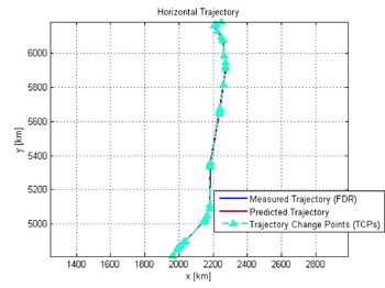
Figure 10. Trajectory prediction, horizontal trajectory.
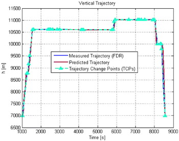
Figure 11. Trajectory prediction, vertical trajectory.
For the predicted trajectory, performance accuracy is now quantified in terms of the EE, ATE, CTE, and RE. The evolution of the EE over time is represented in Figure 12, while the associated Cumulative Distributive Function (CDF) is illustrated in Figure 13. Except for the final part of the trajectory, relevant to the penultimate descending stage, the proposed TP model shows very good performance. Specifically, a mean value of 1·314 km, a standard deviation of 2·270 km and a maximum value of 13·077 km are obtained for the EE. Furthermore, the CDF shows that the EE is less than 2 km in 87% of cases.

Figure 12. Euclidean error between the measured and the predicted trajectory.

Figure 13. Cumulative distribution function for the euclidean error.
A similar behaviour is observed also for the error components ATE, CTE and RE, whose evolution over time is not reported here for the sake of brevity. In line with the whole EE, performance degradation arises only in the final part of the prediction. Furthermore, the ATE is shown to be the component which gives the major contribution to the EE.
The statistics relevant to the EE and to the absolute values of the error components are summarised in Table 2. The CDFs associated with the absolute error components, not reported here in the interest of space, show that, as for the EE, the absolute ATE is less than 2 km in 87% of the cases; on the other hand, the absolute CTE is less than 1 km in 97% of the cases and the absolute RE is less than 100 m (equal to 0·1 km) in 92% of the cases.
Table 2. Performance evaluation relevant to the proposed trajectory prediction model.

As mentioned, the wind-field used in the TP process has been evaluated from a look-up table based on a selection of wind samples. A comparison between the measured wind-field, obtained from the FDR, and the estimated wind-field, derived from the look-up table, is presented in Figure 14 for components w x and w y respectively. The look-up table scheme is equivalent to a nearest interpolation method, and an accurate nominal wind-field is shown to be obtained from the available samples. The vertical component of the wind is always assumed to be negligible, i.e. w z=0.

Figure 14. Wind-field x (Left) and y (Right) components.
8.2. Performance comparison with other methods
As mentioned, two major innovations have been proposed in this work. Firstly, a new procedure for TAS scheduling, able to meet the ETA requirements, is suggested. Secondly, a novel controller for the bank angle input, based on practical pilot procedures, is presented. On the basis of these two innovations, further performance validation has been undertaken by repeating the TP process and using existing methods for the TAS scheduling and/or the bank angle settings. The same FF portion considered in section 8.1, with an extended time-horizon of 7525 seconds and using the same aircraft intent information, has been chosen for such a performance comparison.
Specifically, a first TP reference model sets the desired TAS according to the BADA recommendations. Therefore, the information about the ETA requirements is completely ignored by the model. In addition, the linear controller proposed in the HYBRIDGE project (Glover and Lygeros, Reference Glover and Lygeros2003 and Reference Glover and Lygeros2004) is used for the bank angle settings. On the other hand, a second TP reference model is obtained using the method proposed in this paper for TAS scheduling, so that the model accounts for ETA requirements. However, the bank angle is still set according to the linear controller presented in the HYBRIDGE project (Glover and Lygeros, Reference Glover and Lygeros2003 and Reference Glover and Lygeros2004). The third case adopts the full features of the TP model proposed in this paper, where both proposed methods for TAS and bank angle settings are used. Table 3 presents the results for each of the three scenarios. A significant performance enhancement is observed between the first and the second TP reference model, in which the proposed TAS scheduling is used. When the desired TAS is decided following the BADA recommendations, the shape of the predicted trajectory is shown to be quite similar to that relevant to the actual trajectory. However, the EE, defined as in the equation (14), assumes large values because the aircraft is usually late or early when flying along the predicted trajectory. This is a direct consequence of having ignored the ETA information in the TAS settings. A further performance improvement is also noticed between the second TP reference model and the proposed TP scheme, where the new controller is used to set the bank angle input. By emulating practical pilot procedures, such a controller is shown to be able to quickly reduce the deviations from the RP, thus improving accuracy. Furthermore, only one constant gain needs to be tuned in the linear part of the proposed controller.
Table 3. Performance comparison with existing methods for TAS and bank angle settings.

9. CONCLUSIONS
The importance of accurate TP models is becoming ever more evident in the world of ATM especially in the light of initiatives such as the SESAR programme. TP models currently available in the open literature, whilst complex, have considerable limitations. In this paper, a novel 4D TP model for civil aircraft has been presented. Aircraft intent information, identifying without ambiguity the trajectory to be computed, has been shown to be adequately modelled in the FS, defined as a time-ordered sequence of TCPs. Two major novelties are introduced in this work. Firstly, aircraft lateral guidance is modelled through a new control scheme, based on practical pilot procedures. Secondly, aircraft TAS scheduling is determined in accordance with the ETA requirements. Performance evaluation using FDR obtained from real flight trials in a European Airspace, has shown that the prediction, using the proposed method, is accurate over an extended time-horizon, making it suitable for generating conflict-free trajectories. As the FS can be updated during flight, by adding or changing existing TCPs, airborne Conflict Detection and Resolution (CDR) schemes can be modelled in real time and their effectiveness promptly verified. Further applications of the proposed TP scheme in CDR algorithms will be investigated in a future paper, together with stochastic wind modelling and sensitivity analysis. Furthermore, in order to enhance prediction accuracy, the problem of a better characterisation of the ESF during acceleration or deceleration in both the climb and descent phases of flight will be considered.
APPENDIX: SPECTRAL ANALYSIS
In order to emulate the finite time-response of real systems, the bank angle input generated by the FMS model is processed though a Low Pass (LP) filter, whose design procedure is discussed in this section. Specifically, a first order LP filter is used, and such a choice is motivated by the observation of the FDR relevant to the bank angle. For the same flight used to validate the TP model, the evolution of the bank angle over time is shown in Figure 15. The spectral content of the bank angle signal can be investigated by calculating the associated Fast Fourier Transform (FFT) (Oppenheim and Schafer, Reference Oppenheim and Schafer1975), the amplitude of which is shown in Figure 16. Due to the finite observation time, such a signal is time-limited and, therefore, not band-limited (Oppenheim and Schafer, Reference Oppenheim and Schafer1975). However, an essential bandwidth can be defined as the bandwidth that contains most of the signal energy. By requiring that 99·99% of the energy is saved, an essential bandwidth B ess=0·37404 Hz is obtained.

Figure 15. Bank angle evolution over time from flight data records.

Figure 16. FFT relevant to the bank angle.
As shown in Figure 16, at higher frequencies the envelope of the FFT amplitude decays with a slope of about 20 dB/decade. In general, a similar behaviour can be observed at the output of a first-order LP filter, no matter how noisy the input signal is. For this reason, such a type of filter has been selected to process the bank angle input produced by the FMS model. The cut-off frequency of the filter, f L, is finally determined according to the essential bandwidth of the observed signal, i.e. f L=B ess. The proposed spectral analysis for the bank angle has been repeated also for the FDR relevant to the other flights for which the same aircraft, a Boeing 737-500, was used. For the FFT amplitude, the same behaviour has been observed at higher frequencies. In addition, very similar values have been obtained for the essential bandwidth, and for the cut-off frequency of the LP filter. As a result, such a cut-off frequency can be seen as a further parameter characterising the performance of the aircraft used here.
Provided that the relevant FDR are available, the application of the spectral analysis discussed in this section for the bank angle should be straightforward and equally easy to use to also characterise the other input variables, such as the engine thrust or the flight path angle. According to the analysis results, suitable LP filters can be designed to emulate the actuator systems actually used by aircraft, thus improving TP accuracy.


