


INTRODUCTION
Sandy ocean beaches cover only a small portion of Earth's total surface; and in Brazil, these areas extend along almost all the 9200 km of coastline (Hoefel, Reference Hoefel1998). However, low energy sandy beaches are limited to gulfs, bays, barrier protected lagoons, islands protected by reefs or submerged bars and principally estuaries (Nordstrom, Reference Nordstrom1992; Jackson et al., Reference Jackson, Nordstrom, Eliot and Masselink2002; Goodfellow & Stephenson, Reference Goodfellow and Stephenson2005), which are common in southern and south-eastern Brazil (Borzone et al., Reference Borzone, Melo, Rezende, Vale and Krul2003).
Nordstrom (Reference Nordstrom1992) defines estuarine beaches as sand, gravel or shell beaches located at partially closed places connected to an ocean or sea. In these areas, dominant sediment reworking processes are driven by local waves smaller than 0.25 m (Jackson et al., Reference Jackson, Nordstrom, Eliot and Masselink2002) with the wave formation centre not further than 50 km (Nordstrom, Reference Nordstrom1992; Jackson et al., Reference Jackson, Nordstrom, Eliot and Masselink2002). In addition, beach face widths have to be narrow, measuring less than 20 m in micro-wave regimes, and morphological features must include those inherited by highly energetic events (Jackson et al., Reference Jackson, Nordstrom, Eliot and Masselink2002). Borzone et al. (Reference Borzone, Melo, Rezende, Vale and Krul2003) suggested that these places give rise to a new morphodynamic environment type which is characterized as a transition between wave-dominated sandy beaches and tide-dominated flats.
All morphological features generated by beach peculiarities have influenced the biotic communities of beach environments (Brow & McLachlan, Reference Brown and McLachlan1990; Romer, Reference Romer1990), and many studies have been dedicated to investigate their role in the fish life cycle. These investigations found a numerical prevalence of both few species and juvenile individuals (Lasiak, Reference Lasiak1984, Reference Lasiak1986; Santos & Nash, Reference Santos and Nash1995; Gibson et al., Reference Gibson, Ansell and Robb1993; Clark et al., Reference Clark, Bennet and Lamberth1996; Clark, Reference Clark1997; Strydom, Reference Strydom2003). Most fish remained during short periods in this environment (Gibson et al., Reference Gibson, Ansell and Robb1993) and only a reduced number of species showed annual residence (Brown & McLachlan, Reference Brown and McLachlan1990). Another important factor in beach environment is the high food availability due to continuous wave action, which makes nutrients available in the water column. This process favours phytoplankton enrichment, and consequently, the planktophagic organisms (McLachlan, Reference McLachlan1980).
Previous studies have found greatest fish abundance during warmer months, decreasing with temperature reduction (Modde & Ross, Reference Modde and Ross1981; Ross et al., Reference Ross, McMichael and Ruple1987; Gibson et al., Reference Gibson, Ansell and Robb1993; Santos & Nash, Reference Santos and Nash1995; Clark et al., Reference Clark, Bennet and Lamberth1996). These differences are attributed to the effect of the environmental set, such as wind, wave and water temperature (Lamberth et al., Reference Lamberth, Bennett and Clark1995). However, some authors have found greatest abundances during spring rather than in the summer, as it was expected (Godefroid et al., Reference Godefroid, Hofstaetter and Spach1997; Félix et al., Reference Félix, Spach, Moro, Schwarz, Santos, Hackradt and Hostim-Silva2007a).
Many authors have studied fish communities at Brazilian beaches. The first studies were focused on understanding spatial and temporal community patterns, characterizing species composition and comparing sites (Cunha, Reference Cunha1981; Paiva-Filho et al., Reference Paiva-Filho, Giannini, Ribeiro Neto and miegelow1987; Monteiro-Neto et al., Reference Monteiro-Neto, Blacher, Laurent, Snisck, Canozzi and Tabajara1990; Graça Lopes et al., Reference Graça Lopes, Rodrigues, Puzzi, Pita, Coelho and Freitas1993; Monteiro-Neto & Musick, Reference Monteiro-Neto and Musick1994; Giannini & Paiva-Filho, Reference Giannini and Paiva-Filho1995; Saul & Cunningham, Reference Saul and Cunningham1995; Teixeira & Almeida, Reference Teixeira and Almeida1998; Lopes et al., Reference Lopes, Oliveira-Silva, Sena, Silva, Veiga, Silva and Santos1999; Gomes et al., Reference Gomes, Cunha and Zalmon2003). Most recently, authors have investigated the daily ichthyofaunal variation and the influence of morphodynamic gradients (Gaelzer & Zalmon, Reference Gaelzer and Zalmon2003; Pessanha & Araújo, Reference Pessanha and Araújo2003).
With respect to the coast of Paraná, beach ichthyofauna is poorly studied, with few dispersed investigations, mainly on local comparisons between sandy beaches (Pinheiro, Reference Pinheiro1999), temporal variations (Godefroid et al., Reference Godefroid, Hofstaetter and Spach1997, Reference Godefroid, Spach, Santos, MacLaren and Schwarz2004), ichthyoplankton (Godefroid et al., Reference Godefroid, Hofstaetter and Spach1999) and the influence of morphodynamism on fish community (Félix et al., Reference Félix, Spach, Moro, Hackradt, Queiroz and Hostim-Silva2007b). Estuarine beaches were only evaluated based on species composition (Hackradt et al., Reference Hackradt, Pichler, Félix, Swarz, Silva and Spach2009) and temporal variation (Godefroid et al., Reference Godefroid, Hofstaetter and Spach1997; Félix et al., Reference Félix, Spach, Hackradt, Moro and Rocha2006).
Despite the range of advances in studies of different beach environments and the great number of biological assessments at several estuarine habitats, such as mangroves, seagrass beds, tidal flats and water columns, estuarine beaches remain largely unstudied (Nordstrom, Reference Nordstrom1992; Hoefel, Reference Hoefel1998). They are unique environments that differ from sandy beaches by presenting a stable substrate that allows fauna and flora attachment (Nordstrom, Reference Nordstrom1992). In this context, the aim of the present study is to understand the ichthyofaunal structuring at six estuarine beaches along a salinity–energy gradient inside the largest estuary in southern Brazil.
MATERIALS AND METHODS
Study area
The Bay of Paranaguá is described as a type B, partially-mixed estuary, with lateral heterogeneity (Knoppers et al., Reference Knoppers, Brandini and Thamm1987). The estuary penetrates 50 km into the continent, with a mean width of 10 km and an average depth of 5.4 m (Noernberg et al., Reference Noernberg, Lautert, Araújo, Marone, Angelloti, Netto and Krug2004). The occurrence of a salinity and energy gradient along the east–west axis divides the bay into three zones: (1) an external high energy region with average salinity of about 30, called the euhaline region, which includes the following beaches: Encantadas (EN: 25°33′49.1″S 48°19′05.1″W), Brasília (BR: 25°31′36.4″S 48°20′35.7″W), Coroinha (CO: 25°30′40.9″S 48°22′38.8″W) and Cobras' Island (IC: 25°29′03.1″S 48°25′50.6″W); (2) an intermediary, polyhaline region where Piaçaguera beach is located (PI: 25°29′03.1″S 48°29′40.0″W); and (3) an innermost low energy and salinity region, called the oligo-mesohaline region, with salinity values between zero and 15, where Europinha beach is located (EU: 25°27′39.2″S 48°36′41.1″W) (Figure 1). Usually, waves are originated by south-eastern winds at the estuary mouth region, displaying on average half a metre height and three to seven seconds period duration. In stormy conditions, waves can reach a maximum of 3 m height (Lana et al., Reference Lana, Marone, Lopes, Machado, Seeliger and Kjerfe2001).
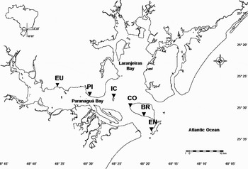
Fig. 1. Paranaguá Bay estuarine complex. Map showing the six studied beaches (EU, Europinha; PI, Piaçaguera; IC, Cobras' Island; CO, Coroinha; BR, Brasília; EN, Encantadas).
Data collection
Fish assemblages at the 6 locations were sampled during daylight hours, between 6.00 and 13.00 h from June 2005 to May 2006, using a beach seine net, 15 m long and 2.6 m height with a stretched mesh size of 5 mm. Three 20-m hauls were made at each site, separated 5 m apart to minimize the influence on the following haul. All sampling campaigns began at neap low tide, following the same beach visiting sequence. Hauls were pulled simultaneously and parallel to the beach face by two persons, one at each end of the net. All fish collected were identified to species level following Figueiredo & Menezes (Reference Figueiredo and Menezes1978, Reference Figueiredo and Menezes1980, Reference Figueiredo and Menezes2000) Fischer (Reference Fischer1978), Menezes & Figueiredo (Reference Menezes and Figueiredo1980, Reference Menezes and Figueiredo1985) and Barletta & Corrêa (Reference Barletta and Corrêa1992). These were then weighed (g) and measured to the nearest 1 mm (total length and standard length), except when samples were very large. On such occasions, measurements were restricted to a subsample of 30 individuals per species. The excess was weighed, counted and incorporated as weight and number counts.
Environmental data were measured concomitantly with beach hauls: surface water salinity (using a refractometer), surface water temperature (through a mercury thermometer), pH (through a portable pH meter), wave height and wave duration. Wave height was taken with a 2-m ruler and obtained from the metric difference between crest and sea level of the largest waves breaking on the surf zone. Wave period was measured from the duration (in seconds) of 11 successive breaking waves divided by 10 to obtain the period of a single wave. This procedure was applied twice to produce an average.
Seasons of the year were defined as follows: summer (December, January and February), autumn (March, April and May), winter (June, July and August) and spring (September, October and November).
Data analysis
To determine whether species can be classified as dominant, the following criteria have been used: frequency of occurrence in the samples exceeding 10%; abundance exceeding 1%; and, constant occurrence, i.e. present in at least eight collection months.
To test whether the abundance (N), number of species (S), catch weight (P), Margalef's richness (d), Pielou's evenness (J′) and Shannon–Wiener diversity (H′) were spatio-temporally different, two-way analysis of variance (ANOVA) (Pielou, Reference Pielou1969; Ludwig & Reynolds, Reference Ludwig and Reynolds1988) was applied. Before conducting the test, biotic data were tested for homoscedasticity and normality by the Bartlett and Kolmogorov–Smirnov tests, respectively (Sokal & Rohlf, Reference Sokal and Rohlf1995). To fulfil ANOVA assumptions, abundance (N), catch weight (P), Pielou's evenness (J′) and Shannon–Wiener diversity index (H′) data were transformed by Log(x + 1). When differences were significant (P < 0.05), the a posteriori Student–Newman–Keuls test was used to identify which averages were different.
Data on species abundance (log transformed) were converted into similarity matrices using the Bray–Curtis similarity index, with all field points separated by seasons. Following, ANOVA results were displayed on a dendrogram using group average linking (cluster), and an ordination plot, generated by a non-metric multidimensional scaling (MDS) procedure (Clarke & Warwick, Reference Clarke and Warwick1994). To evaluate the statistical importance of group formation, a similarity analysis (ANOSIM) was performed and, to reveal species contribution to group formation, a similarity of percentages (SIMPER) procedure was conducted subsequently. To evaluate the correlation level between environmental data that best explained fish community patterns, the BIOENV routine was applied.
RESULTS
Environmental results showed beach singularities and marked temporal differences. Temperature reached highest values during summer months and lowest in early spring, varying equally in space (Figure 2A). Salinity was high during winter and the opposite trend was observed in summer and spring months, with lower values at inner beaches and higher values at outermost areas (Figure 2B). Lowest pH values were found at the most internal beach (Europinha) whilst higher values occurred on beaches at Mel Island (Coroinha, Brasilia and Encantadas). Temporally, larger pH values were registered in November, December and February (Figure 2C). Morphodynamic data, i.e. wave height and period, displayed higher values towards the external beaches and the opposite on the inner beaches. Encantadas showed the highest wave height values (Figure 2D, E) and depth was greatest at Cobras' Island beach (140 cm), followed by Encantadas (90 cm), Brasilia (70 cm), Piaçaguera (65 cm), Coroinha (50 cm) and Europinha (20 cm).
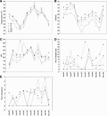
Fig. 2. Environmental data collected at six beaches sampled: (A) temperature in oC; (B) salinity; (C) pH; (D) wave height in centimetres; (E) wave period in seconds.
Ichthyofaunal composition was different amongst the studied beaches. Family and species numbers and number of exclusive species were greater at the intermediate sector, Cobras' Island, decreasing in the direction of the outermost beaches, Europinha and Encantadas. Nonetheless, catch weight displayed a reverse trend, with larger values at the outermost beaches. Abundance was greater at Piaçaguera (5281), Europinha (4607) and Cobras' Island (3303) and smallest at Brasilia (1129) (Table 1). Dominance increased gradually in relation to exposure level, except for a high level of dominance found at Piaçaguera beach (Figure 3).
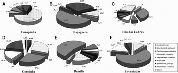
Fig. 3. Dominant species proportion in each of the six beaches studied at Paranaguá Bay, Paraná, Brazil.
Table 1. Species abundance, total relative frequency, preferential habitat and species association to coastal habitat caught at the six beaches studied at Paranaguá Bay, Paraná, Brazil (EU, Europinha; PI, Piaçaguera; IC, Cobras' Island; CO, Coroinha; BR, Brasília; EN, Encantadas; *, dominant species; M, marine; E, estuary; ME, marine and estuary; S, soft bottom; RR, rock reef; WC, water column; ?, information not available; number of exclusive species and families between parentheses). Species are ordered alphabetically.
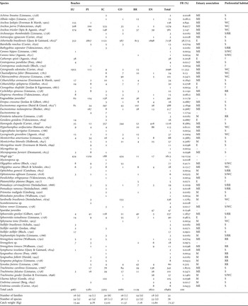
Some beaches have been characterized by dissimilar species occurrences and abundance levels. Although Mugil spp. and Atherinella brasiliensis have been abundant and common in all beaches, they were more representative at Europinha and Piaçaguera, the latter amounting for 80% of the total catch in number. Nevertheless, the occurrence of Centropomus pararellus, Cathorops spixii, Caranx hippos, Stellifer stellifer and Sardinella brasiliensis at Europinha and Scomberomorus sp., Microgobius sp., Ctenogobius shufeldti and Centropomus undecimalis at Piaçaguera, illustrate the differential spatial utilization of the studied beaches by the species. A great number of uncommon species was caught at Cobras' Island beach. The species Paralichthys orbignyanus, Achirus lineatus, Ophichthus gomesii, Rhinobatos percellens, Mycteroperca sp., Stephanolepis hispidus, Pomadasys ramosus, Bathygobius soporator, Fistularia tabacaria, Syngnathus elucens and Lagocephalus laevigatus were caught exclusively at this beach. However, at the exposed beaches (Coroinha, Brasilia and Encantadas), only Sphyraena tome; Platanichthys platana and Caranx latus; Umbrina coroides and Sparidae juveniles occurred exclusively there (Table 1).
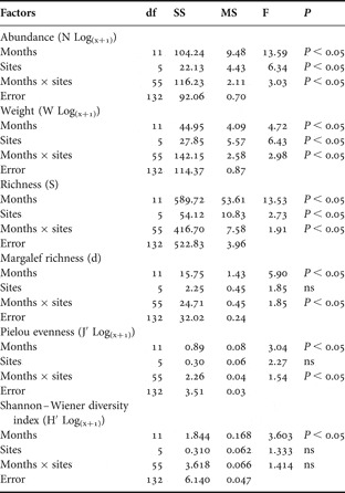
Month and site (beach) factors were considered fixed in the two-way ANOVA. Abundance, species richness, weight, Margalef richness and Pielou evenness data were significant on factors interaction, whilst Shannon–Wiener diversity differed only amongst months (Table 2). According to post-hoc tests, high abundance values were found in February and March, and were different in June and July when lower catches occurred. Spatially higher catches in number, owing to Atherinella brasiliensis and Mugil spp. captures at Piaçaguera, Cobras' Island and Encantadas, caused them to differ from the others beaches (Figure 4A).
Table 2. Analysis of variance of factors influencing the biotic variables. Factors analysed: months, sites and factor interaction. ns, non-significant.
Higher mean weight values were registered during warmer months, which differed statistically from cold ones. Europinha, Piaçaguera and Cobras' Island showed significantly higher average values in December, February, March and May, in contrast to the remaining beaches (Figure 4B). Species richness was always higher in Europinha, Cobras' Island and Encantadas than Piaçaguera and Brasilia, despite the temporal variation, which presented two marked high points, one in September and the second in February and March (Figure 4C).
Ecological indices, Margalef's richness and Pielou's evenness, changed mainly between late winter–early spring and summer due to high contributions from Cobras' Island and Europinha (Figure 4D, E). Shannon–Wiener diversity indices were only different between months, with spring and summer months distinguished from winter ones (Table 2; Figure 4F).
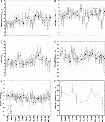
Fig. 4. Analysis of variance plots displaying only significant results for the variables studied. (A) Abundance (log transformed); (B) catch weight (log transformed); (C) number of species (richness) and the ecological indices; (D) Margalef richness; (E) Pielou eveness (log transformed); (F) Shannon–Wiener diversity index (log transformed).
According to ANOVA results, multivariate analysis was conducted considering months grouped within seasons. Despite high values of stress, four groups were formed in each MDS and cluster combination plots. In winter, under 50% of similarity, groups A and B pooled an inner beach (Europinha) and two outermost locations (Coroinha and Encantadas), respectively, whilst groups C and D included intermediate beaches (Figure 5A). ANOSIM showed low significance levels and correlation, 0.207 (Table 3); but according to species occurrence and abundance indicated by SIMPER, internal similarities were greater than 50%, except for group B (22%). In addition, high dissimilarity percentages were found between groups, principally due to contributions from Cathorops spixii, Anchoa parva, Sphoeroide greeleyi, Atherinella brasiliensis, Anchoa tricolor and Harengula clupeola (Table 4).
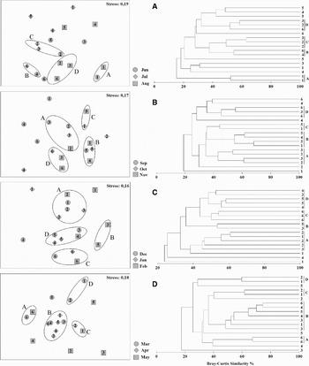
Fig. 5. Multi-dimensional scaling and cluster analysis of the seasons (A, winter; B, spring; C, summer; D, autumm).
Table 3. Analysis of similarities results showing global R values and significance levels for each season.
Table 4. Similarity percentage (SIMPER) analysis within and between groups formed by cluster and multidimensional scaling plots showing the species that most contributed to similarities and dissimilarities, and their respective proportions.

During spring, minor differentiations were observed; group A included Piaçaguera (September and November) and Cobras' Island (September and October), group B pooled November Europinha and Coroinha with September and October Brasilia. Group C also joined Brasilia (November) and Europiunha (October), and the last group, D, included Encantadas (October and November) and Cobras' Island (November) (Figure 5B). A low correlation level between groups was demonstrated by ANOSIM results (0.253) (Table 3). SIMPER analysis exhibited 45% of internal similarity, with the greatest value (58%) at group B. High dissimilarities between groups (always greater than 65%) were attributed to the occurrence and abundance of engraulid juveniles, A. brasiliensis, Mugil spp., Sphoeroides greeleyi, Sphoeroides testudineus, Menticirrhus americanus, Harengula clupeola and Trachinotus carolinus (Table 4).
Greater segregation between beaches was observed in summer, when a lower stress value was observed (0.16) and confounded Cobras' Island with the remaining beaches. Group A consisted of Piaçaguera, Europinha (December) and Cobras' Island (January). Group B was formed by the February Cobras' Island and Brasília and group C only by Encantadas. Group D pooled intermediate beaches: Cobras' Island (December), Coroinha (January and February) and Brasilia (December and January) (Figure 5C). ANOSIM correlation was also higher, 0.449, with high significance level, 60% (Table 3). More than 50% of internal similarity and dissimilarity between groups were observed on SIMPER results, and Mugil spp., Atherinella brasiliensis, Trachinotus carolinus, Eucinostomus argenteus, Sphoeroides greeleyi and Hyporhamphus unifasciatus were the species that most contributed to this pattern (Table 4).
In contrast to summer, autumn was the season when grouping of the beaches was more pronounced and a distinction between internal and external beaches could be noted. Group A joined Encantadas (March and May); group B included samples of all beaches and both groups C and D aggregated Europinha in April and May, and Piaçaguera in March (Figure 5D). Lowest levels of significance (14%) and correlation (0.223) were found according to ANOSIM (Table 3). However, inner similarities and dissimilarities between groups were all around 60%, when occurrence and abundance of Anchoa parva, Mugil spp., Anchoa tricolor, Eucinostomus argenteus, Atherinella brasiliensis, Harengula clupeola, Trachinotus falcatus, Trachinotus carolinus, Strongylura timucu, Trachinotus goodei and Cetengraulis edentulus were responsible for the grouping (Table 4). The latter was particularly important due to a single catch with more than 1900 individuals at Europinha in March.
The BIOENV routine was used to compare environmental data with abundance and distribution of species at the beaches studied. Despite low correlation values displayed by the BIOENV results, the best variable that explained 21% of data variation was depth. Temperature was the second variable that might have influenced species pattern; other variables, when present, decreased the correlation value owing to their negative correlation with biotic data (Table 5).
Table 5. BIOENV results showing the best variables that explain abundance and distribution of species caught at the six estuarine beaches studied.

DISCUSSION
Romer (Reference Romer1990) showed that abundance and diversity are inversely proportional compared to beach exposure degree. However, other factors may affect the fish communities in shallow environments, for instance the availability of micro-habitats (Clark et al., Reference Clark, Bennet and Lamberth1996), e.g. leafy accumulation and submerged vegetation, which increase fish abundance. Cobras' Island beach provided the highest number of families and species. The most probable explanation for this pattern is the presence of distinct adjacent environments, such as rocky coastlines on both sides of the beach and a greater depth, which according to Suda et al. (Reference Suda, Inoue and Uchida2002) promote an increase in number of individuals and species. In addition, that beach presented the only record of typical rocky reef species such as Fistularia tabacaria, Ophichthus gomesii, Mycteroperca sp. and Stephanolepis hispidus, which corroborate the micro-habitat influence hypothesis. This influence is normally linked to small beach width, which attracts species from adjacent habitats, and to morphology, which in the case of Cobras' Island concentrates individuals in the centre of the bay as a result of the shape configuration (Gibson, Reference Gibson1973; Suda et al., Reference Suda, Inoue and Uchida2002).
The species Cathorops spixii and Centropomus undecimalis (exclusively captured at Europinha beach), the large number of soles captured, Citharichthys spilopterus and Citharichthys arenaceus, and the additional records of Genidens genidens, Stellifer rastrifer and Centropomus parallelus, showed the influence of mudflats on this beach which was expressed by the presence of typical estuarine species (Gomes et al., Reference Gomes, Cunha and Zalmon2003). Despite the existence of mudflats on the other beaches, its large extension and composition seem to have greater influence on species composition than beach profile alone.
Although captured on almost all beaches studied, the carangid species Trachinotus carolinus and Trachinotus falcatus were more abundant at Cobras' Island, Coroinha, Brasília and Encantadas, whilst Trachinotus goodei was only associated with Brasília and Encantadas. These are recognized as sandy beach species (Modde, Reference Modde1980) and thus, beaches closer to the bay entrance show greater similarity with adjacent oceanic beaches. Trachinotus falcatus has already been recorded in the innermost areas of the estuarine complex, in the oligohaline sector of the Antonina Bay (Spach et al., Reference Spach, Félix, Hackradt, Laufer, Moro and Catani2006), whilst the other species of the genus seem to be restricted to the outermost areas (Vendel et al., Reference Vendel, Lopes, Santos and Spach2003; Spach et al., Reference Spach, Godefroid, Santos, Schwarz and Queiroz2004).
The beaches studied showed dominance of few species according to the criteria determined in this study, which is expected for beach environments (McFarland, Reference McFarland1963; Modde & Ross, Reference Modde and Ross1981; Ross et al., Reference Ross, McMichael and Ruple1987; Santos & Nash, Reference Santos and Nash1995; Godefroid et al., Reference Godefroid, Spach, Santos, MacLaren and Schwarz2004) and shallow estuarine areas (Kennish, Reference Kennish1986; Santos et al., Reference Santos, Schwarz, Oliveira-Neto and Spach2002). Worldwide studies on sandy beaches demonstrated that dominance increases proportionally with increases in exposure to energy gradient (Romer, Reference Romer1990; Clark et al., Reference Clark, Bennet and Lamberth1994; Clark, Reference Clark1997; Gaelzer & Zalmon, Reference Gaelzer and Zalmon2003). This was evidenced by the increase in exposure levels towards beaches next to Paranaguá bay entrance and the concomitant dominance increase. Although Piaçaguera beach is located in front of Paranaguá harbour (and, therefore, in an intermediary position in relation to the degree of exposure) a high dominance was detected. This factor could be explained by the removal of rare individuals from the population (Clarke & Warwick, Reference Clarke and Warwick1994) due to stress resulting from harbour activities.
Analyses of weight, number of individuals and species and ecological indices data showed distinctions between the beaches in time and space. Notable differences occurred between the seasons, and summer showed the greatest captures in abundance and number of species. Such a pattern could be associated with the congruence of the reproductive period of many species and the great availability of food provided by an increase in the plankton (the base of the food chain), making more food available for plankton feeders (Kennish, Reference Kennish1986). Weight varied considerably due to the capture of large-sized samples at the deepest beaches and to the sporadic catch of large shoals. Margalef's richness and Pielou's evenness varied in temporal and spatial scales, owing to a greater heterogeneity in assemblage distribution during winter and spring (Nash & Santos, Reference Nash and Santos1998). However, Shannon–Wiener diversity only displayed temporal differences due to the fluctuation in species number and abundance between the seasons. In fact, the dominant species are always the same, only alternating their rank position in frequency, abundance and weight (Modde & Ross, Reference Modde and Ross1981). As a result, the more stable an environment is the stronger the trend for higher values of diversity and evenness (Dexter, Reference Dexter1984).
Owing to ANOVA results, a multivariate analysis was conducted by grouping sampled months into seasons. Further evidence that corroborated the spatial variability amongst the beaches studied was from the multidimensional scaling analysis which revealed a general tendency in the beach groups. Europinha and Encantadas were distinct from the remaining beaches, with the former being more similar in species composition to other tidal flats studied throughout the estuary (Santos et al., Reference Santos, Schwarz, Oliveira-Neto and Spach2002; Vendel et al., Reference Vendel, Spach, Lopes and Santos2002) and the latter showing an ichthyofauna similar to those described on the adjacent oceanic beaches (Godefroid et al., Reference Godefroid, Spach, Santos, MacLaren and Schwarz2004; Félix et al., Reference Félix, Spach, Moro, Schwarz, Santos, Hackradt and Hostim-Silva2007a).
In spite of the spatial and temporal distinctions in the two analyses conducted, one factor should be taken into consideration when interpreting these differences. The random catch of the fishing gear could influence the results of the uni- and multivariate analyses, reflecting in grouping of some hauls from different beaches in certain sampling months. A further interesting factor is the elevated stress observed in the ordination analysis, which suggests that the graphic distances may not adequately represent the original similarities. Due to data logarithmic transformations, the actual differences or the lack of them may have been further masked. ANOSIM has also shown low correlation values between formed groups, with summer being an exception. Nevertheless, even considering the factors mentioned above, the beaches behaved differently and they were distinct for most of the time.
Abrupt variations in salinity, temperature, oxygen and turbidity are common in estuarine regions and are caused by the influence of tides and mixture between fresh and seawater (Kennish, Reference Kennish1986). The rapid variations in physical, chemical and biological properties require a great demand of energy for biological components from these locations (Day et al., Reference Day, Hall, Kemp and Yañez-Arancibia1989). A tendency for higher values of the abiotic factors towards the bay entrance was observed in the studied areas. According to the results of the BIOENV analysis used to explain that the ichthyofaunal raise composition and distribution in relation to the environmental variables, we observed that amongst the variables analysed, those providing the most expressive contribution in small scale were depth and temperature. However, additional data on beach profile and its comparison to morphodynamic data are necessary to improve our understanding of the environmental influence on the ichthyofauna of low energy beaches.
In general, spatial differences found between beaches in this study could be explained by a sum of factors. The morphodynamic characteristics that figure as fundamental in fish community structure in oceanic beaches (Dye et al., Reference Dye, McLachlan and Wooldridge1981; Lasiak, Reference Lasiak1984; Romer, Reference Romer1990; Clark et al., Reference Clark, Bennet and Lamberth1994, Reference Clark, Bennet and Lamberth1996; Clark, Reference Clark1997) may be considered secondary in estuarine beaches. Nonetheless, these characteristics should not be disregarded since beaches displayed differences in species occurrence and occupation patterns, and the factors describing beach environments may have influenced that variation. Factors such as high wave heights and periods on external beaches (Romer, Reference Romer1990; Gaelzer & Zalmon, Reference Gaelzer and Zalmon2003; Félix et al., Reference Félix, Spach, Moro, Hackradt, Queiroz and Hostim-Silva2007b) may create an energy-gradient, which increases towards the bay entrance direction (Lana et al., Reference Lana, Marone, Lopes, Machado, Seeliger and Kjerfe2001). However, differences on beach features seem to be the main factors influencing the ichthyofauna, because the energy of oligohaline and mesohaline regions has shown limited influence. Moreover, depth showed significant differences on species distribution.
Another factor that might be influencing is the presence of adjacent habitats like rocky coasts and muddy flats (Clark et al., Reference Clark, Bennet and Lamberth1996; Suda et al., Reference Suda, Inoue and Uchida2002). Different features like adjacent habitat influence, distinct substrate composition and human activities appear to have a great potential to influence the beaches studied. However, to make any conclusion on which factors truly determine the observed patterns and how much they influence, sampling schemes designed to solve the influence of factors must be properly planned and the use of spatial replicates should be emphasized (Underwood, Reference Underwood1997).


