


INTRODUCTION
Species composition of wild reservoir hosts can influence the transmission and maintenance of multi-host vector borne pathogens. In theory, life history characteristics among species within a community can be an important driver of variation in infectious disease transmission (Lochmiller and Deerenberg, Reference Lochmiller and Deerenberg2000; Martin et al. Reference Martin, Weil, Kuhlman and Nelson2006; Miller and Sinervo, Reference Miller and Sinervo2007; Johnson et al. Reference Johnson, Rohr, Hoverman, Kellermanns, Bowerman, Lunde, DiAngelo, Bland, Bambina, Cherry and Birnbaum2012). Relative to infectious disease transmission, the ‘pace of life’ hypothesis posits that r-selected species, those that have high reproductive rates and with relatively short lifespans, are expected to invest less in acquired immunity compared with species that are more ‘k-selected’, with lower reproductive rates and longer life spans (Martin et al. Reference Martin, Weil, Kuhlman and Nelson2006; Lee et al. Reference Lee, Wikelski, Robinson, Robinson and Klasing2008). Furthermore, highly reproductive (r-selected) species tend to have higher litter sizes and give birth more frequently, leading to an increased number of susceptible individuals, which can lead to increased rates of infectious disease transmission in a population (Poulin and Morand, Reference Poulin and Morand2004; Blackwell et al. Reference Blackwell, Snodgrass, Madimenos and Sugiyama2010). Therefore, among a community of hosts, ‘fast-paced’ species may be more competent reservoirs of infection than ‘slow-living’/‘longer-lived’ species (Ostfeld et al. Reference Ostfeld, Levi, Jolles, Martin, Hosseini and Keesing2014).
The ‘pace of life’ hypothesis in nature has been evidenced in a variety of wildlife-parasite systems. In amphibians, Johnson et al. (Reference Johnson, Preston, Hoverman and Richgels2013), observed that ‘fast-lived’ amphibian species were more susceptible to infection and had more severe pathology associated with trematode infections (Johnson et al. Reference Johnson, Preston, Hoverman and Richgels2013). Regarding vector-borne diseases, Borellia burgdorferi (Lyme disease agent) reservoir competence (the host ability to infect uninfected ticks) was highest in the most r-selected species and lower in more slowly reproducing species (Previtali et al. Reference Previtali, Ostfeld, Keesing, Jolles, Hanselmann and Martin2012; Ostfeld et al. Reference Ostfeld, Levi, Jolles, Martin, Hosseini and Keesing2014). Models evaluating reservoir host traits show that host life history traits such as lifetime reproductive output, are also an important predictor of zoonotic disease reservoir potential (Han et al. Reference Han, Schmidt, Bowden and Drake2015).
In this study, we model how species composition in five different habitats characterized by different degrees of anthropogenic disturbance impacts vector and host infection with Trypanosoma cruzi, the cause of Chagas disease in humans. Chagas disease is a neglected zoonotic, vector-borne tropical disease that infects over 8 million humans worldwide and is a significant cause of morbidity and mortality throughout Central and South America (Bern et al. Reference Bern, Kjos, Yabsley and Montgomery2011). This parasite cycles between a wide range of mammal reservoirs and hematophagous triatomine vectors by multiple routes of transmission. Vectorial transmission is the most known route; however, vector ingestion by hosts seems to be the most efficient dispersion strategy of T. cruzi in sylvatic habitats (Yoshida, Reference Yoshida2008, Reference Yoshida2009; Jansen et al. Reference Jansen, Xavier and Roque2015). The congenital route is relevant in humans (Carlier et al. Reference Carlier, Sosa-Estani, Luquetti and Buekens2015) and under experimental conditions in multiple mammal species infection (Alkmim-Oliveira et al. Reference Alkmim-Oliveira, Costa-Martins, Kappel, Correia, Ramirez and Lages-Silva2013). Finally, laboratory studies have reported direct transmission between triatomines (Ryckman, Reference Ryckman1951; Marinkelle, Reference Marinkelle1965; Añez, Reference Añez1982; Schaub, Reference Schaub1988) and positive serological tests in hyper-carnivorous Felidae suggest transmission between hosts by predation (Rocha et al. Reference Rocha, Roque, de Lima, Cheida, Lemos, de Azevedo, Arrais, Bilac, Herrera, Mourão and Jansen2013); although both infection routes remain a matter of debate (Roellig et al. Reference Roellig, Ellis and Yabsley2009).
The most important host and vector species responsible for T. cruzi transmission varies in different geographical, ecological and epidemiological contexts. Regardless, in many T. cruzi transmission systems, sylvatic cycles can dominate parasite transmission, particularly in rural landscapes or forest-urban boundaries. Our mathematical model of T. cruzi transmission is based on previous data collected from rural landscapes of Panama (Gottdenker et al. Reference Gottdenker, Chaves, Calzada, Saldaña and Carroll2012), where evidence suggests that habitat type (degree of deforestation) and host community composition are important drivers for vector infection prevalence with T. cruzi. Specifically, we incorporate biologically realistic aspects of sylvatic infection into our model, including acute and chronic infection status in hosts, host predation on vectors, and host vertical transmission to better understand their relative importance in T. cruzi transmission and to identify critical parameters to measure in field research.
METHODS
We developed a mathematical model that assumes the basic dynamics of sylvatic T. cruzi transmission cycle, with five coupled ordinary differential equations. We considered vector and mammal hosts, both partitioned into susceptible and infected populations. Additionally, we included a chronically infected population for hosts. We maintained a constant population size where birth rate equals death rate. Figure 1 shows the populations considered in the model with their interactions.
Fig. 1. Model diagram of Trypanosoma cruzi sylvatic system. The model considers vector (S v, I v) and host populations (S h, I h, C h), with their vital dynamics and interactions. For parameters description see Table 2.
Vector dynamics
The vector population is defined by N v and is divided into two compartments: susceptible (S v) and infected (I v). Vectors are born at a per capita rate λ v that is equal to death rate. S v moves into I v by biting infected hosts (I h) or chronically infected hosts (C h), and is described by a Holling type II functional response (Table 1);
 $$g(I_{\rm h}) = \displaystyle{{\varepsilon I_{\rm h}} \over {\rho + I_{\rm h}}}$$
where ε is the maximum number of hosts bitten per week per vector and ρ is the proportion of hosts when host bitten is ε/2.The infection probability of the susceptible vector population is β if the encounter is with infected host class and γ if the encounter is with the chronically infected host population. Parasite transmission from chronically infected hosts to vectors is less likely compared with transmission from the acutely infected host population, thus β ≫ γ. Biological parameters with their values and units are summarized in Table 2.
 $$\eqalign{\displaystyle{{{\rm d}S_{\rm v}} \over {{\rm d}t}} = \lambda _{\rm v}(S_{\rm v} + I_{\rm v}) - \beta g(I_{\rm h})S_{\rm v} - \gamma g(C_{\rm h})S_{\rm v} - \lambda _{\rm v}S_{\rm v}}$$
 $$\displaystyle{{{\rm d}I_{\rm v}} \over {{\rm d}t}} = \beta g(I_{\rm h})S_{\rm v} + \gamma g(C_{\rm h})S_{\rm v} - \lambda _{\rm v}I_{\rm v}$$
Host dynamics
We considered that host population N h is constant, thus birth rate λ h is equal to death rate. In the model the main transmission route by which wild hosts become infected is ingestion of an infected vector. Therefore, susceptible hosts (S h) get infected by feeding on infected vectors (I v) and the probability of infection by this route is defined by η. Host predation on vector population is described by a Holling Type II functional response;
 $$f\,(I_{\rm v}) = \displaystyle{{\phi I_{\rm v}} \over {\sigma + I_{\rm v}}}$$
where ϕ is the maximum number of vectors eaten per week per host and σ represents the proportion of vectors when vector consumption is ϕ/2. Therefore, σ = 0.5 means that host consumption rate on infected vectors is the half (ϕ/2) when 50% of the vectors are infected. In addition, the model assumes that non-insectivorous hosts become infected only by a vectorial route using the same expression, but modifying ϕ to reflect the adequate rate of transmission, thus ϕ depends on species diet.
After an infectious period (α), the infected host population (I h) moves into a chronically infected class (C h). Parameters are described in Table 2. λ h and α depend on the particular host species life history strategy (see Supplementary material).
 $$\displaystyle{{{\rm d}S_{\rm h}} \over {{\rm d}t}} = \lambda _{\rm h}(S_{\rm h} + I_{\rm h} + C_{\rm h}) - \eta f\,(I_{\rm v})S_{\rm h} - \lambda _{\rm h}S_{\rm h}$$
 $$\displaystyle{{{\rm d}I_{\rm h}} \over {{\rm d}t}} = \eta f\,(I_{\rm v})S_{\rm h} - \alpha I_{\rm h} - \lambda _{\rm h}I_{\rm h}$$
 $$\displaystyle{{{\rm d}C_{\rm h}} \over {{\rm d}t}} = \alpha I_{\rm h} - \lambda _{\rm h}C_{\rm h}$$
Host community composition: life history strategy and diet parameters
We modelled the epidemiological dynamics of five habitat types across different degrees of anthropogenic disturbance common in neotropical landscapes, namely contiguous forest, early secondary forest fragment, mid secondary forest remnant, pasture and peridomicile. For each habitat we know about the host species composition based on insect blood meal data collected in the Panama Canal (Gottdenker et al. Reference Gottdenker, Chaves, Calzada, Saldaña and Carroll2012) (Fig. 2). Thus, for each habitat we had different model parameters.
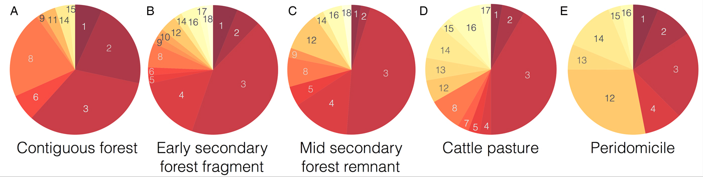
Fig. 2. Proportion of blood meals taken from different species per habitat from Gottdenker et al. (Reference Gottdenker, Chaves, Calzada, Saldaña and Carroll2012). Each number inside the pie chart represents a species coded as follows: 1 – Alouatta palliata, 2 – Cebus capucinus, 3 – Choloepus hoffmanni, 4 – Bos taurus, 5 – Coendou sp., 6 – Potos flavus, 7 – Cyclopes didactylus, 8 – Tamandua tetradactyla, 9 – Sciurus sp, 10 – Heteromyidae sp, 11 – Mustela sp, 12 – Metachirus nudicaudatus, 13 – Sus scrofa, 14 – Didelphis marsupialis, 15 – Philander opossum, 16 – Canis familiaris, 17 – Marmosa sp and 18 – Mus musculus. Species within the pie charts are ordered and colored from the lowest (1 dark red – A. palliata) to the largest birth rate (18 light yellow – M. musculus). Note how the proportion of blood meal coming from species that are more prone to spend time close to dwellings increases as ones moves from the sylvatic to domestic cycle.
Table 1. Variables of the model

Table 2. Model parameters
a These parameters correspond to the Holling Type II functional response.
b Insectivorous hosts: 1–2 ind/week×ind;depending on preference for insects vs. other food sources, non-insectivorous hosts: 0·1 ind/week×ind; to reflect only vectorial transmission.
We considered that host birth rate (λ h), the rate at which infected hosts become chronically infected (α) and diet (ϕ) are the most relevant parameters in our epidemiological model when moving from one species to another. λ h and α are associated with species life history strategy, where α is a measure of the host ability to generate an acquired immune response and it is correlated with a particular species life history strategy. ϕ depends on whether insects have been reported to be part of host dietary intake, thus the parameter varies from one host species to another (for information about host species diet and ϕ values see Supplementary material). Therefore, insectivorous hosts were assumed to ingest 1–2 insects per week depending on preference for insects over other food sources and non-insectivorous hosts 0·1 insects per week to reflect only vectorial transmission. The transmission probability per contact with an infected triatomine has been reported to be between: 10−4 − 10−2 (Rabinovich et al. Reference Rabinovich, Wisnivesky-Colli, Solarz and Gürtler1990, Reference Rabinovich, Schweigmann, Yohai and Wisnivesky-Colli2001; Catala et al. Reference Catala, Gorla and Basombrio1992; Basombrío et al. Reference Basombrío, Gorla, Catalá, Segura, Mora, Gómez and Nasser1996; Nouvellet et al. Reference Nouvellet, Dumonteil and Gourbière2013).
Therefore, the infection probability by the vectorial route is lower compared with the oral route.
The product of species litter size and breeding frequency results in λ h (see Supplementary material). α for all species is difficult to obtain from the literature. However, based on the average parasitaemia reported for Didelphis marsupialis and mice after T. cruzi experimental inoculation, and considering a more robust acquired immunity for longer-lived hosts, we assumed α values for all the species. Host species with birth rates higher than 0 · 09/week, such as D. marsupialis and Mus musculus, were considered as r-selected in a host community and the period of moving from infected (high parasitemia) to chronically infected (low parasitemia) is 12 weeks, or α equals to 1/12 weeks (Jansen et al. Reference Jansen, Leon, Machado, da Silva, Souza-Leão and Deane1991; Añez et al. Reference Añez, Martens, Romero and Crisante2011). On the other hand, host species with birth rate values less than 0 · 01/week correspond to K-selected and α equals to 1/4 weeks. If λ h is between 0·01 and 0·09/week, α equals 1/8 weeks. See Supplementary material for values and references on species individual parameters.
To simulate species composition for each habitat, we estimated λ h, α and ϕ by bootstrapping the distributions reported by Gottdenker et al. (Reference Gottdenker, Chaves, Calzada, Saldaña and Carroll2012) illustrated in Fig. 2. In particular per habitat, we generated 1000 samples by re-sampling with replacement the original distribution. Bootstrapping was conducted to increase variability and compensate for possible field sample bias. Thus, every habitat has an average composite life history strategy based on the species present; this average is marked on Fig. 3 as the mean of the distributions. For each sample distribution we solved the model to steady state (260 weeks/5 years) and recorded the values of the state variables (i.e. proportion of infected hosts and vectors). The initial conditions of the model were: S v = 0 · 9, I v = 0 · 1, S h = 0 · 9, I h = 0 · 1 and C h = 0; however, the steady-state results are independent from the initial conditions. The distribution of the parameters empirically obtained after the simulations for each habitat are shown on Fig. 3.
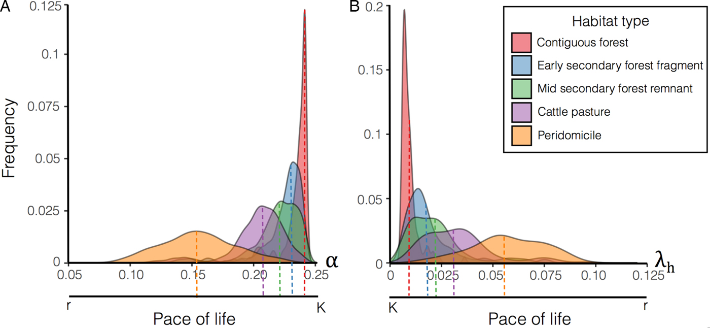
Fig. 3. Distribution of host life history strategy related parameters: α (movement rate from acute to chronically infected) and λ h (birth rate). The frequency distribution for α and λ h is plotted colour-coded per habitat for 1000 samples. Bootstrapping the proportion of blood meals taken from different species (Fig. 1), we obtained 1000 different arrangements per habitat. Each species 1/α and λ h estimates are based on previous reports and life history strategy (see Supplementary material), therefore for each model simulation we used the average value of α and λ h obtained from the resampled ensemble. α is higher in forests compared with other habitats because host community tends to last shorter periods of time in the acute state probably due to a more robust acquired immunity of the longer lived hosts, similarly λ h is higher in peridomicile due to higher litter size and shorter inter-birth intervals.
Model variation: including host vertical transmission route
We incorporated congenital transmission in hosts. The equations describing host population dynamics are amended as follows:
 $$\displaystyle{{{\rm d}S_{\rm h}} \over {{\rm d}t}} = \lambda _{\rm h}S_{\rm h} - \eta f\,(I_{\rm v})S_{\rm h} - \lambda _{\rm h}S_{\rm h}$$
 $$\displaystyle{{{\rm d}I_{\rm h}} \over {{\rm d}t}} = \lambda _{\rm h}(I_{\rm h} + C_{\rm h}) + \eta f\,(I_{\rm v})S_{\rm h} - \alpha I_{\rm h} - \lambda _{\rm h}I_{\rm h}$$
 $$\displaystyle{{{\rm d}C_{\rm h}} \over {{\rm d}t}} = \alpha I_{\rm h} - \lambda _{\rm h}C_{\rm h}$$
Note that if an infected (I h) or chronically infected host (C h) produces offspring in the infected compartment, λ h(Sh + C h). A total of 1000 resamples were generated per habitat type and the model was run until steady state (260 weeks/5 years). The initial conditions of the model were: S v = 0 · 9, I v = 0 · 1, S h = 0 · 9, I h = 0 · 1 and C h = 0, and the proportion of infected populations per habitat was recorded.
Finally, considering that the probability of infection of a S v by a I h is 0·465 (β) and it is an estimate for Rhodnius prolixus feeding on acute guinea pigs (Perlowagora-Szumlewicz et al. Reference Perlowagora-Szumlewicz, Muller and Moreira1990) and similarly the probability of infection of a S v by a C h is 0·026 (γ) and was calculated from a experiment in which Triatoma infestans feeds on seropositive humans (Gurtler et al. Reference Gurtler, Cecere, Castanera, Canale, Lauricella, Chuit, Cohen and Segura1996), we decided to also test the model with increased probabilities (β high, γ high) to account for more competent hosts (Orozco et al. Reference Orozco, Enriquez, Cardinal, Piccinali and Gürtler2016) see Table 2.
The model was implemented using R version 3.3.2 (R Development Core Team, 2016) and the RStudio Integrated Development Environment (IDE). The ordinary differential equations were solved using the ‘deSolve’ package (Soetaert et al. Reference Soetaert, Meysman and Petzoldt2010) and bootstrapping was conducted using the sample function, ‘base’ package version 3.3.2.
RESULTS
Analysis of the model
The basic reproduction number R 0 is the average number of infections produced by the contribution of the whole network. It is a valuable quantity because it tells whether the infection is going to prevail (R 0 ⩾ 1) or disappear and can be used to compare different scenarios. We found R 0 by identifying the largest eigenvalue of Next Generation Matrix method (NGM) (Diekmann et al. Reference Diekmann, Heesterbeek and Metz1990, Reference Diekmann, Heesterbeek and Roberts2010). The NGM has the number of new infected individuals of a class (columns) generated by the introduction of an infected individual of every other class (rows). Thus, for building the NGM, we only consider three of five compartments of our system belonging to infected stages (I v,I h and C h).
 $${\rm NGM} = \left( {\matrix{ 0 & {\displaystyle{{\beta \varepsilon} \over {\rho (\alpha + \lambda _{\rm h})}} + \displaystyle{{\alpha \varepsilon \gamma} \over {\lambda _{\rm h}\rho (\alpha + \lambda _{\rm h})}}} & {\displaystyle{{\varepsilon \gamma} \over {\lambda _{\rm h}\rho}}} \cr {\displaystyle{{\phi \eta} \over {\sigma \lambda _{\rm h}}}} & 0 & 0 \cr 0 & 0 & 0 \cr}} \right)$$
See Supplementary material for more information about NGM construction.
From this product, the greatest eigenvalue is the basic reproductive number.
 $$R_0 = \sqrt {\displaystyle{{\varepsilon \phi \eta (\beta \lambda _{\rm h} + \alpha \gamma )} \over {\sigma \rho \lambda _{\rm v}\lambda _{\rm h}(\alpha + \lambda _{\rm h})}}} $$
To understand the parameter effects on model output, we performed a sensitivity analysis for R 0 using the Latin Hypercube method (LH). Negative values indicate that an increase in a particular parameter determines a decrease in R 0 and positive values an increase in R 0. Therefore, increases in β, γ, η, ϕ and ε generate increments in R 0 (Fig. 4). η(PRCC = 0 · 7), ϕ(PRCC = 0 · 7) and ε(PRCC = 0 · 7) have the higher effect on R 0. In addition, the transmission rate from infected hosts to susceptible vectors (β) has a significant effect (PRCC = 0 · 5). On the other hand, the parameter that has the most significant effect on lowering R 0 is the host birth rate (λ h, PRCC = −0 · 5).
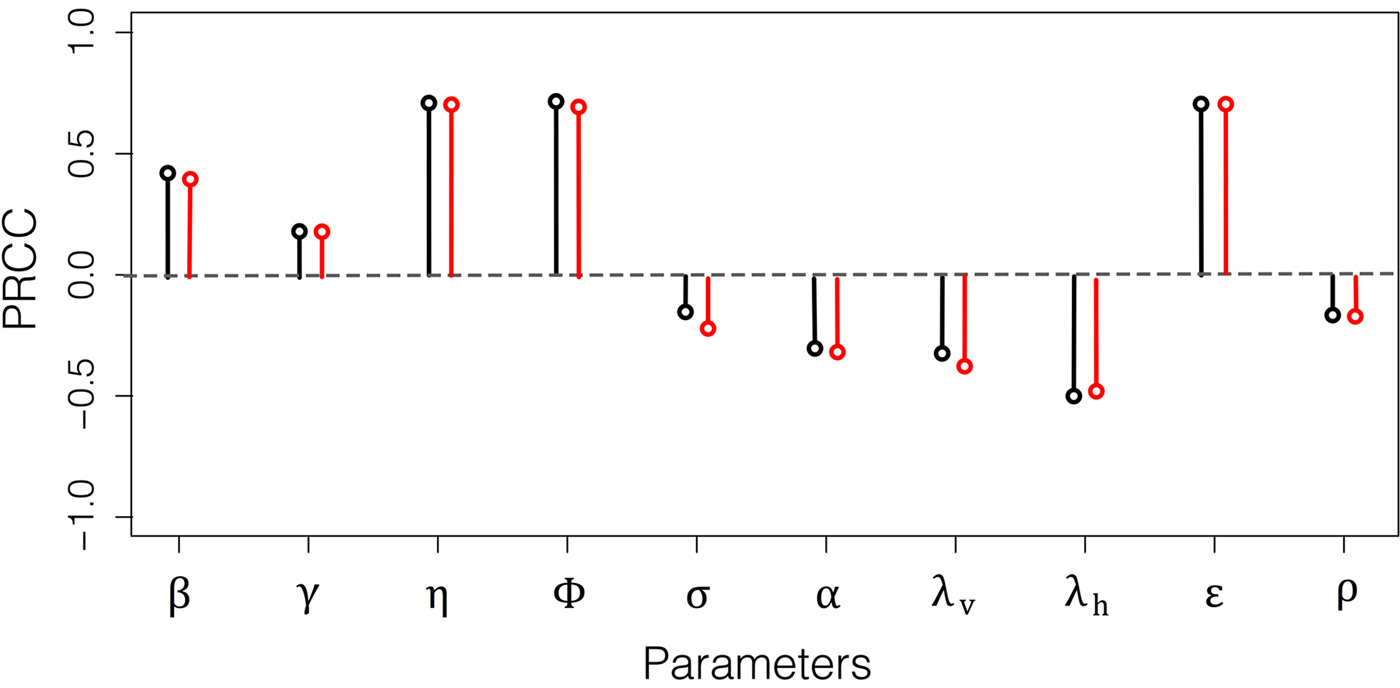
Fig. 4. Latin Hypercube Sampling using the global reproductive number R 0 as model output. PRCC: Partial Rank Correlation Coefficient. Black coloured circles correspond to the model without horizontal transmission and red to the model including host vertical transmission. For information about each parameter's meaning see Table 2. Note that parameters related to host predation on vectors (η and ϕ), vector biting on hosts (ε), and host life history strategy (λ h) have significant and opposite contributions to R 0.
Effect of species composition on the proportion of infected individuals
Each habitat blood meal distribution was resampled 1000 times. We ran the model until it reached steady state (260 weeks/5 years) and record the proportion of infected individual (host and vectors) per habitat. The proportion of infected vectors has the lowest prevalence in the contiguous forest with an I
v = 0 · 121(0 · 118 − 0 · 124). Whereas in the early secondary forest fragment (I
v = 0 · 142, 0 · 138 − 0 · 146), mid-secondary forest remnant (I
v = 0 · 16, 0 · 155 − 0 · 165), pasture (I
v = 0 · 224, 0 · 219 − 0 · 229) and peridomicile (I
v = 0 · 36, 0 · 355 − 0 · 365), the proportion is significantly higher (P <0 · 05) compared with the contiguous forest (Welch two sample t-test
 $95\% \;{\rm CI}$
, Fig. 5).
$95\% \;{\rm CI}$
, Fig. 5).
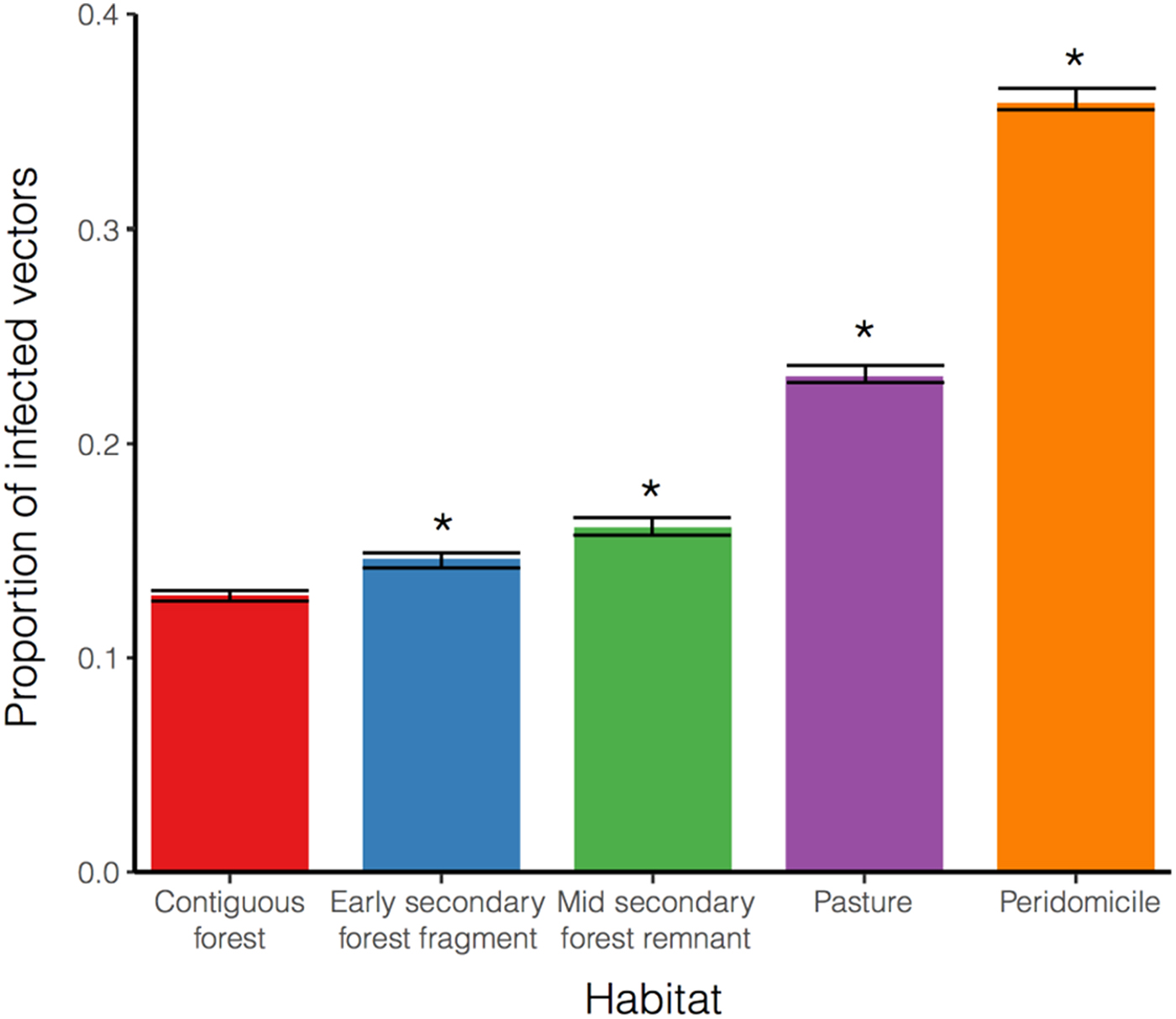
Fig. 5. Proportion of infected vector population (I
v) per habitat at steady state. Results are shown for contiguous forest, early secondary forest fragments, mid secondary forest remnant, pasture and peridomicile. Bar heights represent the average for the 1000 runs and the error bar shows the 95% of confidence interval. *Significant differences compared to contiguous forest (Welch Two Sample t-test,
 $95\% \;{\rm CI}$
). Habitats with forest components (three bars on the left) have an I
v less than 20%, being the contiguous forest the lowest I
v, while the more intervened (two on the right) are well above 20%. Note also that infected vector population has an increasing trend as habitat alteration increases.
$95\% \;{\rm CI}$
). Habitats with forest components (three bars on the left) have an I
v less than 20%, being the contiguous forest the lowest I
v, while the more intervened (two on the right) are well above 20%. Note also that infected vector population has an increasing trend as habitat alteration increases.
Similarly, I h has the same tendency as I v, being the contiguous forest the lowest I h (0 · 021, 0 · 019 − 0 · 022) and the peridomicile the highest among all habitats (I v = 0 · 163, 0 · 159 − 0 · 167). The proportion of infected hosts in the early secondary forest (I h = 0 · 031, 0 · 029 − 0 · 033), mid secondary forest (I h = 0 · 039, 0 · 036 − 0 · 041) and pasture (I h = 0 · 066, 0 · 063 − 0 · 069) is significantly different (P <0 · 05) from the I h in the contiguous forest (not shown).
Vertical transmission in hosts
The model including vertical transmission showed higher proportion of infected vectors for each habitat compared with the model without this transmission mode. As before, the contiguous forest showed the lowest proportion of infected vectors (I v = 0 · 199, 0 · 195 − 0 · 203) and the peridomicile the highest proportion of infected vectors(I v = 0 · 445, 0 · 441 − 0 · 449). Consequently, regarding host population infection, the lowest proportion was reported for the contiguous forest (I h = 0 · 045, 0 · 043 − 0 · 047) and the highest proportion for the peridomicile (I h = 0 · 271, 0 · 265 − 0 · 277).
By increasing the values for β and γ(β high, γ high) the model including vertical transmission better approached field data. Similarly to previous results, the contiguous forest presented the lowest proportion of infected vectors (I v = 0 · 402, 0 · 398 − 0 · 406); followed by the secondary forests (early secondary forest fragment I v = 0 · 460, 0 · 455 − 0 · 465; mid secondary forest remnant I v = 0 · 482, 0 · 477 − 0 · 487) pasture (I v = 0 · 552, 0 · 548 − 0 · 556) and peridomicile (I v = 0 · 646, 0 · 642 − 0 · 650). Infected host population exhibited the same pattern, the proportion of infected hosts in the contiguous forest was (I h = 0 · 046, 0 · 044 − 0 · 048) and in the peridomicile (I h = 0 · 271, 0 · 265 − 0 · 277).
DISCUSSION
Here, we present an epidemiological model that investigates the transmission dynamics of T. cruzi in five different sylvatic environments in the Panama Canal with different anthropogenic intervention levels influencing host communities. Our model shares many features with previous theoretical studies. For instance, studies like the one by Spagnuolo et al. (Reference Spagnuolo, Shillor and Stryker2011) that investigate the effect of spraying dwellings on disease endemicity (Spagnuolo et al. Reference Spagnuolo, Shillor and Stryker2011), or other research teams studying the role of dogs (Fabrizio et al. Reference Fabrizio, Schweigmann and Bartolini2016) and synanthropic animals in human infection (Peterson et al. Reference Peterson, Bartsch, Lee and Dobson2015), also use traditional compartmental epidemiological models. Other studies like Coffield in 2013 and Kribs-Zaleta in 2010 used Holling functions to simulate host predation on vectors (Kribs-Zaleta, Reference Kribs-Zaleta2010; Coffield et al. Reference Coffield, Spagnuolo, Shillor, Mema, Pell, Pruzinsky and Zetye2013). Therefore, we feel confident that the model proposed here can be a simple, yet powerful tool to understand the role of host community composition in sylvatic T. cruzi transmission cycles.
In addition to being a good tool, the model also adjusts to real data. When comparing the proportion of Rhodnius pallescens infected with T. cruzi predicted by the model without vertical transmission, with the proportion actually found (Gottdenker et al. Reference Gottdenker, Chaves, Calzada, Saldaña and Carroll2012), we note that there is a trend of increasing infection as the anthropogenic landscape disturbance increases for both data and model output (see Fig. 5). Varying parameters on host life history strategy based on habitat's host community composition and blood meal distribution (Gottdenker et al. Reference Gottdenker, Chaves, Calzada, Saldaña and Carroll2012), altered the infected vector and host populations. More specifically, habitats with a higher proportion of r-selected species within the host community, such as peridomicile sites, presented higher vector infection rates in the field and simulations (see Fig. 6). For instance, opossum blood meals showed a noticeable increase in disturbed habitats and domestic species were only detected in anthropogenically altered habitats (Gottdenker et al. Reference Gottdenker, Chaves, Calzada, Saldaña and Carroll2012).
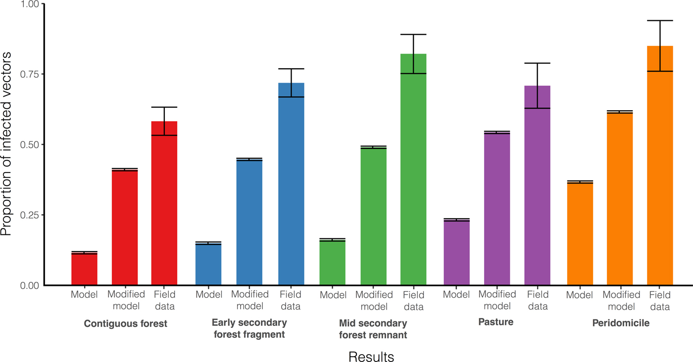
Fig. 6. Infected vector population (I v): comparison between the model without host vertical transmission, including host vertical transmission with the highest vector transmission probabilities (β high, γ high) and field results. Results are shown for the five selected habitats, for each bars set grouped by colour, the left and middle bars correspond to model results and the bar on the right to field results (Gottdenker et al. Reference Gottdenker, Chaves, Calzada, Saldaña and Carroll2012). Host vertical transmission dynamics are represented by equations (8)–(10). The model including vertical transmission considering high probabilities of transmission in vectors better approaches field data compared with the model accounting only for oral and vectorial transmission.
However, field data showed values that are much higher compared with simulation results. While the proportion of infected vectors found in the contiguous forest is the lowest with
 $58\% \;(54 - 63\%, \;95\% \;{\rm CI})$
and in the peridomicile is the highest with
$58\% \;(54 - 63\%, \;95\% \;{\rm CI})$
and in the peridomicile is the highest with
 $85\% \;(76 - 94\%, \;95\% \;{\rm CI})$
, the model without host vertical predicted
$85\% \;(76 - 94\%, \;95\% \;{\rm CI})$
, the model without host vertical predicted
 $12\;{\rm and}\;36\% $
, respectively. The same pattern occurs in intermediately disturbed habitats. We argue that this discrepancy could point out previously unconsidered mechanisms involved in parasite transmission. In other words, the model suggests that vectorial and oral routes are not sufficient to explain the high proportion of infected vectors found in the Panama Canal. Therefore, we decided to incorporate host vertical transmission in the model. Congenital transmission, under experimental studies, impacts infection in host populations (Alkmim-Oliveira et al.
Reference Alkmim-Oliveira, Costa-Martins, Kappel, Correia, Ramirez and Lages-Silva2013) and currently, the only observation of congenital T. cruzi transmission in nature was reported in bats (Añez et al.
Reference Añez, Crisante and Soriano2009). Furthermore, in opossums (Didelphis marsupialis) it is possible that offspring may become infected from the perineal region during birth, as infectious stages of T. cruzi have been found in the anal glands (Deane et al.
Reference Deane, Lenzi and Jansen1984). When we incorporate vertical transmission in hosts accompanied by an increase in the probability of infection from the infected host populations (I
h and C
h) to the susceptible vector population (I
v), our results are more similar to the empirical data from the Panama Canal (Fig. 6) than when we do not include this mechanism in the model.
$12\;{\rm and}\;36\% $
, respectively. The same pattern occurs in intermediately disturbed habitats. We argue that this discrepancy could point out previously unconsidered mechanisms involved in parasite transmission. In other words, the model suggests that vectorial and oral routes are not sufficient to explain the high proportion of infected vectors found in the Panama Canal. Therefore, we decided to incorporate host vertical transmission in the model. Congenital transmission, under experimental studies, impacts infection in host populations (Alkmim-Oliveira et al.
Reference Alkmim-Oliveira, Costa-Martins, Kappel, Correia, Ramirez and Lages-Silva2013) and currently, the only observation of congenital T. cruzi transmission in nature was reported in bats (Añez et al.
Reference Añez, Crisante and Soriano2009). Furthermore, in opossums (Didelphis marsupialis) it is possible that offspring may become infected from the perineal region during birth, as infectious stages of T. cruzi have been found in the anal glands (Deane et al.
Reference Deane, Lenzi and Jansen1984). When we incorporate vertical transmission in hosts accompanied by an increase in the probability of infection from the infected host populations (I
h and C
h) to the susceptible vector population (I
v), our results are more similar to the empirical data from the Panama Canal (Fig. 6) than when we do not include this mechanism in the model.
Another T. cruzi transmission mechanism that we do not simulate here, but could be important, is vector direct transmission. Previous laboratory studies have reported ‘kleptohemodeipnonism’ or the act of stealing blood, as a means of infection between triatomines (Ryckman, Reference Ryckman1951; Marinkelle, Reference Marinkelle1965; Añez, Reference Añez1982; Schaub, Reference Schaub1988). In addition, Gottdenker et al. (Reference Gottdenker, Chaves, Calzada, Saldaña and Carroll2012) reported nymphs collected from palms that contain blood from domestic animals, suggesting that they may have fed from engorged adults who fed on these terrestrial mammals and then returned to the palm (Gottdenker et al. Reference Gottdenker, Chaves, Calzada, Saldaña and Carroll2012). To the authors’ knowledge, there are no reported observations of this process in the wild, as it can be very difficult to observe wild vector behaviour ‘in situ’ and requires further research.
Although useful, our modelling approach has some limitations. The first limitation is considering the whole set of different host species in a particular habitat as an average ensemble of host populations. An alternative approach to study host community composition could be to model each host population independently; however, the lack of data on host species parameters related to T. cruzi transmission makes this a highly hypothetical approach. Another limitation is that the assumption of host species ingesting 1–2 vectors per week on average ignores that predation is opportunistic and many other insects besides vectors might be available to hosts (Kribs-Zaleta, Reference Kribs-Zaleta2010). Another model limitation relies in using Rhodnius neglectus intrinsic rate instead of R. pallescens. Both species belong to the same genus, but different clade (Monteiro et al. Reference Monteiro, Wesson, Dotson, Schofield and Beard2000); suggesting potential discrepancies in their life cycles. In addition, the model does not include spatial aspects of disease transmission, which may differ between discrete locations impacting the proportion of infected vectors. For instance, palm trees, the primary habitat of R. pallescens (De Vasquez et al. Reference De Vasquez, Samudio, Saldaña, Paz and Calzada2004) and most of Rhodnius species (Abad-Franch et al. Reference Abad-Franch, Lima, Sarquis, Gurgel-Gonçalves, Sánchez-Martín, Calzada, Saldaña, Monteiro, Palomeque, Santos, Angulo, Esteban, Dias, Diotaiuti, Bar and Gottdenker2015), could vary on their physiognomy, shaping bug population density and age distribution (Urbano et al. Reference Urbano, Poveda and Molina2015). In addition, palm spatial location could determine triatomine blood meals affecting epidemiological indices (Suarez-Davalos et al. Reference Suarez-Davalos, Dangles, Villacis and Grijalva2010). Thus, in an endemic area, certain palm trees might play an important role as spatial ‘source’ foci where enhanced transmission could be taking place. The preceding considerations are even more relevant if one acknowledges the importance of host predation on vectors based on the results of the sensitivity analysis.
Finally, infected host populations could be studied using the model; however, for the Panama Canal area we were not able to contrast our results to field data yet. Comparing our results with an experimental study conducted in a protected and a disturbed area in the Argentine Chaco, the model supports that T. cruzi infection within host species is significantly higher in disturbed habitats (Orozco et al. Reference Orozco, Enriquez, Cardinal, Piccinali and Gürtler2016). A similar pattern was also reported for an Atlantic Rain Forest landscape in Brazil, where patch size was studied as a means of habitat fragmentation and smaller patches showed higher T. cruzi prevalence in small mammals as compared with larger patches (Vaz et al. Reference Vaz, D'Andrea and Jansen2007). Additionally, the range values for the infected host population (2–27%) found with the models are comparable with the results reported by both studies, which were 5·7–22% (Orozco et al. Reference Orozco, Enriquez, Cardinal, Piccinali and Gürtler2016) and 6–25% (Vaz et al. Reference Vaz, D'Andrea and Jansen2007). We suggest that conducting more detailed field studies, including extensive sampling of mammal hosts potentially involved in T. cruzi transmission in habitats varying in the levels of disturbance, will help clarify the dynamics of transmission in anthropogenically altered habitats.
SUPPLEMENTARY MATERIAL
The supplementary material for this article can be found at https://doi.org/10.1017/S0031182017001287
ACKNOWLEDGEMENTS
We thank Tim Kailing, undergraduate advisor of CC, and John Drake of the NSF REU Population Biology of Infectious Disease program for feedback on earlier versions of this model.
FINANCIAL SUPPORT
D.E. and J.C. were supported by the Vice-President for research at Universidad de los Andes and Colciencias call 617. C.C. was supported by an NSF REU #1156707, ‘Population Biology of Infectious Diseases’ Research Experience for Undergraduates (REU) grant. N.G., A.S. and J.E.C. were funded by a SENACYT (La Secretaría Nacional de Ciencia, Tecnología e Innovación) grant Col Col 011-43. N.G. also received financial support from the Office of the Vice President for Research at the University of Georgia. Any opinions, findings and conclusions or recommendations expressed in this material are those of the authors and do not necessarily reflect the views of the National Science Foundation, Colciencias, University of Georgia OVPR, Universidad de los Andes and the Gorgas Memorial Institute.


