


Introduction
Microbial mats, visibly conspicuous biofilms covering the surfaces of terrestrial and aquatic sediments and cobbles, are common in physically and chemically stressed environments, and may account for the majority of biomass in polar freshwaters (Vincent & Howard-Williams Reference Vincent and Howard-Williams1986, Hawes & Howard-Williams Reference Hawes and Howard-Williams1998). These communities have high levels of endemism (Vyverman et al. Reference Vyverman, Verleyen, Wilmotte, Hodgson, Willems, Peeters, van de Vijver, de Wever, Leliaert and Sabbe2010) and are primarily composed of filamentous cyanobacteria from genera Oscillatoria Vaucher ex Gomont, Leptolyngbya Anagnostidis & Komárek, Wilmottia Strunecký, Elster & Komárek and Microcoleus Desmaziéres ex Gomont (Alger et al. Reference Alger, McKnight, Spaulding, Tate, Shupe, Welch, Edwards, Andrews and House1997), along with aerophilic diatoms that live at lower densities (Esposito et al. Reference Esposito, Spaulding, McKnight, de Vijver, Kopalová, Lubinski, Hall and Whittaker2008). Benthic mats are abundant in the thalweg of streams (Alger et al. Reference Alger, McKnight, Spaulding, Tate, Shupe, Welch, Edwards, Andrews and House1997). The mats are vertically stratified with high concentrations of chlorophyll a (chl a) in lower layers and have high concentrations of accessory pigments in upper layers, producing a vivid coloration which may be an adaptation to reduce the harmful effects of radiation (Bonilla et al. Reference Bonilla, Rautio and Vincent2009).
Mats flourish in the McMurdo Dry Valleys (MDV) of Antarctica and persist as a freeze-dried crust during winter months. Stream flow is produced from glacial melt during the 4–10 weeks of summer (McKnight et al. Reference McKnight, Niyogi, Alger, Bomblies, Conovitz and Tate1999) and mats are reactivated within as little as 20 minutes after rehydration (Vincent & Howard-Williams Reference Vincent and Howard-Williams1986). Once activated, mats may cover a large portion of the stream bed (Alger et al. Reference Alger, McKnight, Spaulding, Tate, Shupe, Welch, Edwards, Andrews and House1997) and are hotspots for biogeochemical cycling (Gooseff et al. Reference Gooseff, McKnight, Runkel and Duff2004). The MDV streams have negligible grazing activity (Treonis et al. Reference Treonis, Wall and Virginia1999), minimal lateral inputs of water and allochthonous organic material (Gooseff et al. Reference Gooseff, McKnight, Doran, Fountain and Lyons2011), and experience relatively uniform diel radiation in summer due to 24 hour sunlight. Collectively, this lack of convoluting factors makes MDV streams an ideal location to study how microbial mats interact with their physical environment.
Stream flow is variable in magnitude over the course of a summer. In MDV streams, the hydrograph predictably peaks on a diel cycle which may elevate discharge by orders of magnitude (Cullis et al. Reference Cullis, Stanish and McKnight2014). Interannual variability is also significant and the low discharges of the 1990s were associated with a cool period in the MDV (Doran et al. Reference Doran, Priscu, Lyons, Walsh, Fountain, McKnight, Moorhead, Virginia, Wall, Clow, Fritsen, McKay and Parsons2002). This trend was interrupted in 2001–02 with a high discharge ‘flood’ year (Doran et al. Reference Doran, McKay, Fountain, Nylen, McKnight, Jaros and Barrett2008). Flow has remained elevated since, punctuated with several other high flow summers (Nielsen et al. Reference Nielsen, Wall, Adams, Virginia, Ball, Gooseff and McKnight2012). With higher flows, sediment loads may increase and substrata may mobilize, leading to the scour and transport of microbial mats (Howard-Williams et al. Reference Howard-Williams, Vincent, Broady and Vincent1986, Hawes & Howard-Williams Reference Hawes and Howard-Williams1998). The McMurdo Dry Valleys Long-Term Ecological Research (MCM LTER) programme has monitored mats over the last two decades. The hydrologic regime has been shown to regulate mat biomass (Stanish et al. Reference Stanish, Nemergut and McKnight2011), transport (Cullis et al. Reference Cullis, Stanish and McKnight2014) and species composition (Stanish et al. Reference Stanish, Nemergut and McKnight2011, Reference Stanish, Kohler, Esposito, Simmons, Nielsen, Wall, Nemergut and McKnight2012). However, for these communities, the effects of discrete disturbances have not been explicitly tested as for other desert streams (e.g. Fisher et al. Reference Fisher, Gray, Grimm and Busch1982, Davie et al. Reference Davie, Mitrovic and Lim2012).
Although protected in various ways, the MDV are nonetheless projected to be both indirectly and directly influenced by human activity in the coming decades. As the ozone hole ameliorates, Continental Antarctica is projected to warm (Walsh Reference Walsh2009), aligning with trends already observed on the Antarctic Peninsula (Richard et al. Reference Richard, Rouault, Pohl, Crétat, Duclot, Taboulot, Reason, Macron and Buiron2013). Stream flow may increase from greater glacial melt and high flow summers could create disturbances by providing ‘pulse events’ (Nielsen et al. Reference Nielsen, Wall, Adams, Virginia, Ball, Gooseff and McKnight2012). There may also be increased physical disturbances associated with direct anthropogenic activity in MDV due to increased numbers of visitors. Because of the slow estimated growth rates (Vincent & Howard-Williams Reference Vincent and Howard-Williams1986), mats could be susceptible to human disturbance such as trampling, although the known or potential human impacts are limited and have not been measured despite 60 years of research in the MDV.
In this study, two questions were addressed: i) how does microbial mat biomass recover from a scouring disturbance over different flow seasons? ii) Do these events have observable effects on elemental composition and algal community structure? Microbial mat recovery from simulated disturbance treatments was monitored to understand the impact that physical disturbances have on the colonization, structure and subsequent development of algal communities in these habitats. The results of this study may be used to help interpret long-term trends, explain spatial differences in elemental composition and guide policy for Antarctic Specially Managed/Protected Areas (ASMAs and ASPAs, www.mcmurdodryvalleys.aq) and organizations such as the International Association of Antarctic Tour Operators (IAATO, www.iaato.org).
Methods
Site description
The MDV are the largest ice free area in Antarctica (~4800 km2) and are located along the coast of McMurdo Sound in south Victoria Land. Because of the unique nature of this region, the MDV are managed within an ASMA intended to minimize conflicting uses and help to protect sensitive geological and biological features. During the continual sunlight of summer months (November to January) air temperatures range from -10 to 5°C, and meltwater from alpine, piedmont and terminal glaciers form streams that flow into permanently ice-covered, closed-basin lakes on the valley floors. The MDV are extremely arid and receive <50 mm water equivalent annually as snowfall, which primarily sublimates (reviewed by Gooseff et al. Reference Gooseff, McKnight, Doran, Fountain and Lyons2011). Stream solute concentrations reflect weathering reactions in the hyporheic zone and biogeochemical processes occurring in the cyanobacterial mats (Gooseff et al. Reference Gooseff, McKnight, Runkel and Duff2004).
Green Creek (-77.624108, 163.060101) is located in Taylor Valley, ~12 km from the coast and ~1.2 km in length with a shallow gradient and an intermediate sized cobble pavement substratum (Fig. 1). Cyanobacterial mats grow throughout its length, generating some of the highest levels of biomass reported in the MDV (Alger et al. Reference Alger, McKnight, Spaulding, Tate, Shupe, Welch, Edwards, Andrews and House1997). Green Creek drains a glacial melt pond, thus seasonal variability in flow regime is lower than in other dry valley streams that may experience abrupt termination in flow following cooling temperatures, such as on cloudy days. This stream was chosen as the study site because the Taylor Valley Visitor Zone is located near its headwaters, the only tourist destination for cruise ship helicopter passengers in MDV (O’Neill et al. Reference O’Neill, Balks and López-Martínez2013), and it has also been the site of several experiments (i.e. Gooseff et al. Reference Gooseff, McKnight, Runkel and Duff2004, Stanish et al. Reference Stanish, Nemergut and McKnight2011). Furthermore, Green Creek discharge, biology and chemistry has been monitored by the MCM LTER programme since 1993–94 using field and analytical methods described in Stanish et al. (Reference Stanish, Nemergut and McKnight2011). As a result, chemical and biological components of Green Creek are comparatively well studied.
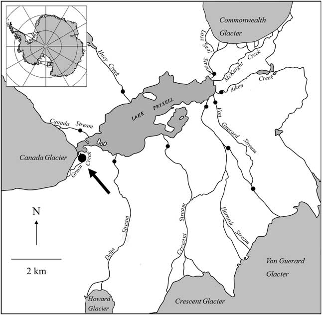
Fig. 1 Detail of the Lake Fryxell basin within Taylor Valley, Antarctica. The black circles indicate gaging stations operated by the MCM LTER, and the black arrow points to the Green Creek study site.
Experimental design
To test how mats recolonize substrata over time, the regrowth of cyanobacterial mats was characterized on rocks taken upstream of the MCM LTER algal transect and downstream of the Taylor Valley Visitor Zone over two summers. These locations were chosen for mat epilithon sampling because these rock communities are potentially trampled by human foot-traffic crossing the stream. The first regrowth experiment took place during the 2001–02 summer, which coincidentally was the highest flow season on record (Doran et al. Reference Doran, McKay, Fountain, Nylen, McKnight, Jaros and Barrett2008). A second experiment took place over the 2012–13 summer, which had flows that were lower in magnitude. In both seasons, epilithic mat material was collected ~1 week after the onset of stream flow, allowing microbial communities to reactivate from the dormant state before the first sampling period.
In both experiments, 30 rocks were removed from the stream bed early in the season (day 0, 13 December 2001 and 12 December 2012), taking care not to disturb untreated substrata. While rocks were mostly selected without bias, those that were big enough to accumulate measureable growth after several weeks but not so large that removal would affect the stream morphology were chosen (average exposed rock area ~118 cm2). Substrata were uniformly covered by a thick (~0.5 cm) orange mat. The mat material on top of each rock was removed with a toothbrush and rinsed into a container with stream water. The resulting slurry was transferred to a bottle or Whirlpack® bag and kept chilled and away from light until processed in the laboratory within 24 hours. The rocks were numbered, fitted with aluminium foil to measure surface area, returned to the same location in the stream and marked with surveying flags.
For 2001–02, the same rocks were resampled to measure regrowth at the end of the summer as flow began to slow (day 43, 25 January 2002), utilizing the same methods described above. Samples were not taken midway through the 2001–02 summer due to logistical problems associated with the high consistent flow. For 2012–13, half of the previously sampled rocks were resampled on day 22 (3 January 2013, n=15) and the other half on day 38 (19 January 2013, n=15). On each of these days an additional 15 rocks that had not been previously manipulated were sampled. These previously unsampled rocks were taken from the immediate vicinity of the resampled rocks and served as a control to measure background growth.
In 2001–02, all mat samples were filtered onto precombusted, preweighed Whatman® GF/F glass fibre filters and were immediately frozen and stored until analysis. Fifteen samples were analysed for ash-free dry mass (AFDM). The other 15 samples were cut in half and analysed for chl a or other elemental (carbon:nitrogen:phosphorus) content (final n=14 for both chl a and stoichiometry). In 2012–13, each rock sample was split quantitatively into four aliquots for chl a, AFDM, stoichiometry and algal community composition by homogenizing the entire sample and splitting by volume. The AFDM and chl a aliquots were filtered onto ashed, preweighed Whatman® GF/F filters and immediately frozen until analysis. The algal community aliquot was promptly preserved in ~5% formalin solution and shipped to the University of Colorado, at room temperature.
Biomass
For 2001–02, chl a was analysed by grinding and extracting the filters in 90% buffered acetone, centrifuging the extracts and analysing the supernatant using the trichromatic method (Strickland & Parson Reference Strickland and Parsons1972). For 2012–13, chl a was measured by extracting samples in 90% buffered acetone for 24 hours and analysed on a Turner 10-AU Fluorometer (Welschmeyer Reference Welschmeyer1994). The AFDM was determined by drying samples at 55°C until a constant dry mass was achieved, ashing filters at 450°C for 4 hours and rewetting (Steinman et al. Reference Steinman, Lamberti and Leavitt1996). Resulting AFDM and chl a estimates were scaled to the surface area of the rock of origin, which was calculated by applying a regression of known foils weights to known foil area (Steinman et al. Reference Steinman, Lamberti and Leavitt1996). An autotrophic index (AI) was calculated by dividing chl a values with corresponding AFDM. Percent organic material was calculated by dividing AFDM by the total sample mass. All biomass analyses were performed in Crary Laboratory at McMurdo Station.
Stoichiometry
The C:N:P aliquots were dried in an oven at 50–55°C, homogenized and ground to a fine powder. The %C and %N was measured using a Carlo Erba 1500 Elemental Analyzer (CE Instruments, Wigan) for 2001–02 samples, and a FlashEA® 1112 Organic Elemental Analyzer (Thermo Finnigan, Milan) for 2012–13 samples. The %P aliquot was ashed in a muffle furnace at 500°C for 1 hour, digested with 1N HCl and analysed as orthophosphate, with samples from 2001–02 estimated by the procedure of Smeller (Reference Smeller1995) by Optical Emission Spectroscopy (Specto) and 2012–13 on a Lachat QuikChem 8500 Flow Injection Analyzer (Hach Company, Loveland, CO) by the Kiowa Laboratory at the University of Colorado (Boulder, CO; Murphy & Riley Reference Murphy and Riley1962). The resulting values were then converted to molar C:N, C:P and N:P ratios.
Community characterization
To investigate if simulated disturbance treatments had an effect on community structure, epilithic mat communities were characterized morphologically by light microscopy for the 2012–13 summer samples utilizing methods similar to Alger et al. (Reference Alger, McKnight, Spaulding, Tate, Shupe, Welch, Edwards, Andrews and House1997). Briefly, five samples for each treatment and date (ten for day 0, 30 in total) were randomly chosen, homogenized and a ~1 ml aliquot was transferred into a concave microscope slide and observed under 400x magnification. Each filament, colony or solitary cell was classified as one natural unit and identified to the lowest taxonomic designation possible (generally genus), and at least 150 units were counted for each sample. Diatoms were always counted as one unit, even if forming a colony, and the viability of each frustule (live or dead) was documented. Live diatoms were classified as those that had protoplast material remaining in the frustule at the time of preservation. After enumeration of the community was complete, the slide was scanned for several minutes for more diatoms (to increase live/dead sample size) and the percentage of live and dead diatoms encountered was then calculated.
Representative soft algal cells (in a colony, filament or solitary) were counted and measured in each field with the ocular micrometre. Dimensions for diatoms were measured if possible, but if a valve was obstructed making measurement impossible, width and length averages were taken from the Antarctic Freshwater Diatoms website (http://huey.colorado.edu/diatoms/about/index.php). Valve depth was estimated for genera as follows, based on measurements during the study: 12.5 µm for Hantzschia, 10 µm for Muelleria, 5 µm for Luticola, 3.75 µm for Stauroneis and 2.5 µm for all others. Relative biovolumes of the taxonomic groups were then calculated using equations from Hillebrand et al. (Reference Hillebrand, Dürselen, Kirschtel, Pollingher and Zohary1999). Komárek & Anagnostidis (Reference Komárek and Anagnostidis2005) was the primary resource used for cyanobacterial identification. Although the Phormidium spp. in our samples have recently been transferred to the genus Microcoleus (Strunecký et al. Reference Strunecký, Komárek, Johansen, Lukešová and Elster2013); single trichomes are referred to classically as ‘Phormidium’ and multiple trichomes in a sheath as ‘Microcoleus’ to avoid confusion.
Diatoms were further described to species by digesting another aliquot from the corresponding samples in 30% H2O2 with low heat and rinsed with distilled water until a neutral pH was achieved. The digested material was dried onto cover slips and mounted onto glass microscope slides with the mounting medium Zrax® (refractive index=1.7; W.P. Dailey, University of Pennsylvania, Philadelphia, PA). Relative abundances of diatom species were determined using an Olympus Vanox light microscope (Japan) at 1250× magnification, with ≥300 valves enumerated per slide. Diatoms were identified to species according to descriptions from Esposito et al. (Reference Esposito, Spaulding, McKnight, de Vijver, Kopalová, Lubinski, Hall and Whittaker2008), Kopalová et al. (Reference Kopalová, Veselá, Elster, Nedbalová, Komárek and van de Vijver2012) and the Antarctic Freshwater Diatoms website.
Flow and water chemistry
Green Creek stream flow and water temperature are continuously monitored at the outlet to the lake, and discharge was measured as part of the MCM LTER with the use of a pressure transducer logging at 15 minute intervals. Stream water was collected concurrently with each site visit throughout both summers. All water chemistry sampling and analyses were conducted following the methods outlined in Welch et al. (Reference Welch, Lyons, Whisner, Gardner, Gooseff, McKnight and Priscu2010). Briefly, raw water was collected in triple-rinsed 250 ml Nalgene® bottles for nutrient samples and 125 ml precombusted amber glass bottles for dissolved organic carbon (DOC). Water for nutrient analysis was filtered from the raw water sample on glass fibre filters and frozen for later analysis at the field station. Cation and anion samples were filtered with Nuclepore™ polycarbonate membrane filters with 0.4 mm pore size and refrigerated at 4°C. Samples for DOC were filtered and acidified using concentrated HCl and stored at 4°C for later analysis at the Crary Laboratory at McMurdo Station. All discharge and chemistry data are available at http://www.mcmlter.org.
Statistical analyses
All variables that were not normally distributed were log-transformed to satisfy the assumption of normality. Pairwise t-tests were conducted to directly compare rock variables at initial and final time points (before and after disturbance). To test if disturbed rock variables were significantly different from controls on the same dates, or if initial or final rock variables were different between the two flow seasons (i.e. comparisons between different sample pools), means were compared with a Welch two sample t-test. Thirty rocks were scraped on day 0 in 2012–13, whereas 15 were sampled for regrowth and controls respectively on day 22 and 38, as well as both sample dates in 2001–02. To avoid differences in the number of observations, the regrowth on individual rocks from day 0 were directly compared with later dates from 2012–13. The rocks sampled for regrowth on day 22 are ‘group A’ and rocks resampled on day 38 are ‘group B’. When final and initial values between the 2001–02 and 2012–13 summers were compared, only rock data from day 0 that corresponded with the rock regrowth on day 38 were used (group B).
For community data, non-Euclidean Redundancy Analyses (RDA) were created to visualize differences between algal and diatom communities between treatments and days utilizing the vegan R package. Rare species that occurred <5.0% by relative abundance or biovolume were removed and data were square root transformed to satisfy assumptions of normality. An extra diatom community sample was counted for a regrown mat on day 38, and was included in the multivariate analysis but not the direct comparisons of relative abundances as outlined above for biomass and stoichiometry. Significance of sample day and treatment were evaluated by permutational multivariate analysis of variance (PERMANOVA), significance at α=0.05. Additionally, identical analyses were performed for diatom communities, excluding Fistulifera pelliculosa (Brébisson ex Kützing) Lange-Bertalot whose origin and ecology are ambiguous (Stanish et al. Reference Stanish, Kohler, Esposito, Simmons, Nielsen, Wall, Nemergut and McKnight2012).
All statistical analyses were performed using the R statistical environment, version 2.13.0 (R Core Team 2014).
Results
Discharge, mats and nutrients
The summer of 2001–02, regarded as the ‘flood year’, is the highest flow season in Green Creek on record (Fig. 2a, Doran et al. Reference Doran, McKay, Fountain, Nylen, McKnight, Jaros and Barrett2008). There were consistent high discharges throughout the year (Fig. 2b). The average flow was 72 l s-1 and the maximum flow recorded was 315 l s-1. The total discharge was 3.41x10⁸ l. Nutrient concentrations for 2001–02 summer averaged 10.48 µg N-NO3 - l-1, 2.16 µg N-NO2 - l-1, 4.81 µg N-NH4 + l-1 and 4.40 µg P-soluble reactive phosphorus (SRP) l-1 (Table I).
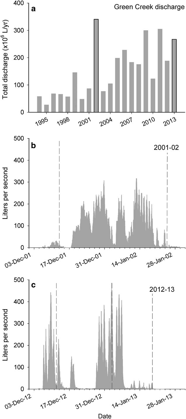
Fig. 2 a. Total calculated discharge taken from the Green Creek gage (F9) for each summer for 1993–94 through 2012–13. Darkened bars indicate summers highlighted in this study. b. & c. Hydrograph of the continuous discharge measurements taken from the Green Creek stream gage (F9) during the 2001–02 and 2012–13 summers, respectively. Dotted lines indicate dates epilithon was sampled.
Table I Values for physical and chemical parameters opportunistically sampled from Green Creek stream water during the 2001–02 and 2012–13 summers.
DOC=dissolved organic carbon, NA=not applicable, SC=specific conductance, SRP=soluble reactive phosphorus.
Flows for 2012–13 were more intermittent compared to 2001–02, and the stream experienced prolonged periods without flow, though at discrete intervals exhibited punctuated high flow events (Fig. 2c). The average discharge for 2012–13 summer was 61 l s-1 and the maximum flow recorded was 485 l s-1. Despite the intermittent nature, high flows brought the total discharge to 2.67x10⁸ l, which is the third highest total discharge for this stream since the 1993–94 summer. Nutrient concentrations averaged 15.87 µg N-NO3 - l-1, 1.31 µg N-NO2 - l-1, <5 µg N-NH4 + l-1 (detection limit) and 3.85 µg P-SRP l-1 (Table I).
Over the last two decades of microbial mat monitoring in Green Creek, orange mat biomass from the downstream algal transect has been higher on average than epilithon measured in this study, ranging from 1.07 to 11.16 µg cm-2 for chl a (Fig. 3a) and 3.08 to 16.99 mg cm-2 for AFDM (Fig. 3b). For the 2012–13 summer, orange mat biomass averaged 4.29 µg chl a cm-2 and 6.40 mg AFDM cm-2. Similarly, 2011–12 biomass averaged 7.24 µg chl a cm-2 and 7.43 mg AFDM cm-2. Average nutrient ratios for orange mats measured in this year were C:N=9.55, C:P=74.34 and N:P=7.77. Mat samples were not taken during the 2001–02 summer due to challenges associated with sustained high flows, but averaged 9.73 µg chl a cm-2 and 10.02 mg AFDM cm-2 in 2000–01, and 7.28 µg chl a cm-2 and 3.12 mg AFDM cm-2 in 2002–03 (Fig. 3a & b).
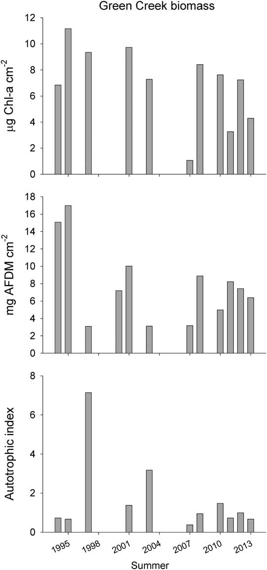
Fig. 3 Average a. chl a, b. ash-free dry mass (AFDM) and c. autotrophic index (AI=chl a:AFDM) for monitored orange mats sampled at the downstream Green Creek transect as part of the MCM LTER for each summer, 1993–94 through 2012–13. Where bars are absent samples were not taken. See Stanish et al. (Reference Stanish, Nemergut and McKnight2011) for detailed collection and analytical methods.
Comparison of mat recovery between two summers
Mat biomass measured as epilithon was substantially less than the thick mats monitored as part of the MCM LTER. Initial chl a measurements averaged 1.18 µg chl a cm-2 for 2001–02 and 1.00 µg chl a cm-2 for 2012–13, and were not statistically different (Fig. 4a). The final chl a concentrations were significantly lower in 2012–13 (Welch’s t-test, t=4.49, df=26.94, P<0.01), and averaged 0.18 µg cm-2 in 2012–13 compared to 0.56 µg cm-2 in 2001–02 (Fig. 4a). Final rock samples had significantly less chl a than initial samples in 2001–02 (Paired t-test, t=4.19, df=12, P<0.01) and 2012–13 (Paired t-test, t=-5.49, df=14, P<0.01). The AFDM was not significantly different at the beginning of the two seasons and averaged 1.50 and 1.15 mg AFDM cm-2 for 2001–02 and 2012–13, respectively (Fig. 4b). The AFDM values were lower at the end of 2012–13, averaging 0.31 mg cm-2 compared to 0.61 mg cm-2 for 2001–02 (Welch’s t-test, t=2.61, df=19.99, P=0.02). Lastly, mat AFDM was significantly reduced from the initial to the final sampling in both 2001–02 (Paired t-test, t=4.01, df=14, P<0.01) and 2012–13 (Paired t-test, t=-5.92, df=14, P<0.01). The percent regrowth was greater in 2001–02 compared to 2012–13 for chl a (47% and 18%) and AFDM (40% and 27%).
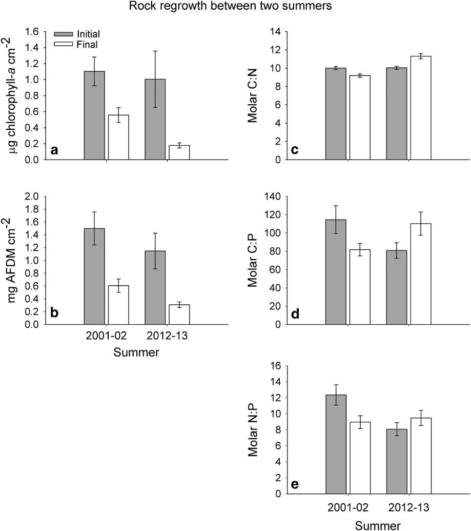
Fig. 4 Recovery of epilithic biomass (a. chl a and b. ash-free dry mass (AFDM)) and stoichiometry (c. C:N, d. C:P and e. N:P) from rock samples measured at the beginning and end of the 2001–02 and 2012–13 summers. Error bars indicate standard error.
Initial C:N ratios of mats averaged 10.02 and 10.04 for 2001–02 and 2012–13, respectively, and were not statistically different (Fig. 4c). However, the final ratios in 2012–13 were significantly greater than the final ratios in 2001–02, averaging 9.19 and 11.45, respectively (Welch’s t-test, t=-7.23, df=23.68, P<0.01). Within seasons, initial mats had greater C:N ratios than final samples in 2001–02 (Paired t-test, t=3.75, df=12, P<0.01), and final mats had greater C:N ratios than initial in 2012–13 (Paired t-test, t=5.04, df=13, P<0.01, Fig. 4c). In contrast, C:P ratios were only marginally greater for 2001–02 initial material, averaging 114.50 versus 80.92 for 2012–13 (Welch’s t-test, t=1.93, df=20.53, P=0.07, Fig. 4d). Final C:P ratios were marginally greater in 2012–13 than 2001–02 (Welch’s t-test, t=-1.98, df=19.87, P=0.06). Within summers, initial C:P ratios were greater than final in 2001–02 (Paired t-test, t=3.17, df=13, P=0.01), but in 2012–13 final ratios were significantly greater than initial (Paired t-test, t=4.27, df=13, P<0.01, Fig. 4d). These patterns were the same for N:P ratios, though less pronounced (Fig. 4e). The N:P ratios were significantly greater in the initial mats from 2001–02 compared to 2012–13 (Welch’s t-test, t=2.82, df=22.35, P=0.01), but there was no significant difference between the 2001–02 and 2012–13 final mats (Fig. 4e). Mat N:P was significantly greater in initial mats than resampled mats in 2001–02 (Paired t-test, t=3.81, df=13, P<0.01), but significantly greater in resampled mats in 2012–13 compared to initial mats (Paired t-test, t=2.72, df=13, P=0.02, Fig. 4e).
Biomass and stoichiometry over the 2012–13 summer
The differences between group A and group B on day 0 were not significant for any variable. Chlorophyll a was greatest in the middle of the growing season (day 22), with the control samples averaging 1.53 µg chl a cm-2 (Fig. 5a). Experimentally scoured rocks had significantly lower chl a concentrations than control rocks on day 22 (Welch’s t-test, t=13.10, df=25.05, P<0.01) and day 38 (Welch’s t-test, t=8.33, df=24.77, P<0.01), and averaged 0.09 µg chl a cm-2 on day 22 and 0.18 µg chl a cm-2 on day 38 (Fig. 5a). Compared to initial values, 11% of the chl a was regrown by day 22 and 18% by day 38. Averaged values for AFDM increased throughout the sampling period in the control mats and ranged from 1.15 (primary group B) to 1.60 (control 2, Fig. 5b). Again, cleaned rocks had significantly less AFDM than control rocks on day 22 (Welch’s t-test, t=-9.43, df=14.22, P<0.01) and day 38 (Welch’s t-test, t=-5.10, df=14.86, P<0.01). Mats that were cleaned of mat material on day 0 regrew 12% of their biomass compared to the initial values by day 22 and 27% of initial biomass by day 38, averaging 0.16 and 0.31 mg AFDM cm-2, respectively (Fig. 5b).
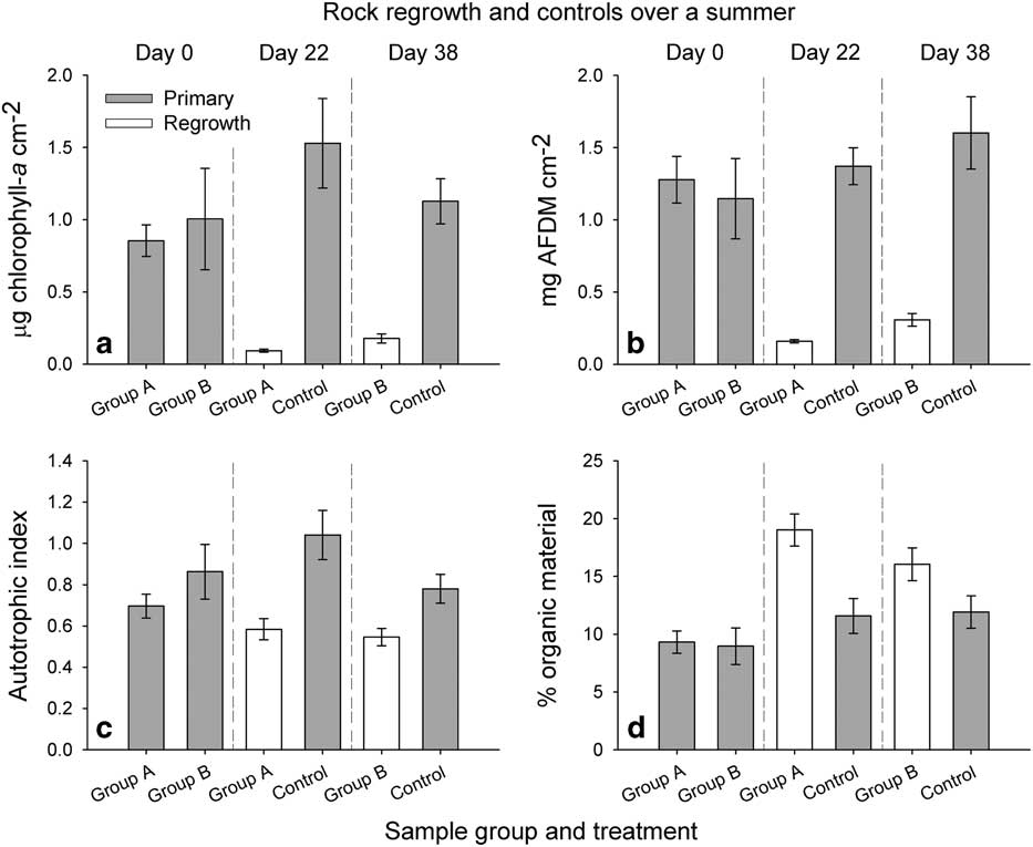
Fig. 5 Biomass as a. chl a, b. ash-free dry mass (AFDM), c. autotrophic index (AI=chl a:AFDM) and d. the percent organic material for each group of rocks and associated controls for the 2012–13 summer. Grey bars indicate the primary samples and white bars indicate regrowth. Samples are arranged by date. Error bars indicate standard error.
As for chl a, the AI was greatest on day 22 for undisturbed mats (Fig. 5c). Experimentally scoured rocks had significantly lower AI values than controls on day 22 (Welch’s t-test, t=-4.27, df=26.90, P<0.01) and day 38 (Welch’s t-test, t=2.86, df=22.99, P=0.01, Fig. 5c). The average percent organic content for undisturbed samples increased throughout the growing season, ranging from 9.0% (primary group B) to 11.9% (control 2; Fig. 5d). However, cleaned rocks had a greater percent organic content, with the greatest values measured on day 22 (19.0%), decreasing by day 38 (16.1%). Organic content at day 22 was significantly greater than all background samples (Fig. 5d). At day 38, percent organic content was only significantly greater than the primary mats from day 0 (Fig. 5d).
The %C, %N and %P were greatest in the regrowth from group A on day 22 (Fig. 6a–c). However, the nutrient content of resampled rocks was not significantly different from controls on day 22 or day 38. Molar C:N ratios of all samples were above the Redfield ratio of ~7, and increased throughout the summer, ranging from 10.0 on day 0 (both group A and B) to 11.8 on day 38 (control 2, Fig. 6d). Material from regrowth had significantly greater C:N ratios than control samples on day 22 (Welch’s t-test, t=2.26, df=27.20, P=0.03) but not on day 38 (Fig. 6d). Molar C:P ratios were approximately at or above the Redfield ratio of ~106, and ranged from 105 on day 38 (control 2) to 125 on day 22 (group A), but regrowth was not significantly different from controls on either sample date (Fig. 6e). For molar N:P ratios, all values were below the Redfield ratio of 16, and ranged from 8.1 (primary group B) to 11.2 (control 1, Fig. 6f). Similar to C:P, average N:P values were greatest on day 22, but regrowth was not significantly different than controls on either day 22 or 38 (Fig. 6f).
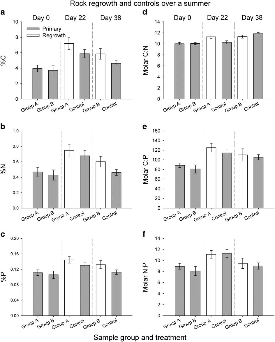
Fig. 6 Nutrient composition of epilithon for each group of rocks and associated controls for the 2012–13 summer: a. %C, b. %N and c. %P, and e. C:N, f. C:P and g. N:P. Grey bars indicate the primary samples and white bars indicate regrowth. Samples are arranged by date. Error bars indicate standard error.
Microbial community structure
Epilithic communities were dominated by genera Nostoc Vaucher ex Bornet & Flahault, Phormidium (solitary Microcoleus), Oscillatoria and Wilmottia (Fig. 7a). Minor genera (compiled in ‘other’ category) included representatives from Calothrix C.Agardh ex Bornet & Flahault, Leptolyngbya, Microcoleus (colonial), Nodularia Mertens ex Bornet & Flahault, Pseudoanabaena Lauterborn and Schizothrix Kützing ex Gomont. The disturbance treatment had visible effects on community structure, with the proportion of Oscillatoria spp. being greater on substrata that had been disturbed (mean±standard error, 45.2%±5.8 vs 31.6%±3.3) and Phormidium spp. more scarce in biovolume on disturbed substrata (11.0%±2.8 vs 36.4%±4.3).
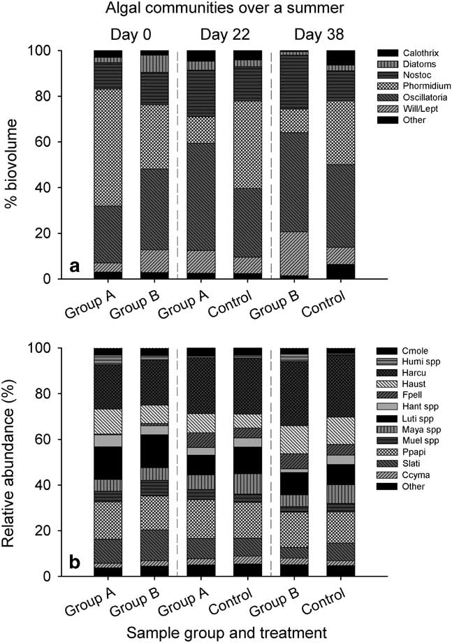
Fig. 7 a. Overall epilithic community by percent biovolume and b. relative abundance of major groups of diatoms. For the composite figure, Wilmottia spp. and Leptolyngbya spp. are combined. Cmole=Craticula molestiformis (Hustedt) Mayama, Humi spp=Humidophila spp., Harcua=H. arcuata, Haust=H. australis, Fpell=Fistulifera pelliculosa, Hant spp=Hantzschia spp., Luti spp=Luticola spp., Maya spp=Mayamaea spp., Muel spp=Muelleria spp., Ppapi=Psammothidium papilio, Slati=Stauroneis latistauros and Ccyma=Chamaepinnularia cymatopleura (West & West) Cavacini.
Diatoms comprised a small proportion of the communities, 0–27% of the total biovolume, with an average of 3.4% (± 0.97). The live/dead status of diatoms was also variable throughout the flow year and by treatment. Diatoms from group A averaged 54% viable (n=43) and group B 41% (n=65) on day 0. By day 22, 29% of diatoms had intact chloroplasts in group A (n=18), as opposed to the control group with 76% (n=44). On the last sample date, group B had 47% viable diatom frustules (n=28) and the control had 40% (n=35). It is possible that diatom biovolume and viability was prejudiced by our inability to see smaller frustules, as larger cells from genera Stauroneis Ehrenberg, Luticola D.G.Mann, Hantzschia Grunow and Muelleria (Frenguelli) Frenguelli were the most commonly encountered. These were small members of the communities by relative abundance, with small frustules from genera Psammothidium L.Buhtkiyarova & Round and Humidophila Lowe, Kociolek, Johansen, Van de Vijver, Lange-Bertalot & Kopalová being the most numerous (see below).
Consistent with other studies from the continent, diatom community diversity was low in comparison with the rest of the Antarctic region, with only 35 species from 17 genera observed. Communities were largely similar throughout the experiment, although there were some notable exceptions with some taxa (Fig. 7b). Stauroneis latistauros Van de Vijver & Lange-Bertalot averaged 16% of the community on day 0, but was reduced by ~50% on subsequent days. Muelleria spp. showed the same pattern, with an average of 7% of the community belonging to the genus on day 0, decreasing by 50% in subsequent days. Fistulifera pelliculosa exhibited the opposite trend; contributing <1% of the community on day 0, and growing in relative abundance over the course of the flow season, with the greatest abundances in disturbed mat communities. Luticola spp. decreased in relative abundances over the course of the season, with less Luticola present in disturbed communities. Psammothidium papilio (D.E. Kellogg, Stuiver, T.B. Kellogg & Denton) Van de Vijver & Kopalová remained relatively constant throughout time and treatments with the exception of day 22, where they made up 17% of the communities on average. Hantzschia spp. also showed no visible change over time or treatment. Diatom communities from epilithon were very similar to those sampled from orange mats over the same season, and were dominated by Humidophila spp., P. papilio, S. latistauros and Luticola austroatlantica Van de Vijver, Kopalová, Spaulding & Esposito.
The results from permutation tests (PERMANOVA) suggest treatment (primary versus regrowth) was a highly significant factor in structuring epilithic communities (F=5.40, P<0.01). However, sample day was not a significant factor for the epilithic communities as measured by percent biovolume of cyanobacteria and diatoms (F=1.56, P=0.15). When diatom relative abundances were tested, samples were significantly different as a function of disturbance treatment (F=2.34, P=0.02), as well as the date sampled (F=2.89, P<0.01). When F. pelliculosa was removed from the dataset, sample day remained significant (F=2.07, P=0.01) but not the effect of treatment (F=1.47, P=0.13).
To investigate the drivers of this variability, epilithic communities were plotted in an RDA as a function of treatment (Fig. 8a). For the entire epilithic community, Phormidium drives most of the variation along axis 1 and 2, and is nearest to many of the primary samples, followed by Oscillatoria and Nostoc which are closer to regrowth. Calothrix explained variation in axis 2, aligning with primary samples. When diatom communities were plotted as an RDA, F. pelliculosa drives most of the treatment effects, aligning closely with the samples from regrown mats (Fig. 8b). Diatom communities further separated along both axes as a function of date sampled. RDA axis 1 explained 24.5% of the variation, and was driven by abundances of Stauroneis, Muelleria and Luticola spp. on one side, and Humidophila spp. and F. pelliculosa on the other (Fig. 9a). RDA axis 2 explained 13.4% of the variation, and driven mainly by H. arcuata (Heiden) Lowe, Kociolek, Johansen, Van de Vijver, Lange-Bertalot & Kopalová and H. australis (Van de Vijver & Sabbe) Lowe, Kociolek, Johansen, Van de Vijver, Lange-Bertalot & Kopalová on the top, with F. pelliculosa on the bottom. When F. pelliculosa was removed, these patterns remained, though day 22 and 38 samples became more similar to day 0 (Fig. 9b).
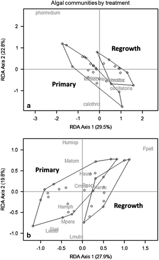
Fig. 8 Redundancy analysis (RDA) of a. composite and b. diatom communities separated by disturbance treatment. Cmole=Craticula molestiformis, Fpell=Fistulifera pelliculosa, Hamph=Hantzschia amphioxys (Ehrenberg) Grunow, Humisp=Humidophila spp., Harcua=H. arcuata, Haust=H. australis, Laustr=L. austroatlantica, Lmutic=L. muticopsis, Matom=Mayamaea atomus (Kützing) Lange-Bertalot, Mpera=Muelleria peraustralis (West & West) Spaulding & Stoermer, Ppapi=Psammothidium papilio and Slati=Stauroneis latistauros.
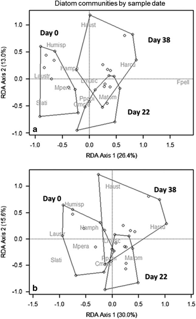
Fig. 9 Redundancy analysis (RDA) of diatom communities as a function of sample date with a. all species and b. excluding the small diatom Fistulifera pelliculosa. Abbreviations for diatom taxa are given in the caption for Fig. 8.
Discussion
Microbial mats dominate biomass in Antarctic streams, and the factors that regulate their abundance are important ecological considerations for the MDV, especially under increasing human pressures and changing environmental conditions. In this study, epilithic AFDM and chl a were substantially reduced after a scouring disturbance and regrowth rates ranged from ~20–50% over the summer. Based on these results, it follows that epilithic mats in Green Creek require multiple flow seasons without further perturbation before returning to the prior biomass (Vincent & Howard-Williams Reference Vincent and Howard-Williams1986, Hawes & Howard-Williams Reference Hawes and Howard-Williams1998), placing the MDVs on the high end of the recovery spectrum compared to mid-latitude streams (Fisher et al. Reference Fisher, Gray, Grimm and Busch1982, Davie et al. Reference Davie, Mitrovic and Lim2012). Furthermore, disturbed communities had reduced proportions of Phormidium spp. and elevated Oscillatoria spp. The effects of disturbance were less apparent for nutrient ratios and diatom community structure. Rather, there was temporal variation in the nutrient stoichiometry and diatom community structure as the growing season progressed.
Biomass
Elevated flows may stimulate in-stream mat growth through decreasing cellular boundary layers and increasing nutrient delivery (Biggs et al. Reference Biggs, Goring and Nikora1998). While mats are adapted to withstand drying, periods of low desiccating flows result in reduced productivity (Wyatt et al. Reference Wyatt, Rober, Schmidt and Davison2014). For these reasons, increases in growing season length (i.e. days with stream flow) accompanying climate warming may ultimately increase mat biomass in the MDV. However, stream microbial mats also exhibit losses due to scouring, where a threshold is met in which turbulence or sediment loads removes mat material from substrata (Hawes & Howard-Williams Reference Hawes and Howard-Williams1998). Mat biomass in several streams was previously shown to decrease after the high flow summer of 2001–02 (Stanish et al. Reference Stanish, Nemergut and McKnight2011), and the transport of mat material has been modelled as a function of diel hydrology in another Fryxell basin stream (Cullis et al. Reference Cullis, Stanish and McKnight2014).
In this study, more biomass was recovered during the summer with a higher total discharge (2001–02). This is probably because the initial set of 2001–02 samples were taken in the midst of low steady discharges and final samples were taken after some higher flows at the end of the summer. As a result, cobble substrata remained wetted for the majority of this flow season. In contrast, the initial samples in 2012–13 were taken after some potentially scouring discharges (see peaks in Fig. 2c) and the final samples were taken during a time of prolonged low flow which may have desiccated substrata outside the thalweg. It may follow that the variability of future hydrologic regimes, rather than magnitude alone, dictates whether biomass will accumulate or be reduced in MDV streams, and testing multiple hydrologic indices over a broad spatial scale will be necessary to evaluate this prediction.
Previous investigators in Maritime Antarctic streams have demonstrated variable chl a and AFDM measurements over the course of a summer (Davey Reference Davey1993, Pizarro & Vincour Reference Pizarro and Vincour2000), probably due to variability in physical and chemical characteristics over the longitudinal gradient of the stream and over the flow season. Davey (Reference Davey1993) demonstrated that spatial and temporal heterogeneity were important factors for biomass, as chl a concentrations differed by stream habitat sampled (channel or margin). In our study, day 22 stands out as having the greatest biomass during the 2012–13 summer (as well as the greatest proportion of viable diatoms), which coincided with a period of high flow. This illustrates that MDV streams are intra- as well as inter-seasonally dynamic ecosystems.
Stoichiometry
Trends between the initial and final nutrient ratios over the two summers were opposite. All stoichiometric ratios decreased from initial to final in 2001–02, while increasing over 2012–13. As for biomass, this may be due to increased nutrient delivery associated with higher (non-scouring) discharges (Biggs et al. Reference Biggs, Goring and Nikora1998). Since the first summer had more consistent flow (and terminated later), it follows that more nutrient resources were made available for uptake and assimilation. Conversely in 2012–13, where flow was regularly disrupted and ceased earlier, fewer nutrients were taken up, and those that were assimilated may have been used for maintenance rather than reproduction, especially at the end of the summer when flows were low. Similarly, the release of exudates and proteins that can occur with desiccation (Wyatt et al. Reference Wyatt, Rober, Schmidt and Davison2014) may have direct stoichiometric consequences by changing the protein to carbohydrate ratios in epilithon.
Patterns in stoichiometry may be partially explained by corresponding trends in biomass. For example, as AFDM increased throughout the 2012–13 summer, %C also increased as reflected in C:N and C:P ratios. As chl a is a nitrogen rich molecule (four N atoms each), the peak in chl a on day 22 may help explain the concurrent increase in N:P. The C:N ratios were also higher in the 2012–13 summer compared to 2001–02, the latter of which had greater chl a values. The higher initial C:P and N:P ratios in 2001–02 versus the lower final values may indicate that growing cyanobacterial mats contain more cellular P allocated for reproductive material than the established mats. Therefore, it is expected that stoichiometry, as well as biomass, has varied both within and across summers over the course of the MCM LTER programme. Elucidating relationships between regrowth and stoichiometry will be important in predicting long-term trends in elemental mass balance in the MDV.
Microbial communities
Diatom communities were remarkably stable after disturbance, despite marked differences in AFDM and chl a. The biggest differences were detected by date rather than treatment. The high resilience of these communities may reflect an evolved ability to persist despite periodic scour. Stanish et al. (Reference Stanish, Nemergut and McKnight2011) reported that after the flood year of 2001–02, many monitored stream diatom communities remained unchanged from the flood, while Diadesmis contenta var. parallela (J.B.Petersen) Hamilton (now Humidophila arcuata (Lange-Bertalot) Lowe, Kociolek, Johansen, Van de Vijver, Lange-Bertalot & Kopalová) and Psammothidium sp#1 (P. papilio) increased markedly in Green Creek after the flood year. On the other hand, Luticola austroatlantica and L. muticopsis (Van Heurck) D.G. Mann both decreased in relative abundance. This may suggest that diatom communities may have a sort of ‘tipping point’ with regard to disturbance and these Green Creek communities may already reflect a disturbed status, not having fully recovered from the changes observed during the high flow summer of 2001–02 (Stanish et al. Reference Stanish, Nemergut and McKnight2011).
Most of the differences observed in diatom communities by disturbance treatment were driven by Fistulifera pelliculosa, which is a small, lightly silicified species hypothesized to drift in from seepages and ‘playa’ areas (Stanish et al. Reference Stanish, Kohler, Esposito, Simmons, Nielsen, Wall, Nemergut and McKnight2012). However, Kopalová et al. (Reference Kopalová, Veselá, Elster, Nedbalová, Komárek and van de Vijver2012) found the similar F. saprophila (Lange-Bertalot & Bonik) Lange-Bertalot was abundant in streams and not observed in seepages. More work should be done to understand the ecology of this important indicator species. The relative abundance of other diatom species increased or declined over the course of the flow season in Green Creek, despite never being physically disturbed, though overall differences were small. Interestingly, soft algae communities showed larger differences between treatments, with low abundances of Phormidium spp. on disturbed rocks, although control communities remained similar through the summer. This suggests that MDV diatoms may not always reflect changes in the epilithon community structure. Collectively, these insights are important considerations for interpreting living (Stanish et al. Reference Stanish, Nemergut and McKnight2011, Stanish et al. Reference Stanish, Kohler, Esposito, Simmons, Nielsen, Wall, Nemergut and McKnight2012) and ancient material (Konfirst et al. Reference Konfirst, Sjunneskog, Scherer and Doran2011).
Conclusions and further considerations
Microbial mats could be susceptible to direct physical human disturbances due to their slow regeneration rates. Our finding that epilithic mats require multiple seasons to regrow the initial biomass from one discrete disturbance event may suggest that annual perturbations (or multiple disturbances per year) may cumulatively suppress biomass, potentially alter the community structure and cause greater than de minimis impacts at least in some cases.
While this study concentrates on epilithic mats prone to trampling by visitors using rocks to cross wet areas near the Taylor Valley Visitor Zone, extrapolation of the data to all of the MDV microbial mats monitored as part of the MCM LTER should be done with caution. First, trampling may not lead to the complete removal of epilithon as presented here, and regrowth estimates may differ with a gradient of disturbance intensities. Secondly, a diversity of mats occupy the MDV, exhibiting variable thicknesses, utilizing different habitats and differing in the dominant taxa. Consequently, resistance to change and recovery time vary for different mat types. Lastly, Green Creek is a favourable habitat with a moderate gradient, low sediment load and extensive stone pavement. As a result, cyanobacterial mats may regrow more quickly here than in other MDV streams. Further study will be necessary to fully evaluate both realized and potential human impacts on mat communities in Antarctica.
Acknowledgements
We thank Chris Jaros, Lee Turner, Justin Joslin, Kathy Welch, Kalina Manoylov, Sara Post, Jack Sheets, Ken Doggett, Jenny Erwin, Holly Shuss, Holly Hughes, Hanna Ding, Steve Juggins, Lee Stanish, Steven Crisp and Kateřina Kopalová for field and laboratory assistance. This manuscript was substantially improved from comments made by the editor and two anonymous reviewers. Funding was provided by the MCM LTER (OPP-9813061, OPP-1115245) and National Science Foundation Antarctic Organisms and Ecosystems Program Award #0839020.
Author contributions
TJK, EC and DMM conceived the study. TJK, EC, MNG and JEB performed the research. TJK analysed the data. TJK, EC, JEB and DMM wrote the article.


