


1. Introduction
Turbulent wall-bounded flows over rough surfaces have a higher wall drag than a smooth counterpart, a measure of which is provided by the downward shift in the viscous-scaled mean streamwise velocity profile in the logarithmic region. This shift is known as the Hama (Reference Hama1954) roughness function,  ${\rm \Delta} U^+ = {\rm \Delta} U/U_\tau$ (
 $U_\tau = \sqrt {\tau _w / \rho }$), where
  $U$ is the mean streamwise velocity,
  $U_\tau$ is skin friction velocity,
  $\tau _w$ is wall shear stress and
  $\rho$ is fluid density. The magnitude of
  ${\rm \Delta} U^+$ is a function of the viscous scaled roughness height
  $k_s^+$, where
  $k_s$ is the equivalent sand-grain roughness height and the
  $^+$ superscript indicates viscous scaling (i.e.
  $k_s^+ = k_s U_\tau / \nu$, where
  $\nu$ is kinematic viscosity). Although
  $k_s$ is a length, it is not a directly observable quantity from the roughness topography. Rather, it is a measure of the degree to which a surface roughness alters the near-wall flow, and can only be obtained by applying fluid flow over the rough surface of interest, either experimentally or through simulation, at various Reynolds numbers (see Perry, Schofield & Joubert Reference Perry, Schofield and Joubert1969; Monty et al. Reference Monty, Dogan, Hanson, Scardino, Ganapathisubramani and Hutchins2016). The equivalent sand-grain roughness
  $k_s$ of a surface provides a corresponding equivalent grain size for a close-packed uniform sand-grain roughness (of the type used in the seminal experiments of Nikuradse Reference Nikuradse1933) which if exposed to the same flow in the fully rough regime, would cause the same Hama roughness function
  ${\rm \Delta} U^+$ as the surface of interest.
An important concept in the study of rough wall-bounded turbulent flows is the assumption of Townsend's (Reference Townsend1976) outer-layer similarity hypothesis, which states that beyond the roughness sublayer and at a sufficiently large Reynolds number, turbulent motions are independent of the precise form of the surface roughness. Thus the roughness is ‘felt’ by the flow, only through a modified wall drag (and through the outer length scale). The existence of outer-layer similarity can be identified from the collapse of mean velocity defect and outer-scaled turbulence intensity profiles between the rough surface and smooth surface (see for example Jiménez Reference Jiménez2004; Flack, Schultz & Shapiro Reference Flack, Schultz and Shapiro2005; Schultz & Flack Reference Schultz and Flack2005). The underlying caveat from Townsend's outer-layer similarity hypothesis is that the boundary layer thickness  $\delta$ must be sufficiently large when compared with the ‘extent of the flow patterns set up by the individual roughness elements’ (Townsend Reference Townsend1976). Researchers generally interpret this as a requirement that the ratio
  $\delta /k$ must be large. For example, both Jiménez (Reference Jiménez2004) and Flack et al. (Reference Flack, Schultz and Shapiro2005) show that outer-layer similarity is observed for
  $\delta /k_s \gtrsim 40$, while many other studies have observed outer-layer similarity for much lower ratios of
  $\delta /k$ (for example Flack, Schultz & Connelly Reference Flack, Schultz and Connelly2007; Chan et al. Reference Chan, MacDonald, Chung, Hutchins and Ooi2015; Forooghi et al. Reference Forooghi, Stroh, Magagnato, Jakirlić and Frohnapfel2017, Reference Forooghi, Weidenlener, Magagnato, Böhm, Kubach, Koch and Frohnapfel2018; Jelly & Busse Reference Jelly and Busse2019; Flack, Schultz & Barros Reference Flack, Schultz and Barros2020). However, for the experiments conducted here, we will look at cases where
  $\delta \gg k$, conforming to these approximate limits, but where the ratio of in-plane roughness wavelength to boundary layer thickness
  $\lambda /\delta$ becomes large. Such scenarios are possible with surfaces that have low solidities or effective slopes. These surfaces are of interest, since there is a precedent in the literature demonstrating that the wall-normal ‘extent of flow patterns’ imposed by the roughness arrangement can become large relative to
  $\delta$ where the in-plane roughness length scale approaches
  $\delta$, limiting the observed outer-layer similarity (see for example Nugroho, Hutchins & Monty Reference Nugroho, Hutchins and Monty2013; Anderson et al. Reference Anderson, Yang, Shrestha and Awasthi2018; Chan et al. Reference Chan, MacDonald, Chung, Hutchins and Ooi2018; Chung, Monty & Hutchins Reference Chung, Monty and Hutchins2018; Medjnoun, Vanderwel & Ganapathisubramani Reference Medjnoun, Vanderwel and Ganapathisubramani2018; Yang & Anderson Reference Yang and Anderson2018). Certainly an in-plane wavelength
  $\lambda$ that approaches
  $\delta$ will violate Townsend's (Reference Townsend1976) assumptions of outer-layer similarity (regardless of the value of
  $k/\delta$).
There are numerous instances in the literature where roughness with large ratios of in-plane wavelength to outer length scale (large  $\lambda /\delta$) have been investigated. Examples include Zilker, Cook & Hanratty (Reference Zilker, Cook and Hanratty1977), Angelis, Lombardi & Banerjee (Reference Angelis, Lombardi and Banerjee1997), Kruse, Gunther & von Rohr (Reference Kruse, Gunther and von Rohr2003) and Hamed et al. (Reference Hamed, Kamdar, Castillo and Chamorro2015). When specifically assessed, the majority of these studies (Reda, Ketter & Fan Reference Reda, Ketter and Fan1974; Hudson, Dykhno & Hanratty Reference Hudson, Dykhno and Hanratty1996; Nakagawa, Na & Hanratty Reference Nakagawa, Na and Hanratty2003; Bhaganagar, Kim & Coleman Reference Bhaganagar, Kim and Coleman2004; Kruse, Kuhn & von Rohr Reference Kruse, Kuhn and von Rohr2006; Sun et al. Reference Sun, Zhu, Hu and Zhang2018) suggest that outer-layer similarity is preserved over wavy surfaces. Few of these studies have explicitly addressed the influence of
  $\lambda /\delta$, with fewer still investigating any impact on
  $k$-type scaling. However, there are some noteworthy examples that are especially pertinent to the present investigation. Bhaganagar et al. (Reference Bhaganagar, Kim and Coleman2004) studied the effect of
  $\lambda /\delta$, varying this ratio from
  $0.01 \le \lambda _y/\delta \le 0.5$ and from
  $0.04 \le \lambda _x/\delta \le 1.4$ at a single
  $k^+$, where
  $\lambda _y$ and
  $\lambda _x$ are the spanwise and streamwise in-plane wavelengths, respectively. They found that while
  $\lambda _y/\delta$ had a negligible effect on
  ${\rm \Delta} U^+$, this ratio did affect the turbulence fluctuations in the outer layer, suggesting an effect on outer-layer similarity. In some sense, the effect of large
  $\lambda /\delta$ on fluctuations in the outer layer is expected. Jiménez (Reference Jiménez2004) and Chan et al. (Reference Chan, MacDonald, Chung, Hutchins and Ooi2018) have both discussed the proportionality between the roughness sublayer height and the in-plane roughness wavelength
  $\lambda$. When
  $\lambda /\delta$ is large, the roughness sublayer, and roughness induced secondary flows or dispersive motions, extend into the outer layer, affecting the measured turbulent statistics. Zenklusen, Kuhn & von Rohr (Reference Zenklusen, Kuhn and von Rohr2012) studied turbulent channel flow with a sinusoidal wavy bottom wall, and very large blockage ratios
  $k_t / H = 0.1 \text {--} 0.3$, where
  $k_t$ is the peak-to-trough roughness height and
  $H$ is the total channel height. Since all of these surfaces had a fixed streamwise effective slope (
 $ES_x = 0.2$, defined as the mean absolute streamwise gradient of the surface) the ratio
  $\lambda /H$ for these surfaces was also large, ranging from
  $\lambda /H = 1 \text {--}3$. Hence, by every measure, these surfaces had roughness features that were large in comparison to the outer length scale. The largest blockage case, which had the highest
  $\lambda /H$ differed from the other cases, exhibiting no separation at the roughness crest and with a modified large-scale turbulent structure (breakdown in outer-layer similarity). A previous study by Kruse et al. (Reference Kruse, Kuhn and von Rohr2006) had reported outer-layer similarity for a surface with the same
  $ES_x$ but with smaller
  $k_t/H$ and
  $\lambda /H = 1$. A further notable study on wavy surfaces is that by Nakato et al. (Reference Nakato, Onogi, Himeno, Tanaka and Suzuki1985) who studied turbulent pipe flow over two-dimensional approximately sinusoidal surfaces. They found that replicated painted surfaces with low effective slope (
 $ES_x < 0.15$) fail to reach the fully rough asymptote and exhibit non-
 $k$-type behaviour. Though
  $\lambda /\delta$ was not considered as contributing to this behaviour, the largest wavelengths investigated were an appreciable proportion of the pipe radius
  $R$ (
$R$ ( $0.04 \lesssim \lambda /R \lesssim 0.3$). A later study by Napoli, Armenio & De Marchis (Reference Napoli, Armenio and De Marchis2008) suggested that for surfaces with low effective slope,
  ${\rm \Delta} U^+$ scales relatively well with
  $ES_x$, irrespective of viscous-scaled roughness height
  $k_a^+$. Again, this alludes to non-
 $k$-type behaviour (but their low
  $ES$ surfaces were not tested at a range of
  $k^+$ to test adherence to the fully rough asymptote). Importantly, Napoli et al. (Reference Napoli, Armenio and De Marchis2008) also demonstrates that surfaces with
  $ES_x = 0.05$ do not exhibit flow separation, irrespective of
  $k^+$ (and blockage ratio which varied from
  $0.015 \lesssim k_t/h \lesssim 0.1$), while surfaces with
  $ES_x = 0.15$ do. The case
  $c_8$ from Napoli et al. (Reference Napoli, Armenio and De Marchis2008) is especially notable in the context of the present study. This single mode two-dimensional sinusoid with
  $\lambda /\delta = 2{\rm \pi}$ returned a lower
  ${\rm \Delta} U^+$ than a surface with matched
  $ES$ but much lower
  $k^+$, and hence much lower
  $\lambda /\delta$ (case
  $c_1$), hinting that
  $\lambda /\delta$ as well as low effective slope may also play a role in anomalous behaviour. Schultz & Flack (Reference Schultz and Flack2009) studied systematically varied three-dimensional pyramid roughness, finding that for high effective slopes (
 $ES_x>0.35$),
  ${\rm \Delta} U^+$ is more strongly dependent on the roughness height rather than
  $ES_x$, while their lowest
  $ES_x$ cases exhibited anomalous behaviour (non-
 $k$-type behaviour), seemingly scaling with neither
  $k$ nor
  $ES_x$. Although the above two studies focused on low
  $ES_x$ as the cause of the anomalous results, it is noteworthy that both had large
  $\lambda /\delta$ (
 ${>}1$ for certain cases in Napoli et al. (Reference Napoli, Armenio and De Marchis2008) and
  ${\approx }0.3$ for non-
 $k$-type surfaces in Schultz & Flack (Reference Schultz and Flack2009)).
Based on the curious findings highlighted above, and also in light of Townsend's original stipulation that the roughness length scale must be small relative to the boundary layer thickness, we here describe a systematic study over a three-dimensional irregular surface roughness where we investigate the importance of the ratio of in-plane roughness wavelength,  $\lambda$, to the boundary layer thickness
  $\delta$. Through uniform geometric scaling, where we scale a surface roughness by a scale factor that is the same in all directions, we vary the roughness mean amplitude
  $k_a$ and wavelength
  $\lambda$ while keeping the ratio
  $k_a/\lambda$ and hence
  $ES$ constant. By constructing surfaces with different scaling factors, and testing them in the same facility, we can vary
  $\delta /\lambda$ while keeping all other key parameters unchanged. We also conduct measurements at different streamwise and spanwise locations to extend the range of observable
  $\delta /\lambda$ while providing a measure of the degree of three-dimensionality imposed on the flow by the surface roughness.
2. Methods
2.1. Facility
For this study, the streamwise, spanwise and wall-normal directions are represented by  $x$,
$x$,  $y$ and
  $z$, respectively, with corresponding velocity components denoted by
  $u$,
$u$,  $v$ and
  $w$. All experiments are carried out in an open-return blower wind tunnel that consists of a settling chamber with honeycomb and five mesh screens. The tunnel has a contraction area ratio of 8.9 : 1, with a cross-sectional area of
  $0.94 \times 0.375\ \textrm {m}^2$ and working section length of 6.7 m. The working section floor is a steel plate that can be lowered using hydraulic lifts, allowing a seamless interchange between the smooth and rough surface. A strip of P40 sandpaper immediately upstream of the inlet to the working section trips the boundary layer to turbulent.
2.2. Surface roughness topography
The surface roughness topography is obtained from a silicone rubber imprint acquired during dry docking from a recently cleaned and painted ship's hull (see Hutchins et al. Reference Hutchins, Monty, Nugroho, Ganapathisubramani and Utama2016 for further details). The resulting imprint is then scanned using a Keyence LK-031 laser triangulation sensor which has a spot size of approximately  $30\ \mathrm {\mu }\textrm {m}$ and a vertical resolution (
 $z$) of
  $1\ \mathrm {\mu }\textrm {m}$. The sensor is scanned over the surface using a high-precision two-axis computer controlled positioning system, with a horizontal (
 $x$ and
  $y$) stepover distance of
  $20\ \mathrm {\mu }\textrm {m}$. Tabulated surface properties and a height map of the resulting scanned topography are shown in figure 1. The three-dimensional rendering of the topology reveals a clear ‘orange peel’ type pattern resulting from the spraying process. From the tabulated data it is noted that values of skewness and kurtosis are very close to Gaussian (
 $k_{skew} \approx 0$ and
  $k_{kurt} \approx 3$). In addition, the similarity between the effective slope in the
  $x$ and
  $y$ directions (
 $ES_{x} \approx ES_{y}$) indicates that the surface is nominally isotropic. The in-plane wavelength
  ${\lambda }$ of this surface is estimated at
  ${\approx }3.4$ mm based on the ratio of spectral moments,
  $\lambda /(2{\rm \pi} ) = m_0/m_1$, where the
  $n$th spectral moment is given by
  $m_n = \int _0^\infty \kappa ^n E_{z^\prime z^\prime } \,\textrm {d}\kappa$ and where
  $E_{z^\prime z^\prime }$ is the power spectral density of surface elevation, and
  $\kappa$ is the wavenumber
  $\equiv 2{\rm \pi} /\lambda$. In the shipping industry, the average peak-to-trough roughness height over a 50 mm fetch of the surface (
 $Rt_{50}$) is often used as a roughness length scale, which for this surface yields
  $Rt_{50} = 0.264$ mm.

Figure 1. (a) Table of surface properties from laser scanned roughness topography and (b) three-dimensional rendering of scanned surface. Half of the surface is shown as a colour contour height map, while the other half shows the texture map.
2.3. Tile manufacturing
The topography from the surface scan is scaled and replicated to form the test surface in the wind tunnel facility. The test surface is produced from a series of tessellating  $505\ \textrm {mm}\times 285\ \textrm {mm}$ tiles manufactured using a similar method to that described in Nugroho et al. (Reference Nugroho, Hutchins and Monty2013). A three-axis CNC machine is used to create a master tile made of wax. The
  $505\ \textrm {mm}\times 285\ \textrm {mm}$ tile size is determined by the cutting dimension limit of the CNC machine, and also the required final test surface size. A platinum cured rubber mould is then formed around the master tile to create the negative roughness pattern. Finally, the negative mould is used to cast multiple polyurethane copies of the original master tile. In total, for each surface tested, we produce 30 tiles to form a rough surface over the first
  $5.05$ m fetch of the working section.
Figure 2 shows relief maps of (a) the original scan, (b) a  $2.5\times$ scaled roughness tile and (c) the
  $15\times$ scaled roughness tile. The solid black line on the original roughness scan (figure 2a) illustrates the
  $40.4\ \textrm {mm}\times 38\ \textrm {mm}$ subset of the original scan that is used to construct the
  $2.5\times$ scaled roughness tile (figure 2b). This subset is isolated from the original scan and then uniformly scaled (in all three directions) by a factor
  $2.5$, yielding a
  $101\ \textrm {mm}\times 95\ \textrm {mm}$ surface area. Periodicity is enforced via blended interpolation at the perimeter of this scaled subset area, to ensure seamless tessellation. This process of enforcing periodicity effects the geometry close to the perimeter of the extracted area. However, as evident in table 1, the roughness parameters are only moderately affected. The
  $2.5\times$ tile is formed by replicating this scaled subset five times in the
  $x$ direction and three times in the
  $y$ direction, resulting in a periodic roughness tile with the desired surface area of
  $505\ \textrm {mm}\times 285\ \textrm {mm}$. The dashed black lines on the original roughness scan (figure 2a) represent the subset of the original scan extracted for the
  $15\times$ scaled roughness tile (figure 2c). For this scaling dimension, we isolate from the original scan an area of
  $33.67\ \textrm {mm}\times 19\ \textrm {mm}$ and then scale it 15
 $\times$ to yield the desired
  $505\ \textrm {mm}\times 285\ \textrm {mm}$ tile. As is clear from table 1, this process preserves the
  $k_{rms}$ statistics from the original scan but the edge blending has resulted in an
  ${\approx } 10\,\%$ reduction in
  $ES_x$ for the scaled tiles as compared with the original scanned imprint. However, both
  $2.5\times$ and
  $15\times$ tiles have closely matched
  $ES_x$.

Figure 2. Surface roughness pattern for (a) original roughness scan, (b) the  $2.5\times$ scaled roughness tile and (c) the
  $15\times$ scaled roughness tile. The solid black line on panel (a) shows the repeating subarea from the original roughness scan used to construct the
  $2.5\times$ scaled roughness tile, while the dashed black line on panel (a) shows the subarea used to construct the
  $15\times$ scaled roughness tile.
Table 1. Key flow parameters.

The scaling in this process is typically applied to either match the expected viscous-scaled conditions in the wind tunnel to those encountered on the ship, or to ensure that the surface can be driven fully rough within the range of conditions attainable by the facility. In this case, two surfaces with distinct  $2.5\times$ and
  $15\times$ uniform geometric scalings (same scaling factor applied in
  $x, y$ and
  $z$ directions) were manufactured. It is noted that for increasing geometric scaling, only the roughness height (
 $k_a$,
  $k_{rms}$) and the in-plane roughness wavelength (
 $\lambda$) will increase, whereas the effective slope (
 $ES_x$,
  $ES_y$) and the ratio of height to wavelength (e.g.
  $Rt_{50} / \lambda$) remains invariant. Typically then, under currently held (
 $k$-type) assumptions, one would expect the primary outcome of the increased scaling (
 $15\times$) to be a sixfold increase in the equivalent sand-grain roughness
  $k_s$ as compared with the smaller surface (
 $2.5\times$).
2.4. Experimental conditions
Uppercase velocity components represent time-averaged or mean values and the superscript  $+$ shows viscous scaling, for example,
  $U^+ = U/U_\tau$ for velocities and
  $z^+ = z U_\tau /\nu$ for wall-normal distance. The boundary layer thickness
  $\delta$ is the wall-normal position where the mean velocity
  $U$ recovers to
  $98\,\%$ of the free stream velocity
  $U_\infty$. Since the surface roughness (particularly the
  $15\times$ surface) can introduce spanwise heterogeneity, we will decompose total velocities
  $u$ at a particular
  $x$ location both in terms of the Reynolds decomposition
 \begin{equation} u = U(y,z) + u^\prime(y,z) \end{equation}
and the triple decomposition (see for example Reynolds & Hussain Reference Reynolds and Hussain1972)
 \begin{equation} u = \langle U \rangle (z) + \tilde{u}(y,z) + u^\prime(y,z). \end{equation}
Here  $U$ is the local time-averaged mean, which is a function of spanwise and wall-normal position, and
  $u^\prime$ is the fluctuation about this mean. Here
  $\langle U \rangle$ is the spatial and temporally averaged mean, which is also known as the global mean (
 $\langle \ \rangle$ denotes spanwise averaging). The coherent or dispersive component
  $\tilde {u}$ is the spatial variation of the time-averaged flow around individual roughness elements, and is defined as
  $\tilde {u} = U - \langle U\rangle$. For the majority of this report we focus on the spanwise-averaged mean velocity profiles
  $\langle U \rangle$ and the spanwise-averaged turbulence variance profiles
  $\langle u^{\prime ^2}\rangle$, while the coherent component
  $\tilde {u}$ is analysed in figure 6 in § 3.2.1.
2.5. Flow measurement technique
Measurements are conducted over the two scaled roughness topographies along with a corresponding smooth wall case for reference. All experiments are performed at zero pressure gradient (ZPG) conditions and at various free stream velocities  $U_\infty$. Boundary layer profiles are measured with hot-wire anemometry (HWA) using an in-house designed Melbourne University constant temperature anemometer (MUCTA) following the design of Perry (Reference Perry1982). The hot-wire probe is a single-normal type Auspex A55P05 boundary layer probe connected to a 4 mm diameter probe support (Dantec 55H21). The sensing element of the hot wire is platinum Wollaston wire with
  $5\ \mathrm {\mu }\textrm {m}$ diameter. To minimise attenuation due to end conduction, the sensing element is etched to length 1 mm, resulting in a length-to-diameter ratio
  $l/d \approx 200$ (Ligrani & Bradshaw Reference Ligrani and Bradshaw1987; Hutchins et al. Reference Hutchins, Nickels, Marusic and Chong2009). Because measurements are conducted with the same sensor across a range of free stream velocities, the viscous-scaled wire length
  $l^+$ will vary between
  ${\approx }25\text {--}65$. Thus, at the higher speeds the measurements will increasingly suffer from attenuation due to insufficient spatial resolution (Hutchins et al. Reference Hutchins, Nickels, Marusic and Chong2009). Full calibrations are conducted in the free stream next to a Pitot-static tube prior to and after each experiment. To account for drift during experiments, we follow the method of Talluru et al. (Reference Talluru, Kulandaivelu, Hutchins and Marusic2014) where the boundary layer profile is periodically interrupted to relocate the hot-wire probe to the free stream to obtain a single recalibration point. The hot-wire probe is attached to a traverse that is capable of moving in both the spanwise and wall-normal directions, and for the rough wall surface we conduct a full two-dimensional flow mapping, where the hot wire is traversed over a spanwise and wall-normal plane which measures
  $150\ \textrm {mm}\times 150\ \textrm {mm}$ (
 ${\gtrsim } 2\delta \times 2\delta$ at
  $x = 4$ m). The plane has 11 linearly spaced points in the spanwise direction and 31 logarithmically spaced points in the wall-normal direction. To minimise drift over the duration of the two-dimensional measurements (
 $341$ individual measurement locations), total sample duration at each measurement station is reduced to 30 s at 50 kHz, corresponding to a boundary layer turnover time of
  ${\approx }4000 \delta /U_\infty$ to
  $12\,500 \delta /U_\infty$ at
  $x = 4$ m. The maximum viscous-scaled sample interval is
  ${\rm \Delta} t^+ < 1.3$. For the smooth wall cases, where the boundary layer can be considered spanwise homogeneous, wall-normal profiles were made at a single spanwise location corresponding to the tunnel centreline, and consisted of 50 logarithmically spaced points with 150 s sample durations.
Measurements are made at two different streamwise locations and four different free stream velocities for all three surface types (smooth wall,  $2.5\times$ and
  $15\times$ scaled), see table 1 for further details. The majority of the reporting here will focus on the measurements made at the downstream location (
 $x = 4$ m). Data from the upstream location are considered in § 3.3.
2.6. Estimating skin friction
To estimate skin friction velocity over the smooth wall reference case we implement the Clauser (Reference Clauser1954) method by fitting the measured mean velocity to a log-law with constants  $\kappa =0.39$ and smooth wall intercept
  $A=4.3$ (see Marusic et al. (Reference Marusic, Monty, Hultmark and Smits2013) for the universality of these log law constants). In the rough wall case, where the hot-wire measurements are made over a two-dimensional spanwise–wall-normal plane, the friction velocity
  $U_\tau$ is obtained from the spanwise-averaged mean profiles or global mean
  $\langle U \rangle$. Obtaining
  $U_\tau$ for rough wall data using the Clauser method has added uncertainty owing to additional unknown fitting parameters: the Hama roughness function
  ${\rm \Delta} U^+$ and also the wall-normal adjustment due to the shifted aerodynamic origin
  $e$ of the rough surface. Though one can iteratively search the optimal combination of
  $U_\tau$ and
  $e$ to yield the required gradient
  $1/\kappa$ in the logarithmic region, the uncertainties are rather high. Schultz & Flack (Reference Schultz and Flack2007) estimate the error in the modified Clauser method (following the approach of Perry & Li (Reference Perry and Li1990)) at
  ${\pm } 4\,\%$ for rough walls, although this error would be expected to increase where the extent of the logarithmic region is curtailed, as occurs in experiments with low Reynolds numbers, high
  $k/\delta$, or a thick roughness sublayer. Due to a combination of these factors in the present study, we follow the approach that was proposed by Monty et al. (Reference Monty, Allen, Lien and Chong2011), where Townsend's (Reference Townsend1976) outer-layer similarity is assumed to hold in both the mean velocity and variance profiles. The correct value for
  $U_\tau$ is then assumed to be that which best collapses both the mean velocity defect and turbulence intensity data (scaled with
  $U_\tau$ and
  $\delta$) in the outer region of the flow (
 $0.2\delta < z < \delta$). This method is perhaps advantageous in situations where the extent of the log region may be limited. The values of
  $U_\tau$ obtained from the modified Clauser method and the assumed outer-layer similarity method (Monty et al. Reference Monty, Allen, Lien and Chong2011) agree with each other to within
  $9\,\%$. In this instance the method of Monty et al. (Reference Monty, Allen, Lien and Chong2011) is preferred due to the aforementioned limitations in making the Clauser estimate. However, it is noted that the major conclusions from this study hold regardless of which estimate for
  $U_\tau$ is taken. Indeed, in light of the surprising results from this study, the momentum deficit has also been used to obtain a further (and more direct) estimate of
  $U_\tau$. The momentum thickness at the streamwise measurement station provides a measure of the integrated skin friction coefficient (and hence integrated
  $U_\tau$) along the test plate. In this case, the momentum thickness variation observed between the cases detailed in table 1 exhibits exactly the same surprising trends as those indicated by
  $U_\tau$ as calculated via Clauser or assumed outer-layer similarity methods. In short, the observed trends and major conclusions from this study in no way depend on the choice of estimate for
  $U_\tau$, with all estimates pointing to the same (surprising) behaviour.
3. Results
3.1. Scaling and turbulence statistics
Figure 3 shows the time-averaged statistics for the  $2.5 \times$ scaled roughness at the streamwise location
  $x=4$ m (open symbols as defined in table 1) along with the corresponding smooth wall reference case (solid lines). Figure 3(a) shows the inner-normalised mean velocity profiles showing the downward shift
  ${\rm \Delta} U^+$ for the rough surface relative to the smooth wall case. Note that spanwise-averaged mean profiles are plotted in this figure, as indicated by the angled brackets. The downward shift in
  $\langle U \rangle ^+$ increases with increasing free stream velocity as the roughness Reynolds number
  $Re_k$ (
 $\equiv k_a U_\infty / \nu$) also increases. Figure 3(b) plots the inner-scaled spanwise-averaged turbulence intensity of the streamwise velocity fluctuations
  $\langle \overline {u^{\prime ^2}} \rangle ^+$. Note that these are fluctuations about the local time-averaged mean and do not include the dispersive stress
  $\tilde {u}$ (see (2.1) and (2.2)). Here the smooth wall case exhibits a near-wall peak at
  $z^+ = 15$, signalling the highly energetic near-wall cycle of streaks and quasi-streamwise vortices (Kline et al. Reference Kline, Reynolds, Schraub and Rundstadler1967). Unfortunately, for the rough wall case we are unable to reach
  $z^+ = 15$ due to the physical constraint of the hot-wire size (the probe was blocked by the surrounding roughness peaks). Figures 3(c) and 3(d) show the mean streamwise velocity defect profile and outer-scaled streamwise turbulence intensity, respectively. Both figures clearly show the simultaneous collapse of rough wall flow statistics on to the smooth wall reference cases. Though the method of Monty et al. (Reference Monty, Allen, Lien and Chong2011) assumes outer-layer similarity to find
  $U_\tau$, there is no a priori requirement for simultaneous collapse in both the defect and variance profiles as is observed in figures 3(c) and 3(d).

Figure 3. Mean profiles from the  $2.5 \times$ rough surface at
  $x = 4$ m (a) inner-scaled mean velocity profile; (b) inner-scaled turbulence intensity; (c) mean velocity defect; (d) outer-scaled turbulence intensity. Symbols are as defined in table 1. Solid line shows reference smooth wall data at
  $x = 4$ m and
  $U_\infty = 15\ \textrm{m\ s}^{-1}$.
Figure 4 shows the mean profiles for the  $15 \times$ scaled roughness. Figure 4(a) shows the inner-scaled mean velocity profiles. Here, unlike the
  $2.5 \times$ scaled roughness case, the mean velocity profiles for the
  $15 \times$ scaled roughness do not behave as we would expect for a traditional (
 $k$-type) rough wall flow. As
  $U_\infty$ (and roughness Reynolds number) increases, there is only a very marginal increase in the downward shift
  ${\rm \Delta} U^+$ exhibited by the profiles. This relatively constant shift is puzzling. Between the highest and lowest free stream velocity cases shown in figure 4(a), the friction velocity (and hence the viscous-scaled roughness height) has more than doubled, for which we would typically expect a wide variation in
  ${\rm \Delta} U^+$. Indeed when we compare the viscous-scaled mean velocity profiles for the
  $2.5\times$ and the
  $15\times$ surfaces (figures 3a and 4a), despite the sixfold increase in roughness height between the two cases, the
  ${\rm \Delta} U^+$ has remained comparable. Despite this anomalous behaviour, the velocity defect profile of figure 4(c) and outer-scaled streamwise turbulence intensity of figure 4(d) exhibit a similar approximate collapse to smooth wall profiles, as observed previously for the
  $2.5\times$ data. The only subtle difference here is that outer-layer similarity in the variance profile is restricted to a region farther from the wall (
 $z/\delta \gtrsim 0.4$) for the
  $15\times$ scaled surface. Presumably this is related to dispersive stresses/secondary flows that extend much farther from the surface for the
  $15\times$ case (see § 3.2.1). Indeed, Chan et al. (Reference Chan, MacDonald, Chung, Hutchins and Ooi2018) suggest that the secondary flows (and hence the roughness sublayer) extend up to
  $z = 0.5\lambda$, which equates to
  $z/\delta \approx 0.4$ for the
  $15\times$ case. This corresponds closely to the point beyond which outer-layer similarity is observed in the variance profiles of figure 4(d).

Figure 4. Mean profiles from the  $15 \times$ rough surface at
  $x = 4$ m (a) inner-scaled mean velocity profile; (b) inner-scaled turbulence intensity; (c) mean velocity defect; (d) outer-scaled turbulence intensity. Symbols are as defined in table 1. Solid line shows reference smooth wall data at
  $x = 4$ m and
  $U_\infty = 15\ \textrm {m\ s}^{-1}$.
To better highlight the surprising behaviour of the  $15\times$ surface, figure 5 plots the Hama roughness function
  ${\rm \Delta} U^+$ as a function of the viscous-scaled average roughness height
  $k_a^+$. The two different scalings exhibit very different behaviour. The
  $2.5\times$ data shows a downward shift
  ${\rm \Delta} U^+$ that increases with roughness Reynolds number, seeming to follow the expected log-linear behaviour for a fully rough
  $k$-type flow
 \begin{equation} {\rm \Delta} U^+= \frac{1}{\kappa} \ln {C k_a^+} +A - B, \end{equation}
where  $A$ is the smooth wall log law intercept and
  $B = 8.5$ is Nikuradse's (Reference Nikuradse1933) fully rough constant. Here
  $C$ is a scaling factor that links
  $k_a$ to
  $k_s$. For the
  $2.5\times$ data a value
  $C \approx 2.45$ yields a good fit to the above trend, suggesting that the equivalent sand-grain roughness
  $k_s$ for the
  $2.5 \times$ surface is 0.253 mm. The behaviour of the
  $15 \times$ scaled surface is very different. This surface has a
  $k_a$ value that is six times greater than for the
  $2.5\times$ surface, with the same solidity or effective slope, and thus we would expect very large values of
  ${\rm \Delta} U^+$ for this surface. As an approximate rule of thumb, since
  $C$ would be expected to remain invariant for a geometrically scaled surface, the range of free stream velocities
  $10 \le U_\infty \le 25\ \textrm {ms}^{-1}$ would be expected to yield a Hama roughness function for the
  $15\times$ surface in the range
  $5.6 < {\rm \Delta} U^+ < 8.5$, as based on the
  $2.5\times$ results (3.1) and the predictive method outlined in Monty et al. (Reference Monty, Dogan, Hanson, Scardino, Ganapathisubramani and Hutchins2016). However, figure 5 shows unambiguously that this is not the case. The expected range of results (based on assumed
  $k$-type behaviour) is shown by the hatched region. The measured results show that, despite the sixfold increase in roughness height, the magnitude of the Hama roughness function has barely changed between the
  $15\times$ case as compared with the
  $2.5\times$. Moreover, the trend of
  ${\rm \Delta} U^+$ against
  $k_a^+$ for the
  $15\times$ surface shows no signs of approaching the expected fully rough asymptotic behaviour as given by (3.1). From this figure it can be concluded that the
  $2.5\times$ surface behaves as a typical
  $k$-type roughness, while the
  $15\times$ surface resolutely does not.

Figure 5. Hama roughness function  ${\rm \Delta} U^+$ against the viscous-scaled mean roughness height
  $k_a^+$ at
  $x = 4$ m for the (open symbols)
  $2.5\times$ and (filled)
  $15\times$ surfaces. Symbols are as defined in table 1. Dashed line shows fully rough asymptote fitted to the
  $2.5\times$ data,
  ${\rm \Delta} U^+ = \kappa ^{-1}\ln (C k_a^+) + A - B$, where the constant
  $C\approx 2.45$ as determined by least squares fitting. Hatched region shows the expected behaviour for the
  $15\times$ surface based on the
  $2.5\times$ result and an assumed
  $k$-type behaviour (using the predictive method of Monty et al. (Reference Monty, Dogan, Hanson, Scardino, Ganapathisubramani and Hutchins2016)).
The topographical properties collated in table 1 show that the only changes that can have given rise to this anomalous behaviour are either the reduction in the ratio of boundary layer thickness to in-plane roughness wavelength  $\delta /\lambda$, or the increasing blockage effect as
  $\delta /4k_{rms}$ reduces. We choose the measure
  $4 k_{rms}$ in this instance for the characteristic roughness height based on the observation that the surface closely resembles a three-dimensional sinusoidal surface, which would have a peak-to-trough roughness height of
  $4 k_{rms}$. In this case, it is unlikely that blockage for the
  $15\times$ case would be sufficient to cause this non-
 $k$-type behaviour. The ratios of
  $\delta / 4 k_{rms}$ listed in table 1 at
  $x = 4$ m are approximately half of the 40 suggested by Jiménez (Reference Jiménez2004). Indeed, there have been many studies that have substantially relaxed the ratio
  $\delta /k = 40$ to values that are comparable to, or lower than, those listed in table 1 for the
  $15\times$ case, while still observing
  $k$-type behaviour and outer-layer similarity (Flack et al. Reference Flack, Schultz and Connelly2007; Chan et al. Reference Chan, MacDonald, Chung, Hutchins and Ooi2015; Forooghi et al. Reference Forooghi, Stroh, Magagnato, Jakirlić and Frohnapfel2017, Reference Forooghi, Weidenlener, Magagnato, Böhm, Kubach, Koch and Frohnapfel2018; Jelly & Busse Reference Jelly and Busse2019; Flack et al. Reference Flack, Schultz and Barros2020, to name but a few). Townsend's assumptions for outer-layer similarity require that no roughness length scale is competing for dominance with
  $\delta$ in the outer part of the flow. Typically we take
  $k$ as the roughness length scale, which may be acceptable for surfaces with higher
  $ES$ where
  $k/\lambda \sim O(1)$. However, for the low effective slope surface tested here, the scaling factor of
  $15\times$ produces a
  $\lambda$ that is becoming equivalent to
  $\delta$ while
  $k \ll \delta$.
3.2. Why is the  $15\times$ not ‘rougher’?

We believe that the anomalous behaviour of the  $15\times$ surface is related to the fact that the in-plane roughness wavelength
  $\lambda$ is approaching the layer thickness
  $\delta$ for this case. Aside from implications of this to Reference TownsendTownsend's (Reference Townsend1976) outer-layer similarity hypothesis as discussed above, this can also cause a strengthening of secondary flows (§ 3.2.1) and the possible onset of a waviness regime (§ 3.2.2).
3.2.1. Secondary flows
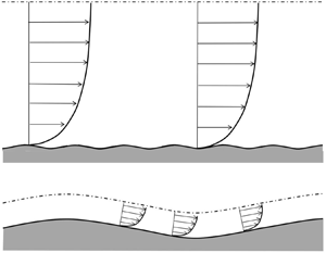
As the in-plane roughness wavelength becomes large relative to the layer thickness ( $\lambda /\delta \rightarrow 1$), the surface will appear more and more heterogeneous to the flow. In effect the outer flow no longer sees the roughness purely in terms of a modified homogeneous boundary condition (a modified
  $U_\tau$) as is the underlying assumption for Townsend's outer-layer similarity argument, but rather will encounter the roughness as a spatially varying
  $U_\tau$ or heterogeneity. It has been well-documented in the literature (for example Hinze Reference Hinze1967; Barros & Christensen Reference Barros and Christensen2014; Willingham et al. Reference Willingham, Anderson, Christensen and Barros2014; Anderson et al. Reference Anderson, Barros, Christensen and Awasthi2015) that spanwise roughness heterogeneity can lead to the formation of Prandtl's secondary flows of the second kind (Bradshaw Reference Bradshaw1987), with recent evidence suggesting that the strength of these secondary flows is a strong function of the outer-scaled heterogeneity wavelength
  $\lambda _h / \delta$, reaching a maximum strength for
  $\lambda _h / \delta \approx 2$ (Anderson et al. Reference Anderson, Yang, Shrestha and Awasthi2018; Chung et al. Reference Chung, Monty and Hutchins2018; Medjnoun et al. Reference Medjnoun, Vanderwel and Ganapathisubramani2018; Yang & Anderson Reference Yang and Anderson2018; Wangsawijaya et al. Reference Wangsawijaya, Baidya, Chung, Marusic and Hutchins2020). These same studies also show that the size of the secondary flows is dependent on the spanwise length scale
  $\lambda _h$, with finer spanwise spacing confining the secondary flows and subsequent spanwise variations to the region closer to the wall, while when
  $\lambda _h / \delta \rightarrow 2$ the secondary flows become space filling and the spanwise variations in the mean extend throughout the majority of the boundary layer. A recent numerical study by Chan et al. (Reference Chan, MacDonald, Chung, Hutchins and Ooi2018) of homogeneous roughness has shown that the wall-normal extent of the dispersive stresses (the extent of the spanwise three-dimensionality induced by the secondary flows) is a direct function of the spanwise wavelength (for an egg-carton type three-dimensional roughness). This study shows that the thickness of the roughness sublayer (defined as the region where the flow from individual roughness elements extends) is a direct function of spanwise in-plane roughness wavelength. When this wavelength approaches
  $\delta$, the roughness sublayer can start to fill the layer. As evidence of this behaviour, figures 6(a) and 6(b) plots the fractional variation in the local mean
  $U (y,z)$ about the spanwise average mean
  $\langle U \rangle (z)$ for both the
  $2.5\times$ and
  $15\times$ surfaces, respectively (this is the dispersive component
  $\tilde {u}$ as a fraction of
  $\langle U \rangle (z)$). It is clear that the fractional variation across the span is much more pronounced for the
  $15\times$ surface, with stronger fluctuations extending farther from the wall. From their analysis of egg-carton type regular rough surfaces, Chan et al. (Reference Chan, MacDonald, Chung, Hutchins and Ooi2018) suggest that the dispersive stresses will extend to approximately
  $z = 0.5\lambda _{y}$, which is shown by the dot-dashed line on figure 6. It is clear that this limit approximately describes the wall-normal extent of the strong spanwise variations for the
  $15\times$ case. For reference the mean wavelength
  $\lambda$ of the two scaled surfaces is also represented on the plots, and it can be seen that the average spanwise length scale of the mean velocity variations in figure 6(b) is close to this wavelength. The boundary layer thickness
  $\delta$ is shown by the dashed line, which shows little difference in spanwise variation for either case, in keeping with the observation that the roughness sublayer only extends to approximately half of the boundary layer thickness for the
  $15\times$ case, and thus has not strongly influenced the overall layer thickness. Morgan & McKeon (Reference Morgan and McKeon2018) studied wall-bounded turbulence over a singly periodic sinusoidal roughness with in-plane wavelengths of the order of the boundary layer thickness, noting that the roughness sublayer extended far into the wake region (
 $z/\delta \approx 0.6$).

Figure 6. The spanwise variation in the coherent or dispersive streamwise velocity component  $\tilde {u}$ as defined in (2.2) for
  $x = 4$ m and
  $U_\infty = 15\ \textrm{m\ s}^{-1}$. Shaded contours show the variation in the local coherent component normalised by the global mean
  $\tilde {u}/\langle U\rangle \equiv (U - \langle U\rangle )/\langle {U}\rangle$ for the (a)
  $2.5\times$ and (b)
  $15\times$ surfaces. The dot-dashed line shows the approximate limit of the dispersive stresses
  $z = 0.5\lambda _y$ as given by Chan et al. (Reference Chan, MacDonald, Chung, Hutchins and Ooi2018). Dashed lines show spanwise variation in the boundary layer thickness
  $\delta$ and the in-plane roughness wavelength
  $\lambda$ is represented by the included measurement scale.
3.2.2. The onset of the ‘wavy’ regime
Figures 7(a) and 7(b) show a schematic of boundary layers developing over rough surfaces with the same effective slope  $ES_x$ (or equal solidity) but with very different
  $\lambda /\delta$. Note that, for clarity, the sketched effective slope in the schematic (
 $ES\approx 0.2$) is larger than the one tested in this study (
 $ES \approx 0.08$). Figure 7(a) shows a case where
  $\lambda \ll \delta$, for which case the local modifications to the flow due to the surface undulations might be expected to be restricted to the near-wall region, with the average boundary layer thickness (as represented by the dot-dashed line) invariant in
  $x$. This is the standard homogeneous
  $k$-type roughness scenario that is represented by the
  $2.5\times$ surface. Figure 7(b) shows a case where
  $\lambda \gg \delta$. In this limiting case, provided that the effective slope of the surface was sufficiently low such that flow separations were minimised, we might expect a scenario as shown, where the entire boundary layer locally conforms to the surface. In this case the surface undulations no longer appear to the near-wall flow as roughness (there is no roughness generated turbulence close to the surface). In such scenarios we might expect non-
 $k$-type behaviour, with the drag being purely driven (in the limit) by the changes in surface area and by the resultant secondary flows.

Figure 7. Two scenarios with same effective slope  $ES$, but with (a)
  $\lambda _x/\delta < 1$, (b)
  $\lambda _x / \delta \gg 1$, (c) the curve for critical
  $ES$ (
 $\lambda \approx \delta$) as a function of
  $Re_\tau$, for a sinusoidal roughness with
  $k_p^+O(100)$. Symbols show conditions for the
  $15\times$ surface from the current study at both
  $x$ locations (
 $\star$); two-dimensional sinusoidal surfaces of Napoli et al. (Reference Napoli, Armenio and De Marchis2008) (
 $\blacksquare$).
An approach to the fully rough asymptote ( $k$-type behaviour) in the Hama roughness function plots of figures 5 and 8, is typically associated with the dominance of pressure drag over viscous drag. Hence, the different roughness function curves for the two scaled surfaces may suggest that the
  $2.5\times$ surface is more prone to separation and pressure drag. Conversely, the distinct Reynolds number dependence in
  $C_f$ indicated by the roughness function trend for the
  $15\times$ surface suggests that viscous drag should be more dominant in this case. Certainly it is conceivable that for very low
  $ES$ cases the waviness of the surface could become so gradual that viscous effects might still be important regardless of the roughness Reynolds number
  $k^+$. The suggestion from the comparison of the
  $2.5\times$ and
  $15\times$ surfaces is that for surfaces with matched
  $ES$ this dominance of viscous effects might be stronger and the pressure drag effects (and separation) weaker, in cases where
  $\lambda \rightarrow \delta$. It is useful to refer back to the literature at this point. Napoli et al. (Reference Napoli, Armenio and De Marchis2008), Nakato et al. (Reference Nakato, Onogi, Himeno, Tanaka and Suzuki1985) and Schultz & Flack (Reference Schultz and Flack2009) have all suggested that surfaces with low effective slopes can exhibit non-
 $k$-type behaviours, with the former two suggesting that the demarcation could lie somewhere around
  $ES_x \approx 0.15$. Indeed Napoli et al. (Reference Napoli, Armenio and De Marchis2008) found that flow remained attached around roughness elements for
  $ES_x \approx 0.05$, but separated for
  $ES_x \approx 0.15$. The current
  $2.5\times$ and
  $15\times$ scaled surfaces both have equal
  $ES_x \approx 0.08$, lying between these two regimes. One curious aspect of the current result is that the
  $2.5\times$ surface exhibits
  $k$-type behaviour, while the
  $15\times$ surface does not, despite both having the same
  $ES_x$. This perhaps suggests that it is not only
  $ES_x$ that determines the predominance of pressure drag and separation from roughness elements. Along similar lines, Zenklusen et al. (Reference Zenklusen, Kuhn and von Rohr2012) found that whether the flow remained attached or separated from a surface with fixed
  $ES_x = 0.2$ was a function of blockage
  $k_t/H$ or
  $\lambda /\delta$, with attached flow occurring when
  $k_t/H = 1/3$ and
  $\lambda /\delta = 3$. The blockage ratio for the
  $15\times$ surface tested here is much smaller (
 $k_t/\delta \approx 20$) which perhaps suggests that
  $\lambda /\delta$ may be the more important determinant of this behaviour.

Figure 8. Hama roughness function  ${\rm \Delta} U^+$ against the viscous-scaled mean roughness height
  $k_a^+$ for the (open symbols)
  $2.5\times$ and (filled)
  $15\times$ surfaces for both the
  $x = 4$ m (black symbol outline) and
  $x = 2$ m (grey symbol outline). Symbols are as defined in table 1. Dashed line shows fully rough asymptote fitted to the
  $2.5\times$ data,
  ${\rm \Delta} U^+ = \kappa ^{-1}\ln (C k_a^+) + A - B$, where the constant
  $C\approx 2.45$ as determine by least squares fitting.
The scenario shown in figure 7(b) is certainly more extreme than the  $15\times$ surface (where
  $\lambda \approx \delta$), but this conceptual sketch does provide some insight into how surfaces with the same
  $ES_x$, but different
  $\lambda /\delta$, might interact with external boundary layers in very different ways. For the future, in light of the unusual Hama roughness function behaviour for the
  $15\times$ surface, it would be beneficial to compare the separation or pressure drag in the roughness canopy for these surfaces. Laser Doppler anemometry (known as LDA) or index matched particle image velocimetry (PIV) are both candidate measurement techniques that offer access to the roughness canopy and can cope with flow reversals.
If we accept that there is a demarcation between  $k$-type and non-
 $k$-type (or wavy) behaviour that occurs where
  $\lambda$ approaches
  $\delta$, we can perform simple rule-of-thumb calculations to uncover when such scenarios are likely to occur. If we assume a three-dimensional sinusoidal surface (of the type studied by Chan et al. (Reference Chan, MacDonald, Chung, Hutchins and Ooi2015)) we can express the effective slope in the
  $x$ direction as
 \begin{equation} ES_x = \frac{8 k_p^+}{{\rm \pi} \lambda_x^+}, \end{equation}
where  $k_p^+$ is the half-amplitude of the sinusoidal roughness and
  $\lambda _x$ is the streamwise in-plane roughness wavelength. If we assume that
  $\lambda _x/\delta = 1$ at the approximate demarcation between
  $k$-type and non-
 $k$-type behaviour, we can write that
  $\lambda _x^+ = \delta ^+ = Re_\tau$. For most experiments aiming at fully rough conditions,
  $k_p^+$ would be order 100. Hence the critical effective slope
  $ES_{x_{crit}}$ (when
  $\lambda _x = \delta$) can be expressed as
 \begin{equation} ES_{x_{crit}} = \frac{8 k_p^+}{{\rm \pi} Re_\tau} \approx \frac{255}{Re_\tau}. \end{equation}
Though this is for a single mode three-dimensional sinusoidal surface, and though the actual value of  $k_p^+$ is unknown, (3.3) can show some important properties (if we accept that
  $\lambda \to \delta$ demarcates roughness regimes). Equation (3.3) is plotted in figure 7(c). Since the demarcation
  $\lambda \to \delta$ is indistinct, due to the need to assume a value for
  $k_p^+$, we represent the proposed transition between roughness regimes with a hatched region representing
  $50 < k_p^+ < 150$. The grey shaded region in figure 7(c) shows the region of the parameter space where
  $\lambda < \delta$, while the white shaded region shows
  $\lambda > \delta$. Figure 7(c) demonstrates that for high Reynolds numbers, we would in general require abnormally low
  $ES$ to see
  $\lambda _x/\delta$ approach unity (under the present assumptions for the sinusoidal surface,
  $ES_{x_{crit}} \approx 0.025$ at
  $Re_\tau = 10\,000$). However, at lower
  $Re_\tau$, more realistic
  $ES_x$ will meet this waviness criteria as fully rough conditions are approached (
 $ES_{x_{crit}} = 0.255$ at
  $Re_\tau = 1000$). Certainly, for the present
  $15\times$ data, it is the combination of low
  $ES_x$, relatively large roughness height
  $k_p$ and low-to-moderate
  $Re$ that have caused
  $\lambda /\delta$ to approach unity. Conditions from the present study for the
  $15\times$ surface at
  $x = 2$ and
  $x = 4$ m are included in figure 7(c) as the filled star symbols. It is clear that these data encroach on the region of the
  $Re_\tau$ and
  $ES$ parameter space where we expect
  $\lambda \approx \delta$ (the
  $15\times$ surface has nominal
  $\lambda /\delta = 1.4$ at
  $x = 2$ m and
  $\lambda /\delta = 0.8$ at
  $x = 4$ m). The filled square symbol in figure 7(c) is case
  $c_8$ from Napoli et al. (Reference Napoli, Armenio and De Marchis2008), which is a single mode two-dimensional sinusoid with
  $\lambda /\delta = 2{\rm \pi}$. Napoli et al. (Reference Napoli, Armenio and De Marchis2008) reported a lower
  ${\rm \Delta} U^+$ for this case than a surface with the same
  $ES$ but much lower
  $k^+$ (case
  $c_1$). It should be reiterated that the
  $\lambda \approx \delta$ curves plotted on figure 7(c) assume a single mode egg-carton type sinusoidal surface with
  $k^+$
$k^+$  $O(100)$. The surfaces and conditions of Napoli et al. (Reference Napoli, Armenio and De Marchis2008) do not conform to these idealised assumptions. Nonetheless, the parameter-space map of figure 7(c) may be a useful tool for collating rough surfaces that exhibit non-classical behaviour. An alternative form of (3.3) is that
  $ES_{x_{crit}} = (8/{\rm \pi} )(k_p/\delta )$, which indicates that the critical
  $ES_x$ is only likely to be abnormally low in situations where
  $k_p/\delta$ is very small (a scenario that usually necessitates high
  $Re$ to achieve fully rough conditions). For more typical values of
  $k_p/\delta$ (say
  $0.025\text {--}0.05$, typical of many laboratory scale facilities),
  $\lambda /\delta$ may approach unity at much higher values of
  $ES_x$.
3.3. A possible $d$-type behaviour

Figure 8 shows the Hama roughness function for both the  $x = 2$ and
  $x = 4$ m measurements. Considering first the
  $2.5\times$ results, it is clear that this smaller scaled surface behaves in a
  $k$-type manner. The values of
  ${\rm \Delta} U^+$ and
  $k_a^+$ are slightly higher at matched
  $U_\infty$ for the
  $x = 2$ m data, as compared with the
  $x = 4$ m cases, however, this is simply due to the variation of
  $C_f$ with
  $x$ for a developing turbulent boundary layer (see for example Monty et al. Reference Monty, Dogan, Hanson, Scardino, Ganapathisubramani and Hutchins2016). The important point for the
  $2.5\times$ case is that when plotted in this manner, the variation of
  ${\rm \Delta} U^+$ with
  $k_a^+$ for both streamwise locations conforms to the same
  $k$-type fully rough asymptote. The
  $15\times$ data shows a more surprising tendency. In some respects the
  $x = 2$ m data confirms the previously observed behaviour for the
  $15\times$ surface at
  $x = 4$ m. The growth of the roughness function with
  $k_a^+$ no longer seems to be tending to the fully rough asymptote and also, despite the sixfold increase in
  $k_a^+$, the Hama roughness function for the
  $15\times$ surface is no larger than for the
  $2.5\times$ surface. The added complication in the behaviour is that in general the
  ${\rm \Delta} U^+$ for the
  $x = 2$ m data are higher than the
  $x = 4$ m data, despite the fact that viscous-scaled roughness height
  $k_a^+$ is approximately comparable between cases. This again is strongly indicative of non-
 $k$-type behaviour. For the
  $15\times$ surface,
  $\lambda /\delta \approx 0.8$ for the
  $x = 4$ m measurements, rising to
  $\lambda /\delta \approx 1.4$ for the
  $x = 2$ m cases. The difference in
  ${\rm \Delta} U^+$ at these different streamwise locations (with very different boundary layer thicknesses) suggests that as
  $\lambda /\delta$ approaches unity, it is the ratio
  $\lambda /\delta$ and not the viscous scaled roughness height
  $k^+$ that determines the drag penalty
  ${\rm \Delta} U^+$. In this sense the comparison shown in figure 8 is suggestive of the
  $d$-type regime suggested by Perry and coworkers (Perry et al. Reference Perry, Schofield and Joubert1969).
4. Conclusions
From these results, it is clear that although we keep  $ES_x$ constant, geometrically scaling a roughness to obtain larger
  $k_a$ does not necessarily lead to a surface that is dynamically ‘rougher’. The subtlety here is that when we scale surfaces geometrically in all dimensions, in addition to making
  $k$ larger, the in-plane wavelength of the roughness
  $\lambda$ relative to the turbulent boundary layer thickness
  $\delta$ is also increased. It would appear that when this wavelength becomes an appreciable proportion of the boundary layer thickness, the surface ceases to behave in a ‘
 $k$-type’ manner. As
  $\lambda$ approaches
  $\delta$, the roughness function (and hence drag penalty) ceases to scale with
  $k$, showing signs instead of scaling with
  $\lambda /\delta$. We show that in this condition, large-scale secondary flows (or regions of dispersive stress) form, which in the
  $15\times$ case permeate the lower half of the boundary layer possibly affecting the dynamics in the logarithmic region. Ultimately, one might imagine that as
  $\lambda$ becomes much greater than the boundary layer thickness, the flow may experience the roughness in a very different manner as the entire boundary layer starts to ‘ride over’ the undulations (as represented schematically in figure 7a). In the future, a more systematic investigation that involves several additional
  $\lambda /\delta$ will be required to provide a better understanding of this behaviour. In addition, based on observations from the
  ${\rm \Delta} U^+$ curves, which suggest that the
  $15\times$ case is less dominated by pressure drag, it would be useful to document any changes in flow separation about the roughness elements that might occur as
  $\lambda /\delta \rightarrow 1$.
Ultimately, the critical behaviour demonstrated here as  $\lambda /\delta$ approaches unity suggests caution should be exercised when attempting to replicate the viscous-scaled roughness condition from a large (high
  $Re$) engineering application in a much lower
  $Re$ laboratory facility or numerical simulation (particularly where the facility has a very different unit Reynolds number
  $U_\infty /\nu$). As an example, the
  $15\times$ scaled surface that led to the anomalous behaviour reported here resulted from an attempt to scale a scanned ship's hull roughness (resulting from spray painting application) to attain fully rough behaviour in a small-scale wind tunnel. Typically, we scale surfaces because we wish to match viscous-scaled roughness heights obtained in the laboratory to those encountered in application. However, because the
  $Re_\tau$ in the laboratory (or simulation) is often so much lower than the application Reynolds number, there is a danger for low effective slope surfaces that
  $\lambda$ will approach the outer length scale
  $\delta$. Results presented in this study suggest that drag predictions will suffer when this condition is artificially imposed through scaling. There are, however, likely to be other cases in engineering and meteorological applications where
  $\lambda$ is equivalent to the outer length scale. The stable boundary layer over long wavelength ocean waves provides one possible example, as do thin boundary layers developing over low effective slope engineering surfaces (resulting, say, from spray coating or manufacturing processes), such as narrow internal cooling channels in heat exchangers.
Acknowledgements
The authors would like to thank the Australian Research Council and the Newton Fund for the support of this work. B.G. is grateful to EPSRC for their support through grant EP/P009638/1. The authors thank Mr M. Yusuf from PT Dharma Lautan Utama for providing access to the Dharma Kencana IX ferry, Dr M. Tullberg of Hempel A/S for his assistance in obtaining the hull roughness imprint and Dr F.A. Prasetyo from PT Biro Klasifikasi Indonesia for ensuring the safety of our research team. All data supporting this study are openly available from the University of Southampton repository at https://doi.org/10.5258/SOTON/D1559.
Declaration of interests
The authors report no conflict of interest.


