1 Introduction
The inverse cascade, acting on balanced ocean macroturbulence, transfers energy towards large spatial scales. However, a statistically steady ocean circulation requires energy dissipation at the same rate as it is supplied by the wind. Thus equilibration of the ocean macroturbulence requires ageostrophic processes, acting in opposition to the inverse cascade, to produce a transfer of energy towards the centimetre scales at which molecular viscosity is effective. Mechanisms that might result in this down-scale transfer include, but are not limited to, surface and benthic boundary-layer turbulence, lee-wave generation by mesoscale eddies negotiating bottom topography and the spontaneous generation of internal waves by upper-ocean frontal instabilities; see Nagai et al. (Reference Nagai, Tandon, Kunze and Mahadevan2015) for a recent review.
Table 1. Summary of model-based studies of energy extraction from balanced flow by near-inertial waves.

We focus on a mechanism first identified by Gertz & Straub (Reference Gertz and Straub2009): externally forced near-inertial waves might provide an energy sink for large-scale balanced flow. Since Gertz & Straub (Reference Gertz and Straub2009), several other studies, summarized in table 1, have argued for significant energy transfer from balanced flows to near-inertial waves. A common aspect of the studies in table 1 is that the near-inertial waves are first introduced by external forcing (e.g. wind) at the inertial frequency and then grow by extracting energy from the balanced flow.
(An exception in table 1 is the study of Shakespeare & Hogg (Reference Shakespeare and Hogg2017), in which near-inertial waves are generated spontaneously – without external forcing – at density fronts near the surface. These waves then radiate vertically downwards into the interior and amplify by extracting energy from deep balanced flow. We have included Shakespeare & Hogg (Reference Shakespeare and Hogg2017) in table 1 because, as far as deep interior amplification is concerned, the details of the shallow generation process are probably immaterial.)
The studies in table 1 have shown that externally generated near-inertial waves can extract energy from a pre-existing balanced flow. Those studies, however, have diverse methodology and diagnostic framework, so there is not a consensus that the observed amplification of near-inertial waves results from a single mechanism. In other words, it is possible that near-inertial wave amplification occurs through a variety of mechanisms and each instance must be analysed and understood on its own peculiar terms. But in a certain limit, described in § 2.2, there is a single underlying mechanism – stimulated generation – that is responsible for energy transfer between waves and balanced flow (Xie & Vanneste Reference Xie and Vanneste2015, XV hereafter). While it is unclear whether this limit applies to the studies in table 1, XV provide a robust yet simple theoretical framework for studying energy transfers between balanced flows and near-inertial waves.
Using a variational formulation of the generalized Lagrangian mean, XV derived a phase-averaged model of the coupling between weakly nonlinear near-inertial waves and quasi-geostrophic (QG) flow. Wagner & Young (Reference Wagner and Young2016) derived a similar coupled model via Eulerian multiple-time expansion; these authors include the second harmonic of the primary near-inertial wave and simplify the wave dynamics by assuming moderate QG vertical shears. In both coupled models the near-inertial waves (NIW) are governed by the equation of Young & Ben Jelloul (Reference Young and Ben Jelloul1997) (YBJ hereafter) and the balanced flow satisfies QG dynamics – the waves contribute phase-averaged quadratic terms of the same order as the QG potential vorticity (PV). Salmon (Reference Salmon2016) provides a useful perspective on this ‘NIW-QG’ model; without assuming that the waves are near-inertial, and within a single variational framework, Salmon unifies XV’s model with the wave-mean flow models of Bühler & McIntyre (Reference Bühler and McIntyre1998) and Wagner & Young (Reference Wagner and Young2015). Salmon also emphasizes a revealing analogy between vortex–wave interactions and classical electrodynamics.
To distinguish energy extraction by existing waves from spontaneous generation, and to complete an electrodynamic analogy, XV refer to the transfer of energy from balanced flow to externally forced near-inertial waves as stimulated generation. The more widely studied process of spontaneous generation is the emission of internal waves arising from the slow evolution of balanced flow in the absence of external forcing at wave frequencies (Vanneste Reference Vanneste2013). Spontaneous generation is inefficient at small and moderate Rossby numbers and its global impact on ocean energetics is probably small (Danioux et al. Reference Danioux, Vanneste, Klein and Sasaki2012; Nagai et al. Reference Nagai, Tandon, Kunze and Mahadevan2015). Also, spontaneous generation is localized at sharp submesoscale fronts with order-one Rossby number (e.g. Shakespeare & Hogg Reference Shakespeare and Hogg2017) while the stimulated variety operates even at the small Rossby numbers characteristic of most interior oceanic conditions, provided only that internal waves are introduced by external forcing. Throughout the ocean, internal waves are reliably forced by wind and tides and thus stimulated generation is a leading contender as a mesoscale energy sink.
Although XV and Wagner & Young (Reference Wagner and Young2016) use significantly different approaches, their results are consistent with one another. This consistency indicates that the NIW-QG model provides the unique small-amplitude evolution equations describing the interaction between near-inertial waves and geostrophic flow. In the small-amplitude limit the flow can be unambiguously separated into weakly nonlinear internal waves and quasi-geostrophic eddies, with perturbative coupling between waves and eddies (Salmon Reference Salmon2016). To the extent that the studies in table 1 are also in this weak-interaction limit, their results should – in principle – be described by the NIW-QG model. ‘In principle’ because the distinction between the Lagrangian-mean and Eulerian-mean velocities complicates the diagnosis of energy transfers between eddies and waves (see § 6 for further discussion) and because the Rossby number is large in some studies (e.g. Barkan et al. Reference Barkan, Winters and McWilliams2016). Frontal sharpening and low Richardson number processes, which are described in Thomas (Reference Thomas2012), are outside the scope of the NIW-QG model.
XV emphasize that a central feature of the NIW-QG model is that there are two integral energy conservation laws for: (i) near-inertial kinetic energy and (ii) the sum of near-inertial potential energy and total balanced energy. The inevitable reduction of near-inertial length scales by advection and refraction is accompanied by an increase in wave potential energy and, because of conservation law (ii), a reduction in the energy of the balanced flow. These features, and the necessity of an externally forced wave, are the defining characteristics of stimulated generation.
Here we investigate perhaps the simplest example of stimulated generation obtained from the NIW-QG model by assuming barotropic QG flow and vertically planar near-inertial waves. Because the balanced flow is barotropic, while the near-inertial wave is three-dimensional, this ‘vertical-plane-wave model’ resembles the original scenario of Gertz & Straub (Reference Gertz and Straub2009). We show that the convergence of wave kinetic energy into anti-cyclones and geostrophic straining of the waves reduces the wave length scale, amplifies gradients of wave amplitude and converts balanced kinetic energy into near-inertial potential energy.
2 The vertical-plane-wave model
The vertical-plane-wave model is obtained by assuming barotropic balanced flow, with streamfunction
 $\unicode[STIX]{x1D713}(x,y,t)$
, a uniform background buoyancy frequency
$\unicode[STIX]{x1D713}(x,y,t)$
, a uniform background buoyancy frequency
 $N_{0}$
and a single vertically propagating wave with vertical structure
$N_{0}$
and a single vertically propagating wave with vertical structure
 $\text{e}^{\text{i}mz}$
and back-rotated wave velocity
$\text{e}^{\text{i}mz}$
and back-rotated wave velocity
 $\unicode[STIX]{x1D719}(x,y,t)$
. With these idealizations, appendix A derives the vertical-plane-wave model starting from the phase-averaged equations of Wagner & Young (Reference Wagner and Young2016); XV obtain the same model from their version of the phase-averaged equations. In either case, the leading-order wave plus the leading-order balanced velocity
$\unicode[STIX]{x1D719}(x,y,t)$
. With these idealizations, appendix A derives the vertical-plane-wave model starting from the phase-averaged equations of Wagner & Young (Reference Wagner and Young2016); XV obtain the same model from their version of the phase-averaged equations. In either case, the leading-order wave plus the leading-order balanced velocity
 $(u,v,w)$
, pressure
$(u,v,w)$
, pressure
 $p$
and buoyancy
$p$
and buoyancy
 $b$
are
$b$
are
 $$\begin{eqnarray}\displaystyle & \displaystyle u+\text{i}v=\text{e}^{\text{i}\unicode[STIX]{x1D71B}}\,\unicode[STIX]{x1D719}-\unicode[STIX]{x1D713}_{y}+\text{i}\unicode[STIX]{x1D713}_{x}, & \displaystyle\end{eqnarray}$$
 $$\begin{eqnarray}\displaystyle & \displaystyle w=\text{i}m^{-1}\text{e}^{\text{i}\unicode[STIX]{x1D71B}}\,\unicode[STIX]{x2202}\unicode[STIX]{x1D719}+\text{c.c.}, & \displaystyle\end{eqnarray}$$
 $$\begin{eqnarray}\displaystyle & \displaystyle p=-\text{i}\unicode[STIX]{x1D702}\text{e}^{\text{i}\unicode[STIX]{x1D71B}}\,\unicode[STIX]{x2202}\unicode[STIX]{x1D719}+\text{c.c.}+f_{0}\unicode[STIX]{x1D713}, & \displaystyle\end{eqnarray}$$
 $$\begin{eqnarray}\displaystyle & \displaystyle b=m\unicode[STIX]{x1D702}\text{e}^{\text{i}\unicode[STIX]{x1D71B}}\,\unicode[STIX]{x2202}\unicode[STIX]{x1D719}+\text{c.c}. & \displaystyle\end{eqnarray}$$
Above,
 $\unicode[STIX]{x1D71B}=mz-f_{0}t$
is the phase of the vertical plane wave,
$\unicode[STIX]{x1D71B}=mz-f_{0}t$
is the phase of the vertical plane wave,
 $\unicode[STIX]{x1D702}=f_{0}\unicode[STIX]{x1D706}^{2}$
is the wave ‘dispersivity’, where
$\unicode[STIX]{x1D702}=f_{0}\unicode[STIX]{x1D706}^{2}$
is the wave ‘dispersivity’, where
 $\unicode[STIX]{x1D706}=N_{0}/f_{0}\,m$
is a horizontal scale, c.c. denotes complex conjugate and
$\unicode[STIX]{x1D706}=N_{0}/f_{0}\,m$
is a horizontal scale, c.c. denotes complex conjugate and
 $$\begin{eqnarray}\displaystyle & \displaystyle \unicode[STIX]{x2202}\,\stackrel{def}{=}\,{\textstyle \frac{1}{2}}(\unicode[STIX]{x2202}_{x}-\text{i}\unicode[STIX]{x2202}_{y}) & \displaystyle\end{eqnarray}$$
is a differential operator. The complex field
 $\unicode[STIX]{x1D719}(x,y,t)$
in (2.1) is the back-rotated velocity of the near-inertial waves; in (2.2)–(2.4) the other wave fields are expressed in terms of
$\unicode[STIX]{x1D719}(x,y,t)$
in (2.1) is the back-rotated velocity of the near-inertial waves; in (2.2)–(2.4) the other wave fields are expressed in terms of
 $\unicode[STIX]{x2202}\unicode[STIX]{x1D719}$
. The compact representation of the wave variables in terms of
$\unicode[STIX]{x2202}\unicode[STIX]{x1D719}$
. The compact representation of the wave variables in terms of
 $\unicode[STIX]{x1D719}$
follows YBJ.
$\unicode[STIX]{x1D719}$
follows YBJ.
The balanced variables are represented by the streamfunction
 $\unicode[STIX]{x1D713}$
. Because the Stokes pressure correction is negligible for near-inertial waves (Wagner & Young Reference Wagner and Young2016), the eddies are balanced in the sense that
$\unicode[STIX]{x1D713}$
. Because the Stokes pressure correction is negligible for near-inertial waves (Wagner & Young Reference Wagner and Young2016), the eddies are balanced in the sense that
 $\unicode[STIX]{x1D713}=\bar{p}/f_{0}$
, where
$\unicode[STIX]{x1D713}=\bar{p}/f_{0}$
, where
 $\bar{p}$
is either the Eulerian-mean or Lagrangian-mean pressure. Moreover, the velocities obtained from
$\bar{p}$
is either the Eulerian-mean or Lagrangian-mean pressure. Moreover, the velocities obtained from
 $\unicode[STIX]{x1D713}$
in (2.1) are Lagrangian-mean velocities, e.g. the velocity
$\unicode[STIX]{x1D713}$
in (2.1) are Lagrangian-mean velocities, e.g. the velocity
 $(-\unicode[STIX]{x1D713}_{y},\unicode[STIX]{x1D713}_{x})$
advects the material invariant potential vorticity in (2.7) below. We have lightened the notation by using
$(-\unicode[STIX]{x1D713}_{y},\unicode[STIX]{x1D713}_{x})$
advects the material invariant potential vorticity in (2.7) below. We have lightened the notation by using
 $\unicode[STIX]{x1D713}$
, rather than
$\unicode[STIX]{x1D713}$
, rather than
 $\unicode[STIX]{x1D713}^{L}$
; the implicit
$\unicode[STIX]{x1D713}^{L}$
; the implicit
 $L$
is particularly important in § 6.
$L$
is particularly important in § 6.
The PV of the balanced flow is expressed in terms of
 $\unicode[STIX]{x1D713}$
and
$\unicode[STIX]{x1D713}$
and
 $\unicode[STIX]{x1D719}$
by
$\unicode[STIX]{x1D719}$
by
 $$\begin{eqnarray}\displaystyle & \displaystyle q=\underbrace{\unicode[STIX]{x0394}\unicode[STIX]{x1D713}}_{\stackrel{def}{=}\unicode[STIX]{x1D701}}+\underbrace{{\displaystyle \frac{1}{f_{0}}}\left[{\displaystyle \frac{1}{4}}\unicode[STIX]{x0394}|\unicode[STIX]{x1D719}|^{2}+{\displaystyle \frac{\text{i}}{2}}J(\unicode[STIX]{x1D719}^{\star },\unicode[STIX]{x1D719})\right]}_{\stackrel{def}{=}q^{w}}, & \displaystyle\end{eqnarray}$$
where
 $\unicode[STIX]{x0394}\,\stackrel{def}{=}\,\unicode[STIX]{x2202}_{x}^{2}+\unicode[STIX]{x2202}_{y}^{2}$
is the horizontal Laplacian and
$\unicode[STIX]{x0394}\,\stackrel{def}{=}\,\unicode[STIX]{x2202}_{x}^{2}+\unicode[STIX]{x2202}_{y}^{2}$
is the horizontal Laplacian and
 $J(f,g)\,\stackrel{def}{=}\,f_{x}g_{y}-f_{y}g_{x}$
is the Jacobian, and the superscript star
$J(f,g)\,\stackrel{def}{=}\,f_{x}g_{y}-f_{y}g_{x}$
is the Jacobian, and the superscript star
 $^{\star }$
denotes complex conjugation. Equation (2.6) is the ‘inversion relation’:
$^{\star }$
denotes complex conjugation. Equation (2.6) is the ‘inversion relation’:
 $q$
and
$q$
and
 $\unicode[STIX]{x1D719}$
determine the Lagrangian-mean flow via
$\unicode[STIX]{x1D719}$
determine the Lagrangian-mean flow via
 $\unicode[STIX]{x1D713}=\unicode[STIX]{x0394}^{-1}(q-q^{w})$
where
$\unicode[STIX]{x1D713}=\unicode[STIX]{x0394}^{-1}(q-q^{w})$
where
 $q^{w}$
defined in (2.6) is the ‘wave potential vorticity’. Once
$q^{w}$
defined in (2.6) is the ‘wave potential vorticity’. Once
 $\unicode[STIX]{x1D713}$
is obtained by inversion, the field equations (2.7) and (2.8) below can be time-stepped.
$\unicode[STIX]{x1D713}$
is obtained by inversion, the field equations (2.7) and (2.8) below can be time-stepped.
Using the generalized Lagrangian-mean formulation, Bühler & McIntyre (Reference Bühler and McIntyre1998) showed that the assumption of weak interaction between internal waves and balanced flow results in wave-averaged term
 $q^{w}$
contributing to the materially conserved PV; see also Grimshaw (Reference Grimshaw1975). In (2.6) the wave-averaged feedback on the balanced flow is expressed concisely in terms of the back-rotated velocity
$q^{w}$
contributing to the materially conserved PV; see also Grimshaw (Reference Grimshaw1975). In (2.6) the wave-averaged feedback on the balanced flow is expressed concisely in terms of the back-rotated velocity
 $\unicode[STIX]{x1D719}$
via the quadratic terms in
$\unicode[STIX]{x1D719}$
via the quadratic terms in
 $q^{w}$
.
$q^{w}$
.
2.1 The evolution equations
The balanced flow evolves according to PV advection
 $$\begin{eqnarray}\displaystyle & \displaystyle q_{t}+J(\unicode[STIX]{x1D713},q)=D_{q}; & \displaystyle\end{eqnarray}$$
the back-rotated velocity satisfies the wave equation
 $$\begin{eqnarray}\displaystyle & \displaystyle \unicode[STIX]{x1D719}_{t}+J(\unicode[STIX]{x1D713},\unicode[STIX]{x1D719})+\unicode[STIX]{x1D719}{\displaystyle \frac{\text{i}}{2}}\unicode[STIX]{x1D701}-{\displaystyle \frac{\text{i}}{2}}\unicode[STIX]{x1D702}\unicode[STIX]{x0394}\unicode[STIX]{x1D719}=D_{\unicode[STIX]{x1D719}}. & \displaystyle\end{eqnarray}$$
 $D_{q}$
and
$D_{q}$
and
 $D_{\unicode[STIX]{x1D719}}$
in (2.7) and (2.8) are dissipative terms described below.
$D_{\unicode[STIX]{x1D719}}$
in (2.7) and (2.8) are dissipative terms described below.
The wave equation (2.8) is the YBJ model in the case where the near-inertial wave has
 $\text{e}^{\text{i}mz}$
structure. The back-rotated wave velocity,
$\text{e}^{\text{i}mz}$
structure. The back-rotated wave velocity,
 $\unicode[STIX]{x1D719}$
, evolves through dispersion – the last term on the left of (2.8) – and nonlinear advection and refraction by the second and third terms in (2.8). Without advection, (2.8) is analogous to Schrödinger’s equation (e.g. Landau & Lifshitz Reference Landau and Lifshitz2013, p. 51). The relative vorticity,
$\unicode[STIX]{x1D719}$
, evolves through dispersion – the last term on the left of (2.8) – and nonlinear advection and refraction by the second and third terms in (2.8). Without advection, (2.8) is analogous to Schrödinger’s equation (e.g. Landau & Lifshitz Reference Landau and Lifshitz2013, p. 51). The relative vorticity,
 $\unicode[STIX]{x1D701}=\unicode[STIX]{x0394}\unicode[STIX]{x1D713}$
, is the potential, with negative
$\unicode[STIX]{x1D701}=\unicode[STIX]{x0394}\unicode[STIX]{x1D713}$
, is the potential, with negative
 $\unicode[STIX]{x1D701}$
a well, and the ‘dispersivity’,
$\unicode[STIX]{x1D701}$
a well, and the ‘dispersivity’,
 $f_{0}\unicode[STIX]{x1D706}^{2}$
, is Planck’s constant (Balmforth, Llewellyn Smith & Young Reference Balmforth, Llewellyn Smith and Young1998; Balmforth & Young Reference Balmforth and Young1999; Danioux, Vanneste & Bühler Reference Danioux, Vanneste and Bühler2015). The quantum analogy may be useful for some readers, but it is not necessary for the understanding of the results below.
$f_{0}\unicode[STIX]{x1D706}^{2}$
, is Planck’s constant (Balmforth, Llewellyn Smith & Young Reference Balmforth, Llewellyn Smith and Young1998; Balmforth & Young Reference Balmforth and Young1999; Danioux, Vanneste & Bühler Reference Danioux, Vanneste and Bühler2015). The quantum analogy may be useful for some readers, but it is not necessary for the understanding of the results below.
The terms on the right of (2.7) and (2.8),
 $D_{q}$
and
$D_{q}$
and
 $D_{\unicode[STIX]{x1D719}}$
, represent small-scale dissipation. Small-scale dissipation is necessary to absorb the forward transfers of potential enstrophy and wave kinetic and potential energies in the numerical solutions reported below. We find that biharmonic diffusion and viscosity,
$D_{\unicode[STIX]{x1D719}}$
, represent small-scale dissipation. Small-scale dissipation is necessary to absorb the forward transfers of potential enstrophy and wave kinetic and potential energies in the numerical solutions reported below. We find that biharmonic diffusion and viscosity,
 $$\begin{eqnarray}\displaystyle & \displaystyle D_{q}=-\unicode[STIX]{x1D705}_{e}\unicode[STIX]{x0394}^{2}q\quad \text{and}\quad D_{\unicode[STIX]{x1D719}}=-\unicode[STIX]{x1D708}_{\unicode[STIX]{x1D719}}\unicode[STIX]{x0394}^{2}\unicode[STIX]{x1D719}, & \displaystyle\end{eqnarray}$$
are sufficient to extend the spectral resolution compared to Laplacian dissipation. In practice, we choose
 $\unicode[STIX]{x1D705}_{e}$
and
$\unicode[STIX]{x1D705}_{e}$
and
 $\unicode[STIX]{x1D708}_{\unicode[STIX]{x1D719}}$
so that the highest 35 % of the modes lie in the dissipation range and aliased wavenumbers are strongly damped.
$\unicode[STIX]{x1D708}_{\unicode[STIX]{x1D719}}$
so that the highest 35 % of the modes lie in the dissipation range and aliased wavenumbers are strongly damped.
2.2 The small-amplitude limit and the validity of the NIW-QG approximation
The development of the NIW-QG model is ordered first by assuming that the waves are weak in the sense that
 $$\begin{eqnarray}\displaystyle & \displaystyle \unicode[STIX]{x1D716}\,\stackrel{def}{=}\,{\displaystyle \frac{U_{w}}{f_{0}L}}\ll 1. & \displaystyle\end{eqnarray}$$
Above,
 $L$
is a characteristic scale of both waves and balanced flow and
$L$
is a characteristic scale of both waves and balanced flow and
 $U_{w}$
is a characteristic near-inertial wave velocity. The other small parameter in the expansion is the Rossby number of the balanced flow,
$U_{w}$
is a characteristic near-inertial wave velocity. The other small parameter in the expansion is the Rossby number of the balanced flow,
 $$\begin{eqnarray}\displaystyle & \displaystyle Ro\,\stackrel{def}{=}\,{\displaystyle \frac{U_{e}}{f_{0}L}}\ll 1, & \displaystyle\end{eqnarray}$$
where
 $U_{e}$
is the eddy velocity. The inequalities in (2.10) and (2.11) must be satisfied in order to obtain the NIW-QG system. But XV and Wagner & Young (Reference Wagner and Young2016) make a third assumption:
$U_{e}$
is the eddy velocity. The inequalities in (2.10) and (2.11) must be satisfied in order to obtain the NIW-QG system. But XV and Wagner & Young (Reference Wagner and Young2016) make a third assumption:
 $Ro=\unicode[STIX]{x1D716}^{2}$
, or equivalently that
$Ro=\unicode[STIX]{x1D716}^{2}$
, or equivalently that
 $U_{e}=\unicode[STIX]{x1D716}U_{w}$
. The resulting distinguished limit,
$U_{e}=\unicode[STIX]{x1D716}U_{w}$
. The resulting distinguished limit,
 $$\begin{eqnarray}\displaystyle & \displaystyle \unicode[STIX]{x1D716}\rightarrow 0,\quad \text{with}~Ro=\unicode[STIX]{x1D716}^{2}, & \displaystyle\end{eqnarray}$$
promotes the importance of wave-averaged effects so that
 $q^{w}$
appears at an early, and accessible, order in the expansion. Thus (2.12) is for convenience rather than necessity.
$q^{w}$
appears at an early, and accessible, order in the expansion. Thus (2.12) is for convenience rather than necessity.
The asymptotic ordering in (2.12) does not imply that the NIW-QG system fails for weaker waves, i.e. if
 $U_{w}$
is comparable to, or even smaller than,
$U_{w}$
is comparable to, or even smaller than,
 $U_{e}$
. Making
$U_{e}$
. Making
 $U_{w}$
weaker than
$U_{w}$
weaker than
 $U_{e}$
delays wave-averaged effects to longer times – it does not, per se, invalidate the expansion. The main problem with the weak-wave limit is that other physics, not considered in the NIW-QG system, will contend with wave-averaged effects on ultra-long time scales. For example, even without waves, order-
$U_{e}$
delays wave-averaged effects to longer times – it does not, per se, invalidate the expansion. The main problem with the weak-wave limit is that other physics, not considered in the NIW-QG system, will contend with wave-averaged effects on ultra-long time scales. For example, even without waves, order-
 $Ro^{2}$
ageostrophic effects modify the evolution of balanced flow and produce departures from QG (e.g. see Muraki, Snyder & Rotunno Reference Muraki, Snyder and Rotunno1999).
$Ro^{2}$
ageostrophic effects modify the evolution of balanced flow and produce departures from QG (e.g. see Muraki, Snyder & Rotunno Reference Muraki, Snyder and Rotunno1999).
To summarize: the main conditions for the validity of the NIW-QG system are (2.10) and (2.11); additionally, validity of the wave equation (2.8) requires that the wave frequency is close of
 $f_{0}$
. The weak-wave limit
$f_{0}$
. The weak-wave limit
 $U_{w}/U_{e}\rightarrow 0$
is valid within the NIW-QG framework: in that limit the system reduces to the barotropic potential vorticity equation and the YBJ equation for a passive wave field.
$U_{w}/U_{e}\rightarrow 0$
is valid within the NIW-QG framework: in that limit the system reduces to the barotropic potential vorticity equation and the YBJ equation for a passive wave field.
The standard QG approximation is used successfully even when
 $Ro\sim 1$
(Hoskins Reference Hoskins1975) and we expect the NIW-QG model to enjoy similar success if
$Ro\sim 1$
(Hoskins Reference Hoskins1975) and we expect the NIW-QG model to enjoy similar success if
 $\ll$
is replaced by
$\ll$
is replaced by
 ${<}$
in (2.11). Flows with
${<}$
in (2.11). Flows with
 $Ro>1$
eddies, such as those reported in Barkan et al. (Reference Barkan, Winters and McWilliams2016), evolve on time scales close to
$Ro>1$
eddies, such as those reported in Barkan et al. (Reference Barkan, Winters and McWilliams2016), evolve on time scales close to
 $f_{0}^{-1}$
, and an Eulerian decomposition into near-inertial waves and eddies is ill-defined unless there is spatial scale separation between eddies and waves. These large Rossby number flows are outside the purview of the NIW-QG model (XV; Wagner & Young Reference Wagner and Young2016).
$f_{0}^{-1}$
, and an Eulerian decomposition into near-inertial waves and eddies is ill-defined unless there is spatial scale separation between eddies and waves. These large Rossby number flows are outside the purview of the NIW-QG model (XV; Wagner & Young Reference Wagner and Young2016).
2.3 An illustrative solution: the Lamb–Chaplygin dipole
As a preamble to our discussion of stimulated generation in freely evolving two-dimensional turbulence, we consider an example in which the initial QG flow is the Lamb–Chaplygin dipole; see figure 1. This dipole is an exact solution of the Euler equations on an infinite two-dimensional plane where the vorticity is confined to a circle of radius
 $R$
(Meleshko & Van Heijst Reference Meleshko and Van Heijst1994). The relative vorticity, steady in a frame moving at uniform zonal velocity
$R$
(Meleshko & Van Heijst Reference Meleshko and Van Heijst1994). The relative vorticity, steady in a frame moving at uniform zonal velocity
 $U_{e}$
, is
$U_{e}$
, is
 $$\begin{eqnarray}\displaystyle & \displaystyle \unicode[STIX]{x1D701}={\displaystyle \frac{2U_{e}\unicode[STIX]{x1D705}}{\text{J}_{0}(\unicode[STIX]{x1D705}R)}}\left\{\begin{array}{@{}ll@{}}\text{J}_{1}(\unicode[STIX]{x1D705}r)\sin \unicode[STIX]{x1D703},\quad & \text{if }r\leqslant R,\\ 0,\quad & \text{if }r\geqslant R.\end{array}\right. & \displaystyle\end{eqnarray}$$
Above
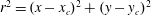 $r^{2}=(x-x_{c})^{2}+(y-y_{c})^{2}$
is the radial distance from the centre
$r^{2}=(x-x_{c})^{2}+(y-y_{c})^{2}$
is the radial distance from the centre
 $(x_{c},y_{c})$
,
$(x_{c},y_{c})$
,
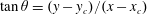 $\tan \unicode[STIX]{x1D703}=(y-y_{c})/(x-x_{c})$
and
$\tan \unicode[STIX]{x1D703}=(y-y_{c})/(x-x_{c})$
and
 $\text{J}_{n}$
is the
$\text{J}_{n}$
is the
 $n$
th-order Bessel function. The matching condition at
$n$
th-order Bessel function. The matching condition at
 $r=R$
is that
$r=R$
is that
 $\text{J}_{1}(\unicode[STIX]{x1D705}R)=0$
and the smallest solution is
$\text{J}_{1}(\unicode[STIX]{x1D705}R)=0$
and the smallest solution is
 $\unicode[STIX]{x1D705}R\approx 3.8317$
. If there is no coupling to the wave
$\unicode[STIX]{x1D705}R\approx 3.8317$
. If there is no coupling to the wave
 $\unicode[STIX]{x1D719}$
, then the dipole (2.13) is a solution of the QG equation (2.7).
$\unicode[STIX]{x1D719}$
, then the dipole (2.13) is a solution of the QG equation (2.7).

Figure 1. Snapshots of the Lamb–Chaplygin dipole solution with parameters presented in table 2. Contours depict potential vorticity,
 $q/(U_{e}k_{e})=[-1.5,-0.5,0.5,1.5]$
, with dashed lines showing negative values. (a–c) The wave action density
$q/(U_{e}k_{e})=[-1.5,-0.5,0.5,1.5]$
, with dashed lines showing negative values. (a–c) The wave action density
 $|\unicode[STIX]{x1D719}|^{2}/2f_{0}$
. (d–f) The wave buoyancy; the buoyancy scale is
$|\unicode[STIX]{x1D719}|^{2}/2f_{0}$
. (d–f) The wave buoyancy; the buoyancy scale is
 $B=k_{e}mU_{w}f_{0}\unicode[STIX]{x1D706}^{2}$
. These plots only show the central
$B=k_{e}mU_{w}f_{0}\unicode[STIX]{x1D706}^{2}$
. These plots only show the central
 $(1/5)^{2}$
of the simulation domain.
$(1/5)^{2}$
of the simulation domain.
Table 2. Description of parameters of Lamb–Chaplygin simulation. The initial conditions are Rossby number
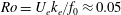 $Ro=U_{e}k_{e}/f_{0}\approx 0.05$
, wave dispersivity
$Ro=U_{e}k_{e}/f_{0}\approx 0.05$
, wave dispersivity
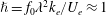 $\hslash =f_{0}\unicode[STIX]{x1D706}^{2}k_{e}/U_{e}\approx 1$
and wave amplitude
$\hslash =f_{0}\unicode[STIX]{x1D706}^{2}k_{e}/U_{e}\approx 1$
and wave amplitude
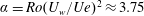 $\unicode[STIX]{x1D6FC}=Ro(U_{w}/Ue)^{2}\approx 3.75$
.
$\unicode[STIX]{x1D6FC}=Ro(U_{w}/Ue)^{2}\approx 3.75$
.

We strongly perturb the dipole in (2.13) by seeding a wave with initial velocity:
 $$\begin{eqnarray}\displaystyle & \displaystyle \unicode[STIX]{x1D719}(x,y,t=0)={\displaystyle \frac{1+\text{i}}{\sqrt{2}}}\,U_{w}. & \displaystyle\end{eqnarray}$$
If there was no dipole, this initial condition produces a spatially uniform near-inertial oscillation with speed
 $U_{w}$
. Further parameters of this solution are summarized in table 2; note
$U_{w}$
. Further parameters of this solution are summarized in table 2; note
 $U_{w}=10U_{e}$
.
$U_{w}=10U_{e}$
.
We integrate the vertical-plane-wave model using a standard collocation Fourier spectral method. We evaluate the quadratic nonlinearities, including in the wave potential vorticity (2.6), in physical space, and transform the product into Fourier space. We time march the spectral equations using an exponential time differencing method with a fourth-order Runge–Kutta scheme – for details, see Cox & Matthews (Reference Cox and Matthews2002) and Kassam & Trefethen (Reference Kassam and Trefethen2005).
With the initial condition in (2.14),
 $q^{w}$
in (2.6) and
$q^{w}$
in (2.6) and
 $\unicode[STIX]{x1D735}\unicode[STIX]{x1D719}$
are both zero at
$\unicode[STIX]{x1D735}\unicode[STIX]{x1D719}$
are both zero at
 $t=0$
. The refractive term in the wave equation (2.8), however, immediately imprints itself onto
$t=0$
. The refractive term in the wave equation (2.8), however, immediately imprints itself onto
 $\unicode[STIX]{x1D719}$
thus creating non-zero
$\unicode[STIX]{x1D719}$
thus creating non-zero
 $\unicode[STIX]{x1D735}\unicode[STIX]{x1D719}$
and non-zero
$\unicode[STIX]{x1D735}\unicode[STIX]{x1D719}$
and non-zero
 $q^{w}$
. Once refraction has created gradients in
$q^{w}$
. Once refraction has created gradients in
 $\unicode[STIX]{x1D719}$
, the advective term in (2.8) can further distort
$\unicode[STIX]{x1D719}$
, the advective term in (2.8) can further distort
 $\unicode[STIX]{x1D719}$
and increase
$\unicode[STIX]{x1D719}$
and increase
 $\unicode[STIX]{x1D735}\unicode[STIX]{x1D719}$
. This scale reduction of
$\unicode[STIX]{x1D735}\unicode[STIX]{x1D719}$
. This scale reduction of
 $\unicode[STIX]{x1D719}$
is most evident in the wave buoyancy shown in figure 1(d–f). Figure 1 also shows the well-known focusing of waves into the negative vortex. But the wave feedback on the mean flow through
$\unicode[STIX]{x1D719}$
is most evident in the wave buoyancy shown in figure 1(d–f). Figure 1 also shows the well-known focusing of waves into the negative vortex. But the wave feedback on the mean flow through
 $q^{w}$
then results in distortion and shearing of the dipole so that the negative vortex loses its integrity; the lopsided dipole then starts to drift. Once the negative vortex is distorted to small scales it no longer acts as an effective potential well: the trapping of wave energy by the deformed anti-cyclone is weaker than in the initial condition. In fact, figure 1, which shows the materially conserved PV
$q^{w}$
then results in distortion and shearing of the dipole so that the negative vortex loses its integrity; the lopsided dipole then starts to drift. Once the negative vortex is distorted to small scales it no longer acts as an effective potential well: the trapping of wave energy by the deformed anti-cyclone is weaker than in the initial condition. In fact, figure 1, which shows the materially conserved PV
 $q$
, understates the development of small scales in the relative vorticity
$q$
, understates the development of small scales in the relative vorticity
 $\unicode[STIX]{x1D701}$
: figure 2 shows that both
$\unicode[STIX]{x1D701}$
: figure 2 shows that both
 $\unicode[STIX]{x1D701}$
and
$\unicode[STIX]{x1D701}$
and
 $q^{w}$
develop small scales with significant cancellation resulting in the relatively smooth field
$q^{w}$
develop small scales with significant cancellation resulting in the relatively smooth field
 $q=\unicode[STIX]{x1D701}+q^{w}$
shown in figure 1. Thus at the final time in figure 1 the waves are no longer strongly trapped in the region with
$q=\unicode[STIX]{x1D701}+q^{w}$
shown in figure 1. Thus at the final time in figure 1 the waves are no longer strongly trapped in the region with
 $\unicode[STIX]{x1D701}<0$
. This phenomenology, including significant cancellation between
$\unicode[STIX]{x1D701}<0$
. This phenomenology, including significant cancellation between
 $\unicode[STIX]{x1D701}$
and
$\unicode[STIX]{x1D701}$
and
 $q^{w}$
, is also characteristic of wave-modified two-dimensional turbulence in § 4.
$q^{w}$
, is also characteristic of wave-modified two-dimensional turbulence in § 4.

Figure 2. (a) Snapshot of
 $q$
(contours) and
$q$
(contours) and
 $\unicode[STIX]{x1D701}$
(colours) at
$\unicode[STIX]{x1D701}$
(colours) at
 $t\times U_{e}k_{e}=20$
. (b) Snapshot of
$t\times U_{e}k_{e}=20$
. (b) Snapshot of
 $q$
(contours) and wave PV
$q$
(contours) and wave PV
 $q^{w}$
(colours). Both black lines and colours depict the contour levels
$q^{w}$
(colours). Both black lines and colours depict the contour levels
 $[-1.5,-0.5,0.5,1.5]\times (U_{e}k_{e})$
. Solid lines and reddish colours depict positive values; dashed lines and greenish colours show negative values.
$[-1.5,-0.5,0.5,1.5]\times (U_{e}k_{e})$
. Solid lines and reddish colours depict positive values; dashed lines and greenish colours show negative values.
To understand the results in figure 1 and quantify the stimulated generation of wave energy, we need to understand the conservation laws of the vertical-plane-wave model.
3 Conservation laws of the vertical-plane-wave model
XV noted that the vertical-plane-wave model in (2.6) through (2.8) inherits two quadratic conservation laws from the parent NIW-QG model: if there is no dissipation, then wave action,
 $$\begin{eqnarray}\displaystyle & \displaystyle {\mathcal{A}}\,\stackrel{def}{=}\,{\displaystyle \frac{|\unicode[STIX]{x1D719}|^{2}}{2f_{0}}}, & \displaystyle\end{eqnarray}$$
and the energy,
 $$\begin{eqnarray}\displaystyle & \displaystyle {\mathcal{E}}\,\stackrel{def}{=}\,{\textstyle \frac{1}{2}}|\unicode[STIX]{x1D735}\unicode[STIX]{x1D713}|^{2}+{\textstyle \frac{1}{4}}\unicode[STIX]{x1D706}^{2}|\unicode[STIX]{x1D735}\unicode[STIX]{x1D719}|^{2}, & \displaystyle\end{eqnarray}$$
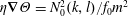
are both separately conserved. Following Bretherton & Garrett (Reference Bretherton and Garrett1968), the action in (3.1) is the wave energy divided by the intrinsic frequency; YBJ observed that to leading order the wave energy is only kinetic and the intrinsic frequency in (3.1) is the inertial frequency
 $f_{0}$
.
$f_{0}$
.
The conserved energy density
 ${\mathcal{E}}$
in (3.2) is the sum of the kinetic energy of the balanced flow,
${\mathcal{E}}$
in (3.2) is the sum of the kinetic energy of the balanced flow,
 $$\begin{eqnarray}\displaystyle & \displaystyle {\mathcal{K}}\,\stackrel{def}{=}\,{\textstyle \frac{1}{2}}|\unicode[STIX]{x1D735}\unicode[STIX]{x1D713}|^{2}, & \displaystyle\end{eqnarray}$$
and the potential energy of the near-inertial waves,
 $$\begin{eqnarray}\displaystyle & \displaystyle {\mathcal{P}}\,\stackrel{def}{=}\,{\textstyle \frac{1}{2}}b^{2}/N_{0}^{2}={\textstyle \frac{1}{4}}\unicode[STIX]{x1D706}^{2}|\unicode[STIX]{x1D735}\unicode[STIX]{x1D719}|^{2}. & \displaystyle\end{eqnarray}$$
Above,
 $b\propto \unicode[STIX]{x2202}\unicode[STIX]{x1D719}$
is the wave buoyancy defined in (2.4). We emphasize again that
$b\propto \unicode[STIX]{x2202}\unicode[STIX]{x1D719}$
is the wave buoyancy defined in (2.4). We emphasize again that
 $\unicode[STIX]{x1D713}$
is the streamfunction of the Lagrangian-mean flow, which is in geostrophic balance; the Eulerian-mean flow is not in balance. Thus we refer to
$\unicode[STIX]{x1D713}$
is the streamfunction of the Lagrangian-mean flow, which is in geostrophic balance; the Eulerian-mean flow is not in balance. Thus we refer to
 ${\mathcal{K}}$
as the kinetic energy of the balanced flow.
${\mathcal{K}}$
as the kinetic energy of the balanced flow.
XV explain the physical basis of stimulated generation by noting that balanced kinetic energy
 ${\mathcal{K}}$
can be converted into wave potential energy
${\mathcal{K}}$
can be converted into wave potential energy
 ${\mathcal{P}}$
while conserving the integral of the total energy
${\mathcal{P}}$
while conserving the integral of the total energy
 ${\mathcal{E}}$
in (3.2). Indeed, this conversion must occur if
${\mathcal{E}}$
in (3.2). Indeed, this conversion must occur if
 $\unicode[STIX]{x1D735}\unicode[STIX]{x1D719}$
is increased by a combination of refraction and advection in the wave equation (2.8). In the example shown in figure 1, the initial wave field in (2.14) has infinite spatial scale and therefore there is no wave potential energy at
$\unicode[STIX]{x1D735}\unicode[STIX]{x1D719}$
is increased by a combination of refraction and advection in the wave equation (2.8). In the example shown in figure 1, the initial wave field in (2.14) has infinite spatial scale and therefore there is no wave potential energy at
 $t=0$
. The subsequent evolution in figure 1 involves creation of non-zero
$t=0$
. The subsequent evolution in figure 1 involves creation of non-zero
 $\unicode[STIX]{x1D735}\unicode[STIX]{x1D719}$
, corresponding to gain of
$\unicode[STIX]{x1D735}\unicode[STIX]{x1D719}$
, corresponding to gain of
 ${\mathcal{P}}$
at the expense of
${\mathcal{P}}$
at the expense of
 ${\mathcal{K}}$
: this is stimulated generation of near-inertial waves.
${\mathcal{K}}$
: this is stimulated generation of near-inertial waves.
To substantiate this intuition, and diagnose results from our simulation of wave-modified two-dimensional turbulence, we develop the conservation laws corresponding to (3.1) and (3.2) in more detail.
3.1 Action conservation equation and action flux
Multiplying the wave equation (2.8) by
 $\unicode[STIX]{x1D719}^{\star }$
and adding to the complex conjugate, we obtain a conservation equation for action density,
$\unicode[STIX]{x1D719}^{\star }$
and adding to the complex conjugate, we obtain a conservation equation for action density,
 $$\begin{eqnarray}\displaystyle & \displaystyle \unicode[STIX]{x2202}_{t}{\mathcal{A}}+J(\unicode[STIX]{x1D713},{\mathcal{A}})+\unicode[STIX]{x1D735}\boldsymbol{\cdot }\boldsymbol{{\mathcal{F}}}=\underbrace{{\displaystyle \frac{1}{2f_{0}}}(\unicode[STIX]{x1D719}^{\star }D_{\unicode[STIX]{x1D719}}+\unicode[STIX]{x1D719}D_{\unicode[STIX]{x1D719}^{\star }})}_{\stackrel{def}{=}D_{{\mathcal{A}}}}, & \displaystyle\end{eqnarray}$$
where the flux of near-inertial wave action is
 $$\begin{eqnarray}\displaystyle & \displaystyle \boldsymbol{{\mathcal{F}}}\,\stackrel{def}{=}\,{\displaystyle \frac{\text{i}}{4}}\unicode[STIX]{x1D706}^{2}(\unicode[STIX]{x1D719}\unicode[STIX]{x1D735}\unicode[STIX]{x1D719}^{\star }-\unicode[STIX]{x1D719}^{\star }\unicode[STIX]{x1D735}\unicode[STIX]{x1D719}). & \displaystyle\end{eqnarray}$$
The local conservation law (3.5) shows how the wave action
 ${\mathcal{A}}$
changes due to geostrophic advection and divergence of the wave flux and dissipation – the second, third and fourth terms in (3.5).
${\mathcal{A}}$
changes due to geostrophic advection and divergence of the wave flux and dissipation – the second, third and fourth terms in (3.5).
The wave action flux
 $\boldsymbol{{\mathcal{F}}}$
is analogous to the probability current of quantum mechanics (e.g. Landau & Lifshitz Reference Landau and Lifshitz2013, p. 57). Using the polar representation
$\boldsymbol{{\mathcal{F}}}$
is analogous to the probability current of quantum mechanics (e.g. Landau & Lifshitz Reference Landau and Lifshitz2013, p. 57). Using the polar representation
 $\unicode[STIX]{x1D719}=|\unicode[STIX]{x1D719}|\text{e}^{\text{i}\unicode[STIX]{x1D6E9}}$
, the wave action flux
$\unicode[STIX]{x1D719}=|\unicode[STIX]{x1D719}|\text{e}^{\text{i}\unicode[STIX]{x1D6E9}}$
, the wave action flux
 $\boldsymbol{{\mathcal{F}}}$
can also be written as
$\boldsymbol{{\mathcal{F}}}$
can also be written as
 $$\begin{eqnarray}\displaystyle & \displaystyle \boldsymbol{{\mathcal{F}}}={\mathcal{A}}\,\unicode[STIX]{x1D702}\unicode[STIX]{x1D735}\unicode[STIX]{x1D6E9}, & \displaystyle\end{eqnarray}$$
where recall that
 $\unicode[STIX]{x1D702}=f_{0}\unicode[STIX]{x1D706}^{2}$
is the dispersivity. In (3.7),
$\unicode[STIX]{x1D702}=f_{0}\unicode[STIX]{x1D706}^{2}$
is the dispersivity. In (3.7),
 $\unicode[STIX]{x1D702}\unicode[STIX]{x1D735}\unicode[STIX]{x1D6E9}$
is the ‘generalized group velocity’ of hydrostatic near-inertial waves, i.e.
$\unicode[STIX]{x1D702}\unicode[STIX]{x1D735}\unicode[STIX]{x1D6E9}$
is the ‘generalized group velocity’ of hydrostatic near-inertial waves, i.e.
 $\boldsymbol{{\mathcal{F}}}$
is the generalized group velocity times the action density
$\boldsymbol{{\mathcal{F}}}$
is the generalized group velocity times the action density
 ${\mathcal{A}}$
. We use the term ‘generalized’ because no WKB-type (Wentzel–Kramers–Brillouin) scale separation is required to obtain the results above. The connection to standard internal-wave group velocity is quickly verified by considering a plane near-inertial wave with
${\mathcal{A}}$
. We use the term ‘generalized’ because no WKB-type (Wentzel–Kramers–Brillouin) scale separation is required to obtain the results above. The connection to standard internal-wave group velocity is quickly verified by considering a plane near-inertial wave with
 $\unicode[STIX]{x1D6E9}=kx+ly$
, yielding
$\unicode[STIX]{x1D6E9}=kx+ly$
, yielding
 $\unicode[STIX]{x1D702}\unicode[STIX]{x1D735}\unicode[STIX]{x1D6E9}=N_{0}^{2}(k,l)/f_{0}m^{2}$
.
$\unicode[STIX]{x1D702}\unicode[STIX]{x1D735}\unicode[STIX]{x1D6E9}=N_{0}^{2}(k,l)/f_{0}m^{2}$
.
Another useful identity involving the action flux
 $\boldsymbol{{\mathcal{F}}}$
is
$\boldsymbol{{\mathcal{F}}}$
is
 $$\begin{eqnarray}\displaystyle & \displaystyle \unicode[STIX]{x1D735}\boldsymbol{\cdot }(\hat{\boldsymbol{k}}\times \boldsymbol{{\mathcal{F}}})={\displaystyle \frac{\text{i}}{2}}\unicode[STIX]{x1D706}^{2}J(\unicode[STIX]{x1D719}^{\star },\unicode[STIX]{x1D719}), & \displaystyle\end{eqnarray}$$
where
 $\hat{\boldsymbol{k}}$
is the unit vector perpendicular to the
$\hat{\boldsymbol{k}}$
is the unit vector perpendicular to the
 $(x,y)$
-plane. Using (3.8), and the definition of action in (3.1), the wave PV
$(x,y)$
-plane. Using (3.8), and the definition of action in (3.1), the wave PV
 $q^{w}$
in (2.6) can be written as
$q^{w}$
in (2.6) can be written as
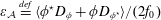
 $$\begin{eqnarray}\displaystyle & \displaystyle q^{w}={\textstyle \frac{1}{2}}\unicode[STIX]{x0394}{\mathcal{A}}+\unicode[STIX]{x1D702}^{-1}\unicode[STIX]{x1D735}\boldsymbol{\cdot }(\hat{\boldsymbol{k}}\times \boldsymbol{{\mathcal{F}}}). & \displaystyle\end{eqnarray}$$
Denoting an average over the domain by
 $\langle \rangle$
, and assuming that the action flux divergence
$\langle \rangle$
, and assuming that the action flux divergence
 $\unicode[STIX]{x1D735}\boldsymbol{\cdot }\boldsymbol{{\mathcal{F}}}$
vanishes after integration, we obtain from (3.5)
$\unicode[STIX]{x1D735}\boldsymbol{\cdot }\boldsymbol{{\mathcal{F}}}$
vanishes after integration, we obtain from (3.5)
 $$\begin{eqnarray}\displaystyle & \displaystyle {\displaystyle \frac{\text{d}\langle {\mathcal{A}}\rangle }{\text{d}t}}=\unicode[STIX]{x1D700}_{{\mathcal{A}}}, & \displaystyle\end{eqnarray}$$
where
 $\unicode[STIX]{x1D700}_{{\mathcal{A}}}\,\stackrel{def}{=}\,\langle \unicode[STIX]{x1D719}^{\star }D_{\unicode[STIX]{x1D719}}+\unicode[STIX]{x1D719}D_{\unicode[STIX]{x1D719}^{\star }}\rangle /(2f_{0})$
is the domain average of the dissipative term on the right of (3.5). In the example shown in figure 1 the total action
$\unicode[STIX]{x1D700}_{{\mathcal{A}}}\,\stackrel{def}{=}\,\langle \unicode[STIX]{x1D719}^{\star }D_{\unicode[STIX]{x1D719}}+\unicode[STIX]{x1D719}D_{\unicode[STIX]{x1D719}^{\star }}\rangle /(2f_{0})$
is the domain average of the dissipative term on the right of (3.5). In the example shown in figure 1 the total action
 $\langle {\mathcal{A}}\rangle$
is conserved to within 1 % over the course of the integration.
$\langle {\mathcal{A}}\rangle$
is conserved to within 1 % over the course of the integration.
3.2 Ehrenfest’s theorem
The quantum analogy suggests that we should seek an analogue of Ehrenfest’s theorem (the quantum equivalent of Newton’s law that force equals mass times acceleration). Thus in appendix B we develop a local conservation law for
 $\boldsymbol{{\mathcal{F}}}$
. The domain average of that result is
$\boldsymbol{{\mathcal{F}}}$
. The domain average of that result is
 $$\begin{eqnarray}\displaystyle & \displaystyle {\displaystyle \frac{\text{d}\langle \boldsymbol{{\mathcal{F}}}\rangle }{\text{d}t}}=\hat{\boldsymbol{k}}\times \langle \unicode[STIX]{x1D701}\,\boldsymbol{{\mathcal{F}}}\rangle -\hat{\boldsymbol{k}}\times \langle (\boldsymbol{{\mathcal{F}}}\boldsymbol{\cdot }\unicode[STIX]{x1D735})\unicode[STIX]{x1D735}\unicode[STIX]{x1D713}\rangle -\unicode[STIX]{x1D702}\left\langle {\mathcal{A}}\,\unicode[STIX]{x1D735}{\displaystyle \frac{1}{2}}\unicode[STIX]{x1D701}\right\rangle +\unicode[STIX]{x1D73A}_{\boldsymbol{{\mathcal{F}}}}. & \displaystyle\end{eqnarray}$$
In the quantum analogy,
 $\boldsymbol{{\mathcal{F}}}$
is momentum and the left-hand side of (3.11) is mass times acceleration; the forces are on the right of (3.11). Starting from the end,
$\boldsymbol{{\mathcal{F}}}$
is momentum and the left-hand side of (3.11) is mass times acceleration; the forces are on the right of (3.11). Starting from the end,
 $\unicode[STIX]{x1D73A}_{\boldsymbol{{\mathcal{F}}}}$
is a dissipative term defined in appendix B. The third term on the right of (3.11) is the force due to the gradient of the potential
$\unicode[STIX]{x1D73A}_{\boldsymbol{{\mathcal{F}}}}$
is a dissipative term defined in appendix B. The third term on the right of (3.11) is the force due to the gradient of the potential
 $\unicode[STIX]{x1D701}/2$
. The second term on the right of (3.11) represents the combined effect of stretching and tilting of
$\unicode[STIX]{x1D701}/2$
. The second term on the right of (3.11) represents the combined effect of stretching and tilting of
 $\boldsymbol{{\mathcal{F}}}$
by the geostrophic flow. The first term on the right of (3.11) is a ‘vortex force’, again due to
$\boldsymbol{{\mathcal{F}}}$
by the geostrophic flow. The first term on the right of (3.11) is a ‘vortex force’, again due to
 $\unicode[STIX]{x1D701}$
, but perpendicular to
$\unicode[STIX]{x1D701}$
, but perpendicular to
 $\boldsymbol{{\mathcal{F}}}$
. The two
$\boldsymbol{{\mathcal{F}}}$
. The two
 $\hat{\boldsymbol{k}}\times$
terms on the right lack quantum analogues.
$\hat{\boldsymbol{k}}\times$
terms on the right lack quantum analogues.
The results in this section are obtained from the wave equation (2.8) without using the PV equation (2.7). In other words, (3.5)–(3.11) apply to the YBJ equation with
 $\text{e}^{\text{i}mz}$
structure regardless of the balanced flow dynamics. We turn now to energy conservation and consideration of the PV equation (2.7).
$\text{e}^{\text{i}mz}$
structure regardless of the balanced flow dynamics. We turn now to energy conservation and consideration of the PV equation (2.7).
3.3 Energy conservation and conversion
The energy conservation law is considerably more complicated than action conservation. We sequester the details of the local conservation laws to appendix B and present here the simpler results obtained by domain averaging those local conservation laws. The results in (3.12) through (3.16) below are obtained by: (i) multiplying the wave equation (2.8) by
 $\unicode[STIX]{x0394}\unicode[STIX]{x1D719}^{\star }$
, forming the average
$\unicode[STIX]{x0394}\unicode[STIX]{x1D719}^{\star }$
, forming the average
 $\langle \rangle$
and adding the complex conjugate; and by (ii) multiplying the PV equation (2.7) by
$\langle \rangle$
and adding the complex conjugate; and by (ii) multiplying the PV equation (2.7) by
 $-\unicode[STIX]{x1D713}$
and averaging
$-\unicode[STIX]{x1D713}$
and averaging
 $\langle \rangle$
.
$\langle \rangle$
.
For the wave potential energy in (3.4) and the balanced kinetic energy in (3.3) we find
 $$\begin{eqnarray}\displaystyle & \displaystyle {\displaystyle \frac{\text{d}\langle {\mathcal{P}}\rangle }{\text{d}t}}=\unicode[STIX]{x1D6E4}_{r}+\unicode[STIX]{x1D6E4}_{a}+\unicode[STIX]{x1D700}_{{\mathcal{P}}}, & \displaystyle\end{eqnarray}$$
 $$\begin{eqnarray}\displaystyle & \displaystyle {\displaystyle \frac{\text{d}\langle {\mathcal{K}}\rangle }{\text{d}t}}=-\unicode[STIX]{x1D6E4}_{r}-\unicode[STIX]{x1D6E4}_{a}+\unicode[STIX]{x1D6EF}+\unicode[STIX]{x1D700}_{{\mathcal{K}}}, & \displaystyle\end{eqnarray}$$
where the ‘conversion terms’ in (3.12) and (3.13) are
 $$\begin{eqnarray}\displaystyle & \displaystyle \unicode[STIX]{x1D6E4}_{r}\,\stackrel{def}{=}\,\left\langle {\textstyle \frac{1}{2}}\unicode[STIX]{x1D701}\,\unicode[STIX]{x1D735}\boldsymbol{\cdot }\boldsymbol{{\mathcal{F}}}\right\rangle , & \displaystyle\end{eqnarray}$$
and
 $$\begin{eqnarray}\displaystyle \displaystyle \unicode[STIX]{x1D6E4}_{a}~\stackrel{def}{=}~{\displaystyle \frac{\unicode[STIX]{x1D706}^{2}}{4}}\langle \unicode[STIX]{x0394}\unicode[STIX]{x1D719}^{\star }J(\unicode[STIX]{x1D713},\unicode[STIX]{x1D719})+\unicode[STIX]{x0394}\unicode[STIX]{x1D719}J(\unicode[STIX]{x1D713},\unicode[STIX]{x1D719}^{\star })\rangle & & \displaystyle\end{eqnarray}$$

The dissipative terms,
 $\unicode[STIX]{x1D700}_{{\mathcal{P}}}$
,
$\unicode[STIX]{x1D700}_{{\mathcal{P}}}$
,
 $\unicode[STIX]{x1D700}_{{\mathcal{K}}}$
and
$\unicode[STIX]{x1D700}_{{\mathcal{K}}}$
and
 $\unicode[STIX]{x1D6EF}$
are defined in appendix B.
$\unicode[STIX]{x1D6EF}$
are defined in appendix B.
 $\unicode[STIX]{x1D6EF}$
in (3.13) is particularly interesting: dissipation of waves
$\unicode[STIX]{x1D6EF}$
in (3.13) is particularly interesting: dissipation of waves
 $D_{\unicode[STIX]{x1D719}}$
produces balanced kinetic energy. Summing (3.12) and (3.13) the ‘conversion’ terms
$D_{\unicode[STIX]{x1D719}}$
produces balanced kinetic energy. Summing (3.12) and (3.13) the ‘conversion’ terms
 $\unicode[STIX]{x1D6E4}_{r}$
and
$\unicode[STIX]{x1D6E4}_{r}$
and
 $\unicode[STIX]{x1D6E4}_{a}$
cancel, and we obtain the conservation law for total energy
$\unicode[STIX]{x1D6E4}_{a}$
cancel, and we obtain the conservation law for total energy
 $\langle {\mathcal{E}}\rangle =\langle {\mathcal{P}}+{\mathcal{K}}\rangle$
.
$\langle {\mathcal{E}}\rangle =\langle {\mathcal{P}}+{\mathcal{K}}\rangle$
.

Figure 3. Illustration of energy conversion terms in the Lamb–Chaplygin dipole solution with parameters presented in table 2. (a) The action flux
 $\boldsymbol{{\mathcal{F}}}$
overlaid on contours of relative vorticity
$\boldsymbol{{\mathcal{F}}}$
overlaid on contours of relative vorticity
 $\unicode[STIX]{x0394}\unicode[STIX]{x1D713}/(U_{e}k_{e})=[-1.5,-0.5,0.5,1.5]$
, with dashed lines showing negative values; the scale of the action flux is
$\unicode[STIX]{x0394}\unicode[STIX]{x1D713}/(U_{e}k_{e})=[-1.5,-0.5,0.5,1.5]$
, with dashed lines showing negative values; the scale of the action flux is
 $F=f_{0}\unicode[STIX]{x1D706}^{2}k_{e}U_{w}^{2}$
. (b) The local advective conversion (i.e. the non-averaged
$F=f_{0}\unicode[STIX]{x1D706}^{2}k_{e}U_{w}^{2}$
. (b) The local advective conversion (i.e. the non-averaged
 $\unicode[STIX]{x1D6E4}_{a}$
) overlaid on contours of streamfunction
$\unicode[STIX]{x1D6E4}_{a}$
) overlaid on contours of streamfunction
 $\unicode[STIX]{x1D713}\times (U_{e}/k_{e})=[-8,-4,-2,0,2,4,8]$
.
$\unicode[STIX]{x1D713}\times (U_{e}/k_{e})=[-8,-4,-2,0,2,4,8]$
.
The refractive conversion
 $\unicode[STIX]{x1D6E4}_{r}$
stems from
$\unicode[STIX]{x1D6E4}_{r}$
stems from
 $\text{i}\unicode[STIX]{x1D719}\unicode[STIX]{x1D701}/2$
in the wave equation and is easy to interpret: the convergence of the wave action flux,
$\text{i}\unicode[STIX]{x1D719}\unicode[STIX]{x1D701}/2$
in the wave equation and is easy to interpret: the convergence of the wave action flux,
 $\unicode[STIX]{x1D735}\boldsymbol{\cdot }\boldsymbol{{\mathcal{F}}}<0$
, into anti-cyclones,
$\unicode[STIX]{x1D735}\boldsymbol{\cdot }\boldsymbol{{\mathcal{F}}}<0$
, into anti-cyclones,
 $\unicode[STIX]{x1D701}<0$
, is a source of wave potential energy
$\unicode[STIX]{x1D701}<0$
, is a source of wave potential energy
 ${\mathcal{P}}$
; similarly, the divergence of the wave action flux from cyclones is a source of
${\mathcal{P}}$
; similarly, the divergence of the wave action flux from cyclones is a source of
 ${\mathcal{P}}$
. Figure 3(a) shows the convergence of
${\mathcal{P}}$
. Figure 3(a) shows the convergence of
 $\boldsymbol{{\mathcal{F}}}$
into the anti-cyclone (and divergence from the cyclone) of the dipole solution at
$\boldsymbol{{\mathcal{F}}}$
into the anti-cyclone (and divergence from the cyclone) of the dipole solution at
 $t\times U_{e}k_{e}=1$
, which yields the sharp initial increase of
$t\times U_{e}k_{e}=1$
, which yields the sharp initial increase of
 $\langle {\mathcal{P}}\rangle$
discussed below. Ehrenfest’s theorem in (3.11) illuminates the initial structure of
$\langle {\mathcal{P}}\rangle$
discussed below. Ehrenfest’s theorem in (3.11) illuminates the initial structure of
 $\boldsymbol{{\mathcal{F}}}$
in figure 3. Because
$\boldsymbol{{\mathcal{F}}}$
in figure 3. Because
 $\unicode[STIX]{x1D719}$
is initially uniform, the initial tendency of
$\unicode[STIX]{x1D719}$
is initially uniform, the initial tendency of
 $\boldsymbol{{\mathcal{F}}}$
is
$\boldsymbol{{\mathcal{F}}}$
is
 $$\begin{eqnarray}\displaystyle & \displaystyle \unicode[STIX]{x2202}_{t}\boldsymbol{{\mathcal{F}}}(0)=-\unicode[STIX]{x1D702}{\mathcal{A}}\unicode[STIX]{x1D735}{\textstyle \frac{1}{2}}\unicode[STIX]{x1D701}. & \displaystyle\end{eqnarray}$$
Thus the action flux is initially anti-parallel to the gradient of relative vorticity (see figure 3 a), and wave action converges into anti-cyclones (and diverges from cyclones).

The advective conversion
 $\unicode[STIX]{x1D6E4}_{a}$
in (3.12) and (3.13) stems from the term
$\unicode[STIX]{x1D6E4}_{a}$
in (3.12) and (3.13) stems from the term
 $J(\unicode[STIX]{x1D713},\unicode[STIX]{x1D719})$
in the wave equation (2.8) and is a source of
$J(\unicode[STIX]{x1D713},\unicode[STIX]{x1D719})$
in the wave equation (2.8) and is a source of
 $\langle {\mathcal{P}}\rangle$
due to straining and deformation of the wave field by the geostrophic flow. The symmetric
$\langle {\mathcal{P}}\rangle$
due to straining and deformation of the wave field by the geostrophic flow. The symmetric
 $2\times 2$
matrix in (3.16) is the strain or deformation tensor of the geostrophic flow. Thus, in analogy with passive-scalar gradient amplification, straining also enhances gradients of the back-rotated near-inertial velocity
$2\times 2$
matrix in (3.16) is the strain or deformation tensor of the geostrophic flow. Thus, in analogy with passive-scalar gradient amplification, straining also enhances gradients of the back-rotated near-inertial velocity
 $\unicode[STIX]{x1D719}$
, thereby generating wave potential energy
$\unicode[STIX]{x1D719}$
, thereby generating wave potential energy
 $\langle {\mathcal{P}}\rangle$
.
$\langle {\mathcal{P}}\rangle$
.
3.4 Energetics of the Lamb–Chaplygin dipole solution
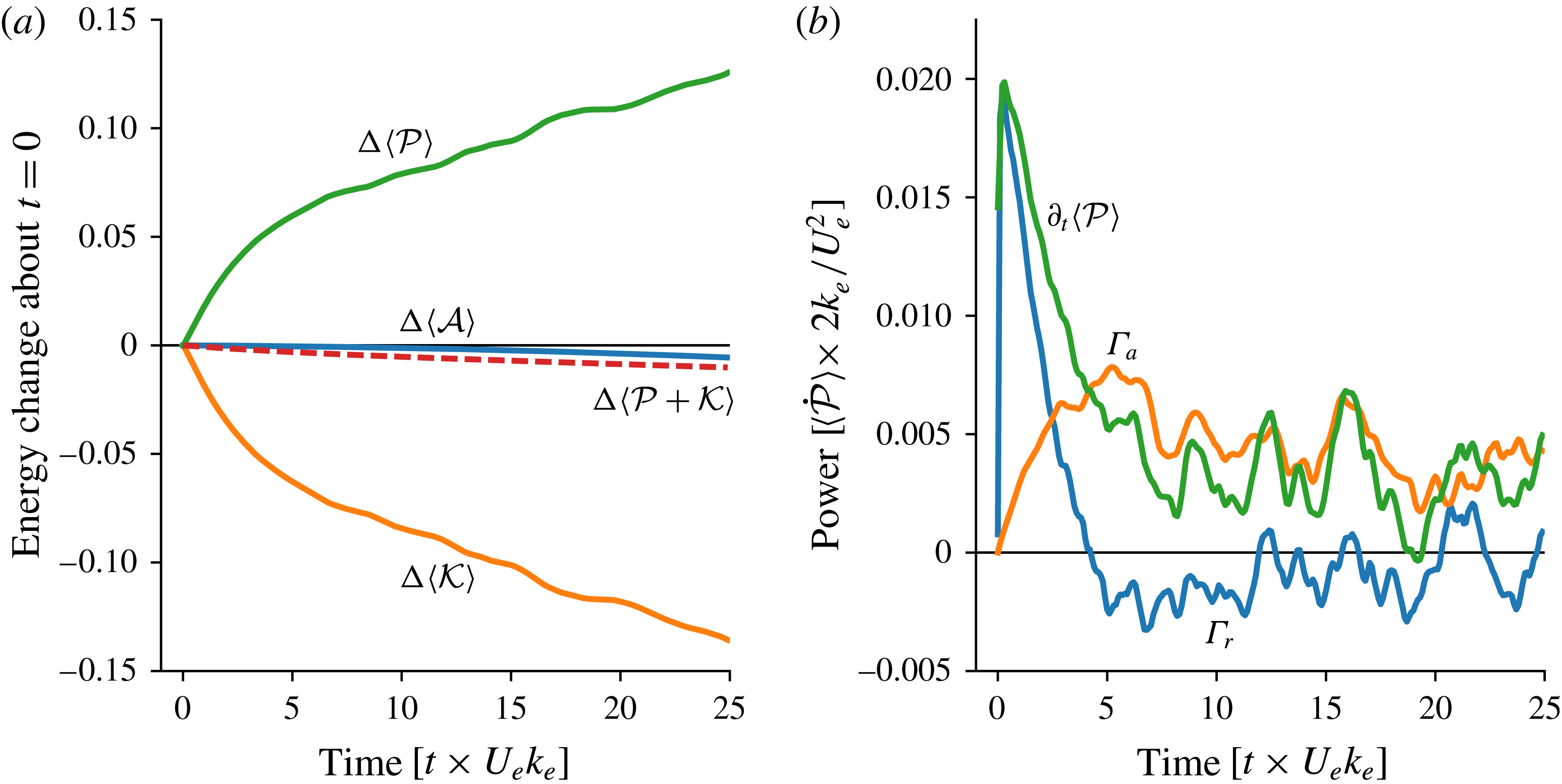
Figure 4 shows the energetics of the Lamb–Chaplygin dipole solution in figure 1. In figure 4(a),
 ${\mathcal{P}}$
increases at the expense of
${\mathcal{P}}$
increases at the expense of
 ${\mathcal{K}}$
, while
${\mathcal{K}}$
, while
 ${\mathcal{A}}$
is conserved. The wave potential energy budget in figure 4(b) shows that this stimulated generation occurs in two stages. First, refraction of the initially uniform wave field causes a dramatic concentration of waves into the anti-cyclone, producing a sharp increase
${\mathcal{A}}$
is conserved. The wave potential energy budget in figure 4(b) shows that this stimulated generation occurs in two stages. First, refraction of the initially uniform wave field causes a dramatic concentration of waves into the anti-cyclone, producing a sharp increase
 ${\mathcal{P}}$
through
${\mathcal{P}}$
through
 $\unicode[STIX]{x1D6E4}_{r}$
. But this rapid initial energy conversion does not last long because the wave feedback deforms the anti-cyclone and dispersion radiates waves away from the dipole (see figure 1). Thus in figure 4(b),
$\unicode[STIX]{x1D6E4}_{r}$
. But this rapid initial energy conversion does not last long because the wave feedback deforms the anti-cyclone and dispersion radiates waves away from the dipole (see figure 1). Thus in figure 4(b),
 $\unicode[STIX]{x1D6E4}_{r}$
decreases sharply, and eventually reverses sign at
$\unicode[STIX]{x1D6E4}_{r}$
decreases sharply, and eventually reverses sign at
 $t\times U_{e}k_{e}\approx 8$
.
$t\times U_{e}k_{e}\approx 8$
.
The second stage of stimulated generation starts after refraction has created dipole-scale waves. Advection by the balanced flow can then strain the waves, further reducing their lateral scale (figure 4
b). The ensuing advective conversion,
 $\unicode[STIX]{x1D6E4}_{a}$
, starts at
$\unicode[STIX]{x1D6E4}_{a}$
, starts at
 $t\times U_{e}k_{e}\approx 4$
. Straining by the balanced flow sustains this advective generation of
$t\times U_{e}k_{e}\approx 4$
. Straining by the balanced flow sustains this advective generation of
 ${\mathcal{P}}$
. The waves eventually escape the straining regions through dispersion and the conversion nearly halts at
${\mathcal{P}}$
. The waves eventually escape the straining regions through dispersion and the conversion nearly halts at
 $t\times U_{e}k_{e}=30$
. The time-integrated
$t\times U_{e}k_{e}=30$
. The time-integrated
 $\unicode[STIX]{x1D6E4}_{a}$
accounts for
$\unicode[STIX]{x1D6E4}_{a}$
accounts for
 ${\approx}78\,\%$
of the wave potential energy generation; table 3 summarizes the energy budget.
${\approx}78\,\%$
of the wave potential energy generation; table 3 summarizes the energy budget.
Table 3. The time-integrated budget of wave potential energy and quasi-geostrophic kinetic energy of the Lamb–Chaplygin dipole solutions with parameters provided in table 2. The energy budgets close within
 $10^{-6}\,\%$
.
$10^{-6}\,\%$
.

3.5 Summary
The expressions for energy conversion in (3.14) and (3.16) clarify the mechanism of stimulated generation triggered by the initially uniform near-inertial wave in (2.14). First, refraction causes a convergence of wave action into anti-cyclones. Then advection strains the waves, reducing their lateral scale. Both processes amplify the lateral gradients of wave amplitude, thereby generating wave potential energy
 ${\mathcal{P}}$
at the expense of balanced kinetic energy
${\mathcal{P}}$
at the expense of balanced kinetic energy
 ${\mathcal{K}}$
. Wave action
${\mathcal{K}}$
. Wave action
 ${\mathcal{A}}$
is conserved throughout this process.
${\mathcal{A}}$
is conserved throughout this process.
In the remainder of this paper, we describe and quantify stimulated generation in an idealization of an oceanographic post-storm scenario: the uniform initial near-inertial wave in (2.14) interacts with two-dimensional turbulence.
4 Two-dimensional turbulence modified by near-inertial waves
To study the energy exchange between near-inertial waves and geostrophic flow in a turbulent regime, we consider a barotropic flow that emerges from random initial conditions integrated for 20 eddy turnover time units. In other words, we first integrate the initial condition
 $$\begin{eqnarray}\displaystyle & \displaystyle \unicode[STIX]{x1D713}(x,y,t\times U_{e}k_{e}=-20)=\mathop{\sum }_{k,l}\unicode[STIX]{x1D713}_{\boldsymbol{k}}\cos (kx+ly+\unicode[STIX]{x1D712}_{\boldsymbol{k}}) & \displaystyle\end{eqnarray}$$
with waveless QG dynamics before introducing the wave in (2.14) at
 $t\times U_{e}k_{e}=0$
. Above,
$t\times U_{e}k_{e}=0$
. Above,
 $\unicode[STIX]{x1D712}_{\boldsymbol{k}}$
is a random phase uniformly distributed on
$\unicode[STIX]{x1D712}_{\boldsymbol{k}}$
is a random phase uniformly distributed on
 $[0,2\unicode[STIX]{x03C0})$
, and
$[0,2\unicode[STIX]{x03C0})$
, and
 $\unicode[STIX]{x1D713}_{\boldsymbol{k}}$
is the streamfunction isotropic spectrum
$\unicode[STIX]{x1D713}_{\boldsymbol{k}}$
is the streamfunction isotropic spectrum
 $$\begin{eqnarray}\displaystyle & \displaystyle \unicode[STIX]{x1D713}_{\boldsymbol{k}}=C\times \{|\boldsymbol{k}|\,[1+(|\boldsymbol{k}|/k_{e})^{4}]\}^{-1/2}, & \displaystyle\end{eqnarray}$$
with the wavenumber magnitude
 $|\boldsymbol{k}|^{2}=k^{2}+l^{2}$
. The prescribed initial energy
$|\boldsymbol{k}|^{2}=k^{2}+l^{2}$
. The prescribed initial energy
 $U_{e}^{2}/2$
determines the constant
$U_{e}^{2}/2$
determines the constant
 $C$
:
$C$
:
 $$\begin{eqnarray}\displaystyle & \displaystyle \mathop{\sum }_{k,l}\underbrace{|\boldsymbol{k}|^{2}{\unicode[STIX]{x1D713}_{\boldsymbol{k}}}^{2}}_{\stackrel{def}{=}{\mathcal{K}}_{e}}={\textstyle \frac{1}{2}}U_{e}^{2}. & \displaystyle\end{eqnarray}$$
The kinetic energy spectrum,
 ${\mathcal{K}}_{e}$
, peaks at the energy-containing scale
${\mathcal{K}}_{e}$
, peaks at the energy-containing scale
 $k_{e}^{-1}$
. At scales larger than
$k_{e}^{-1}$
. At scales larger than
 $k_{e}^{-1}$
,
$k_{e}^{-1}$
,
 ${\mathcal{K}}_{e}$
has a linear dependence on
${\mathcal{K}}_{e}$
has a linear dependence on
 $|\boldsymbol{k}|$
, whereas
$|\boldsymbol{k}|$
, whereas
 ${\mathcal{K}}_{e}$
decays as
${\mathcal{K}}_{e}$
decays as
 $|\boldsymbol{k}|^{-3}$
at scales smaller than
$|\boldsymbol{k}|^{-3}$
at scales smaller than
 $k_{e}^{-1}$
. This red spectrum ensures insignificant loss of energy by small-scale dissipation
$k_{e}^{-1}$
. This red spectrum ensures insignificant loss of energy by small-scale dissipation
 $D_{q}$
in (2.7). Over the course of the simulations described below, the centroid wavenumber of the balanced kinetic energy spectrum decreases by
$D_{q}$
in (2.7). Over the course of the simulations described below, the centroid wavenumber of the balanced kinetic energy spectrum decreases by
 $50\,\%$
;
$50\,\%$
;
 $k_{e}^{-1}$
is thus a reasonable scale to characterize the size of the balanced flow throughout the evolution.
$k_{e}^{-1}$
is thus a reasonable scale to characterize the size of the balanced flow throughout the evolution.
In the case with no waves, that is
 $q^{w}=0$
, the PV equation (2.7) reduces to two-dimensional (2-D) fluid mechanics and the quasi-inviscid evolution of a random initial condition is the well-studied problem of 2-D turbulence. Stirring of vorticity
$q^{w}=0$
, the PV equation (2.7) reduces to two-dimensional (2-D) fluid mechanics and the quasi-inviscid evolution of a random initial condition is the well-studied problem of 2-D turbulence. Stirring of vorticity
 $\unicode[STIX]{x0394}\unicode[STIX]{x1D713}$
transfers enstrophy towards small scales; energy flows to large scales. Most of enstrophy is dissipated within few eddy turnover times, whereas kinetic energy is nearly conserved. Vorticity concentrates into localized coherent structures: after 20 eddy turnover time units, the vorticity is well organized into an ensemble of vortices that form via like-sign vortex merging (e.g. Fornberg Reference Fornberg1977; McWilliams Reference McWilliams1984).
$\unicode[STIX]{x0394}\unicode[STIX]{x1D713}$
transfers enstrophy towards small scales; energy flows to large scales. Most of enstrophy is dissipated within few eddy turnover times, whereas kinetic energy is nearly conserved. Vorticity concentrates into localized coherent structures: after 20 eddy turnover time units, the vorticity is well organized into an ensemble of vortices that form via like-sign vortex merging (e.g. Fornberg Reference Fornberg1977; McWilliams Reference McWilliams1984).
4.1 Relevant parameters
The scaling
 $$\begin{eqnarray}\displaystyle & \displaystyle \text{length}\sim k_{e}^{^{-1}},\quad \text{time}\sim (U_{e}k_{e})^{-1},\quad \unicode[STIX]{x1D713}\sim U_{e}k_{e}^{-1},\quad \text{and}\quad \unicode[STIX]{x1D719}\sim U_{w}, & \displaystyle\end{eqnarray}$$
shows that there are two important dimensionless control parameters. The first is
 $$\begin{eqnarray}\displaystyle & \displaystyle \unicode[STIX]{x1D6FC}\,\stackrel{def}{=}\,\underbrace{{\displaystyle \frac{U_{e}k_{e}}{f_{0}}}}_{\stackrel{def}{=}Ro}\times \left({\displaystyle \frac{U_{w}}{U_{e}}}\right)^{2}, & \displaystyle\end{eqnarray}$$
which scales the contribution of the wave terms in the potential vorticity (2.6). The second dimensionless parameter is
 $$\begin{eqnarray}\displaystyle & \displaystyle \hslash \,\stackrel{def}{=}\,\unicode[STIX]{x1D702}\times {\displaystyle \frac{k_{e}}{U_{e}}}=Ro^{-1}\times (\unicode[STIX]{x1D706}k_{e})^{2}, & \displaystyle\end{eqnarray}$$
which scales wave dispersion against the effects of advection and refraction. Assuming that the wave horizontal scale is
 $k_{e}^{-1}$
,
$k_{e}^{-1}$
,
 $(\unicode[STIX]{x1D706}k_{e})^{2}$
is the wave Burger number, which is small for near-inertial waves.
$(\unicode[STIX]{x1D706}k_{e})^{2}$
is the wave Burger number, which is small for near-inertial waves.
Table 4. Description of parameters of the 2-D turbulence simulations. The initial conditions are Rossby number
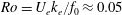 $Ro=U_{e}k_{e}/f_{0}\approx 0.05$
, wave dispersivity
$Ro=U_{e}k_{e}/f_{0}\approx 0.05$
, wave dispersivity
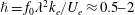 $\hslash =f_{0}\unicode[STIX]{x1D706}^{2}k_{e}/U_{e}\approx 0.5{-}2$
and wave amplitude
$\hslash =f_{0}\unicode[STIX]{x1D706}^{2}k_{e}/U_{e}\approx 0.5{-}2$
and wave amplitude
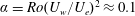 $\unicode[STIX]{x1D6FC}=Ro(U_{w}/U_{e})^{2}\approx 0.1$
.
$\unicode[STIX]{x1D6FC}=Ro(U_{w}/U_{e})^{2}\approx 0.1$
.


Figure 5. Snapshots of the turbulence solution with parameters in table 4. (a–c) PV
 $q$
. (d–f) Wave kinetic energy density
$q$
. (d–f) Wave kinetic energy density
 $|\unicode[STIX]{x1D719}|^{2}$
. (g–i) Wave buoyancy, with scale
$|\unicode[STIX]{x1D719}|^{2}$
. (g–i) Wave buoyancy, with scale
 $B=k_{e}mU_{w}f_{0}\unicode[STIX]{x1D706}^{2}$
. These plots show
$B=k_{e}mU_{w}f_{0}\unicode[STIX]{x1D706}^{2}$
. These plots show
 $(1/2)^{2}$
of the domain.
$(1/2)^{2}$
of the domain.

4.2 Solution with
 $\hslash =1$
and
$\unicode[STIX]{x1D6FC}=0.1$
$\hslash =1$
and
$\unicode[STIX]{x1D6FC}=0.1$


Figure 5 shows snapshots of a solution with
 $\hslash =1$
and
$\hslash =1$
and
 $\unicode[STIX]{x1D6FC}=0.1$
with further parameters in table 4. This turbulence solution shares qualitative aspects of the Lamb–Chaplygin solution. Starting from a uniform wave field in (2.14), refraction quickly concentrates the waves into anti-cyclones. Initially the action density
$\unicode[STIX]{x1D6FC}=0.1$
with further parameters in table 4. This turbulence solution shares qualitative aspects of the Lamb–Chaplygin solution. Starting from a uniform wave field in (2.14), refraction quickly concentrates the waves into anti-cyclones. Initially the action density
 ${\mathcal{A}}$
is uniform but by
${\mathcal{A}}$
is uniform but by
 $t\times U_{e}k_{e}\approx 1$
,
$t\times U_{e}k_{e}\approx 1$
,
 ${\mathcal{A}}$
varies on eddy scales by a factor of two with significant focusing of waves, indicated by maxima of
${\mathcal{A}}$
varies on eddy scales by a factor of two with significant focusing of waves, indicated by maxima of
 ${\mathcal{A}}$
, into anti-cyclones (compare (d–f) and (g–i) of figure 5).
${\mathcal{A}}$
, into anti-cyclones (compare (d–f) and (g–i) of figure 5).
Dispersion radiates waves from the vortices; advection enhances the gradients of back-rotated velocity
 $\unicode[STIX]{x1D719}$
(see figure 5
g–i, which depicts wave buoyancy). By
$\unicode[STIX]{x1D719}$
(see figure 5
g–i, which depicts wave buoyancy). By
 $t\times U_{e}k_{e}\approx 10$
,
$t\times U_{e}k_{e}\approx 10$
,
 ${\mathcal{A}}$
varies by a factor of five and the wave buoyancy is amplified by a factor of two. The evolution of potential vorticity
${\mathcal{A}}$
varies by a factor of five and the wave buoyancy is amplified by a factor of two. The evolution of potential vorticity
 $q$
is similar to that in the waveless problem: like-sign vortices merge into bigger vortices. The big vortices keep straining the waves, generating smaller scales in the wave field.
$q$
is similar to that in the waveless problem: like-sign vortices merge into bigger vortices. The big vortices keep straining the waves, generating smaller scales in the wave field.
Figure 6(a) shows the inexorable increase in wave potential energy
 $\langle {\mathcal{P}}\rangle$
and the corresponding decrease in balanced kinetic energy
$\langle {\mathcal{P}}\rangle$
and the corresponding decrease in balanced kinetic energy
 $\langle {\mathcal{K}}\rangle$
. In figure 6(b) quick wave refraction results in an initial sharp generation of
$\langle {\mathcal{K}}\rangle$
. In figure 6(b) quick wave refraction results in an initial sharp generation of
 $\langle {\mathcal{P}}\rangle$
at the expense of balanced kinetic energy
$\langle {\mathcal{P}}\rangle$
at the expense of balanced kinetic energy
 $\langle {\mathcal{K}}\rangle$
. As in the Lamb–Chaplygin solution, the positive refractive conversion,
$\langle {\mathcal{K}}\rangle$
. As in the Lamb–Chaplygin solution, the positive refractive conversion,
 $\unicode[STIX]{x1D6E4}_{r}>0$
, is ephemeral: in figure 6(b),
$\unicode[STIX]{x1D6E4}_{r}>0$
, is ephemeral: in figure 6(b),
 $\unicode[STIX]{x1D6E4}_{r}$
peaks at
$\unicode[STIX]{x1D6E4}_{r}$
peaks at
 $t\times U_{e}k_{e}\approx 2$
and then decays rapidly, eventually changing sign at
$t\times U_{e}k_{e}\approx 2$
and then decays rapidly, eventually changing sign at
 $t\times U_{e}k_{e}\approx 5$
. However, a significant positive advective conversion,
$t\times U_{e}k_{e}\approx 5$
. However, a significant positive advective conversion,
 $\unicode[STIX]{x1D6E4}_{a}>0$
, sustains stimulated generation so that
$\unicode[STIX]{x1D6E4}_{a}>0$
, sustains stimulated generation so that
 $\langle {\mathcal{P}}\rangle$
ultimately increases approximately linearly with time.
$\langle {\mathcal{P}}\rangle$
ultimately increases approximately linearly with time.
After 25 eddy turnover time units, the balanced kinetic energy
 $\langle {\mathcal{K}}\rangle$
has decayed by approximately
$\langle {\mathcal{K}}\rangle$
has decayed by approximately
 $14\,\%$
from its initial value. Most of this loss is by stimulated generation of
$14\,\%$
from its initial value. Most of this loss is by stimulated generation of
 $\langle {\mathcal{P}}\rangle$
. As in the Lamb–Chaplygin solution, advective conversion
$\langle {\mathcal{P}}\rangle$
. As in the Lamb–Chaplygin solution, advective conversion
 $\unicode[STIX]{x1D6E4}_{a}$
accounts for most of the energy change. Table 5 presents further details of the energy budget.
$\unicode[STIX]{x1D6E4}_{a}$
accounts for most of the energy change. Table 5 presents further details of the energy budget.
The solution illustrates interesting characteristics of stimulated generation. First, the role of refraction is catalytic in that it generates the initial eddy-scale gradients in
 $\unicode[STIX]{x1D719}$
that are then enhanced by advective straining; the advective conversion,
$\unicode[STIX]{x1D719}$
that are then enhanced by advective straining; the advective conversion,
 $\unicode[STIX]{x1D6E4}_{a}$
in (3.16), ultimately accounts for most of the energy transfer from turbulence to waves. Second, the approximately linear-in-time growth of wave potential energy
$\unicode[STIX]{x1D6E4}_{a}$
in (3.16), ultimately accounts for most of the energy transfer from turbulence to waves. Second, the approximately linear-in-time growth of wave potential energy
 $\langle {\mathcal{P}}\rangle$
is very slow in comparison with exponential increase of passive-scalar tracer gradients in turbulent velocity fields. The relatively slow growth of
$\langle {\mathcal{P}}\rangle$
is very slow in comparison with exponential increase of passive-scalar tracer gradients in turbulent velocity fields. The relatively slow growth of
 $\langle {\mathcal{P}}\rangle$
suggests that wave dispersion plays an important role in slowing and perhaps opposing advective straining (see § 5 for further discussion of dispersion and ‘wave escape’). To investigate whether these characteristics are general we consider solutions with varying vertical wavelengths and therefore different dispersivities.
$\langle {\mathcal{P}}\rangle$
suggests that wave dispersion plays an important role in slowing and perhaps opposing advective straining (see § 5 for further discussion of dispersion and ‘wave escape’). To investigate whether these characteristics are general we consider solutions with varying vertical wavelengths and therefore different dispersivities.
Table 5. The time-integrated budget of wave potential energy and QG kinetic energy of the reference 2-D turbulence solution with parameters in 4. The energy budgets close within
 $0.1\,\%$
.
$0.1\,\%$
.


Figure 7. Snapshots of PV
 $q$
and its decomposition into relative vorticity
$q$
and its decomposition into relative vorticity
 $\unicode[STIX]{x1D701}=\unicode[STIX]{x0394}\unicode[STIX]{x1D713}$
, and wave potential vorticity
$\unicode[STIX]{x1D701}=\unicode[STIX]{x0394}\unicode[STIX]{x1D713}$
, and wave potential vorticity
 $q^{w}$
. The snapshots were taken at
$q^{w}$
. The snapshots were taken at
 $t\times U_{e}k_{e}=25$
.
$t\times U_{e}k_{e}=25$
.

Figure 8. The energetics of 2-D turbulence solutions with different dispersivities. (a) Energy change about the initial condition. (b) The energy conversion terms in (3.12). (c) The correlation between relative vorticity and wave kinetic energy. (d) The skewness of relative vorticity.
4.3 Varying dispersivity
Figure 7 shows snapshots of potential vorticity
 $q$
and its constituents in a set of solutions with varying the vertical wavelength
$q$
and its constituents in a set of solutions with varying the vertical wavelength
 $2\unicode[STIX]{x03C0}\,m^{-1}$
from 280 m to 560 m, yielding dispersivities ranging from 0.5 to 2. (All other parameters are fixed.) The potential vorticity
$2\unicode[STIX]{x03C0}\,m^{-1}$
from 280 m to 560 m, yielding dispersivities ranging from 0.5 to 2. (All other parameters are fixed.) The potential vorticity
 $q$
shows more small-scale filamentation with decreasing dispersivity, but it is otherwise similar across the three solutions. The partition into relative vorticity
$q$
shows more small-scale filamentation with decreasing dispersivity, but it is otherwise similar across the three solutions. The partition into relative vorticity
 $\unicode[STIX]{x0394}\unicode[STIX]{x1D713}$
and wave potential vorticity
$\unicode[STIX]{x0394}\unicode[STIX]{x1D713}$
and wave potential vorticity
 $q^{w}$
, however, depends significantly on dispersivity. In particular,
$q^{w}$
, however, depends significantly on dispersivity. In particular,
 $q^{w}$
develops smaller scales and larger amplitudes with decreasing dispersivity. As anticipated by the dipole example in figure 2, there is cancellation of small-scale features in
$q^{w}$
develops smaller scales and larger amplitudes with decreasing dispersivity. As anticipated by the dipole example in figure 2, there is cancellation of small-scale features in
 $q^{w}$
against those in
$q^{w}$
against those in
 $\unicode[STIX]{x1D701}$
so that
$\unicode[STIX]{x1D701}$
so that
 $q$
is relatively smooth even in the solution with weak dispersion
$q$
is relatively smooth even in the solution with weak dispersion
 $\hslash =0.5$
.
$\hslash =0.5$
.

Figure 9. Energy-preserving spectra of 2-D turbulence solutions with different dispersivities. The three panels show spectra of balanced kinetic energy
 ${\mathcal{K}}$
, wave action
${\mathcal{K}}$
, wave action
 ${\mathcal{A}}$
and wave potential energy
${\mathcal{A}}$
and wave potential energy
 ${\mathcal{P}}$
. All solid lines correspond to spectra at
${\mathcal{P}}$
. All solid lines correspond to spectra at
 $t\times U_{e}k_{e}=25$
and the dashed line in
$t\times U_{e}k_{e}=25$
and the dashed line in
 ${\mathcal{K}}$
is the balanced kinetic energy spectrum at
${\mathcal{K}}$
is the balanced kinetic energy spectrum at
 $t\times U_{e}k_{e}=0$
. All spectra are normalized by their total energy, i.e. the area under each curve is one.
$t\times U_{e}k_{e}=0$
. All spectra are normalized by their total energy, i.e. the area under each curve is one.
The initial evolution of the uniform wave field is similar across dispersivities, with refraction initially generating eddy-scale gradients of the waves; see figure 8. Refraction produces a sharp initial increase of wave potential energy and decrease of balanced kinetic energy, which is almost independent of dispersivity. Figure 8(c) shows that this initial ‘refractive stage’ yields a strongly negative wave–vorticity correlation
 $r$
,
$r$
,
 $$\begin{eqnarray}\displaystyle & \displaystyle r\,\stackrel{def}{=}\,{\displaystyle \frac{\langle \unicode[STIX]{x1D701}{\mathcal{A}}^{\prime }\rangle }{\sqrt{\langle \unicode[STIX]{x1D701}^{2}\rangle \langle {\mathcal{A}}^{\prime 2}\rangle }}}, & \displaystyle\end{eqnarray}$$
where
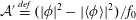 ${\mathcal{A}}^{\prime }\,\stackrel{def}{=}\,(|\unicode[STIX]{x1D719}|^{2}-|\langle \unicode[STIX]{x1D719}\rangle |^{2})/f_{0}$
; in figure 8(c) the early negative
${\mathcal{A}}^{\prime }\,\stackrel{def}{=}\,(|\unicode[STIX]{x1D719}|^{2}-|\langle \unicode[STIX]{x1D719}\rangle |^{2})/f_{0}$
; in figure 8(c) the early negative
 $r$
is nearly independent of dispersivity. Because significant energy exchange takes place in the anti-cyclones due to the initial wave concentration, a positive vorticity skewness ensues (figure 8
d). Once the eddy scales are created, advection strains the waves and generates further wave potential energy at the expense of balanced kinetic energy. It is in this stage that the dependence on dispersivity is pronounced: weakly dispersive waves are strained further than strongly dispersive waves. Thus the advective conversion becomes stronger with decreasing dispersivity (figure 8
b). Advection and dispersion significantly reduce the wave–vorticity correlation; the reduction in correlation increases as the dispersivity decreases (figure 8
c). For the weakest dispersivity considered, the wave–vorticity correlation becomes weakly positive, likely because of the early positive vorticity skewness.
$r$
is nearly independent of dispersivity. Because significant energy exchange takes place in the anti-cyclones due to the initial wave concentration, a positive vorticity skewness ensues (figure 8
d). Once the eddy scales are created, advection strains the waves and generates further wave potential energy at the expense of balanced kinetic energy. It is in this stage that the dependence on dispersivity is pronounced: weakly dispersive waves are strained further than strongly dispersive waves. Thus the advective conversion becomes stronger with decreasing dispersivity (figure 8
b). Advection and dispersion significantly reduce the wave–vorticity correlation; the reduction in correlation increases as the dispersivity decreases (figure 8
c). For the weakest dispersivity considered, the wave–vorticity correlation becomes weakly positive, likely because of the early positive vorticity skewness.
In all solutions reported above, the evolution of the balanced flow is similar to that of waveless 2-D turbulence: there is a transfer of balanced energy towards larger scales driven by merger of like-signed vortices; see figure 9(a). The main difference is that balanced kinetic energy is constantly transformed into wave potential energy via stimulated generation. The stimulated generation process is associated with a forward transfer of wave action
 ${\mathcal{A}}$
from the infinite horizontal scale in the initial condition (2.14) to the eddy scale; see figure 9(b). The wave potential energy density
${\mathcal{A}}$
from the infinite horizontal scale in the initial condition (2.14) to the eddy scale; see figure 9(b). The wave potential energy density
 ${\mathcal{P}}$
in figure 9(c) develops significantly smaller scales than those of the balanced kinetic energy
${\mathcal{P}}$
in figure 9(c) develops significantly smaller scales than those of the balanced kinetic energy
 ${\mathcal{K}}$
.
${\mathcal{K}}$
.
5 Wave escape
The expression for the energy conversion in (3.12) illuminates the physics of stimulated generation: both convergence of wave action density into anti-cyclones (3.14) and geostrophic straining of the wave field (3.16) are sources of wave potential energy and sinks of balanced kinetic energy. But this characterization of stimulated generation ignores the important role of wave dispersion – waves can propagate out of the vorticity or straining regions, thereby reducing the correlations
 $\unicode[STIX]{x1D6E4}_{r}$
and
$\unicode[STIX]{x1D6E4}_{r}$
and
 $\unicode[STIX]{x1D6E4}_{a}$
required for stimulated generation.
$\unicode[STIX]{x1D6E4}_{a}$
required for stimulated generation.
Wave dispersion is the only mechanism that upsets stimulated generation in the quasi-inviscid solutions described in this paper. In all solutions, after an initial conversion due to refraction, advective straining accounts for most of the energy conversion. Experience with the passive-scalar problem suggests (incorrectly) that the wave potential energy
 ${\mathcal{P}}$
should then increase exponentially with time as
${\mathcal{P}}$
should then increase exponentially with time as
 $\unicode[STIX]{x1D735}\unicode[STIX]{x1D719}$
is amplified by stirring (e.g. Young, Rhines & Garrett Reference Young, Rhines and Garrett1982). But even in the weakly dispersive limit, the waves do not behave as a passive scalar and stimulated generation is much less effective than suggested by this ‘passive-scalar thinking’. This is because advective straining can only increase
$\unicode[STIX]{x1D735}\unicode[STIX]{x1D719}$
is amplified by stirring (e.g. Young, Rhines & Garrett Reference Young, Rhines and Garrett1982). But even in the weakly dispersive limit, the waves do not behave as a passive scalar and stimulated generation is much less effective than suggested by this ‘passive-scalar thinking’. This is because advective straining can only increase
 $\unicode[STIX]{x1D735}\unicode[STIX]{x1D719}$
so much: the near-inertial generalized group velocity is
$\unicode[STIX]{x1D735}\unicode[STIX]{x1D719}$
so much: the near-inertial generalized group velocity is
 $\unicode[STIX]{x1D702}\unicode[STIX]{x1D735}\unicode[STIX]{x1D6E9}$
(cf. § 3), where
$\unicode[STIX]{x1D702}\unicode[STIX]{x1D735}\unicode[STIX]{x1D6E9}$
(cf. § 3), where
 $\unicode[STIX]{x1D6E9}$
is the phase of the near-inertial back-rotated velocity
$\unicode[STIX]{x1D6E9}$
is the phase of the near-inertial back-rotated velocity
 $\unicode[STIX]{x1D719}=|\unicode[STIX]{x1D719}|\text{e}^{\text{i}\unicode[STIX]{x1D6E9}}$
. Geostrophic straining enhances
$\unicode[STIX]{x1D719}=|\unicode[STIX]{x1D719}|\text{e}^{\text{i}\unicode[STIX]{x1D6E9}}$
. Geostrophic straining enhances
 $\unicode[STIX]{x1D735}\unicode[STIX]{x1D6E9}$
thereby increasing the near-inertial group velocity so that the waves escape the straining region. Thus, straining by a barotropic balanced flow results in near-inertial ‘wave escape’, as opposed to the ‘wave capture’ described by Bühler & McIntyre (Reference Bühler and McIntyre2005). Indeed, wave capture requires both lateral strain and vertical shear: the vertical-plane-wave model has no vertical shear and therefore wave capture is inoperative; see Thomas (Reference Thomas2012) for further discussion of the importance of vertical shear to wave capture.
$\unicode[STIX]{x1D735}\unicode[STIX]{x1D6E9}$
thereby increasing the near-inertial group velocity so that the waves escape the straining region. Thus, straining by a barotropic balanced flow results in near-inertial ‘wave escape’, as opposed to the ‘wave capture’ described by Bühler & McIntyre (Reference Bühler and McIntyre2005). Indeed, wave capture requires both lateral strain and vertical shear: the vertical-plane-wave model has no vertical shear and therefore wave capture is inoperative; see Thomas (Reference Thomas2012) for further discussion of the importance of vertical shear to wave capture.
5.1 Strain flow
We are surprised by the successful resistance mounted by the waves to strain-driven exponential amplification of
 $\unicode[STIX]{x1D735}\unicode[STIX]{x1D719}$
and thus seek to illustrate wave escape with simple flows. We first consider the straining flow
$\unicode[STIX]{x1D735}\unicode[STIX]{x1D719}$
and thus seek to illustrate wave escape with simple flows. We first consider the straining flow
 $\unicode[STIX]{x1D713}=-\unicode[STIX]{x1D6FC}xy$
. Ignoring dissipation for simplicity, the wave equation (2.8) reduces to
$\unicode[STIX]{x1D713}=-\unicode[STIX]{x1D6FC}xy$
. Ignoring dissipation for simplicity, the wave equation (2.8) reduces to
 $$\begin{eqnarray}\displaystyle & \displaystyle \unicode[STIX]{x1D719}_{t}+\unicode[STIX]{x1D6FC}x\unicode[STIX]{x1D719}_{x}-\unicode[STIX]{x1D6FC}y\unicode[STIX]{x1D719}_{y}-{\displaystyle \frac{\text{i}}{2}}\unicode[STIX]{x1D702}\unicode[STIX]{x0394}\unicode[STIX]{x1D719}=0, & \displaystyle\end{eqnarray}$$
and the action equation is
 $$\begin{eqnarray}\displaystyle & \displaystyle {\mathcal{A}}_{t}+\unicode[STIX]{x1D6FC}(x{\mathcal{A}})_{x}-\unicode[STIX]{x1D6FC}(y{\mathcal{A}})_{y}+\unicode[STIX]{x1D735}\boldsymbol{\cdot }\boldsymbol{{\mathcal{F}}}=0. & \displaystyle\end{eqnarray}$$
Without vorticity and dissipation, Ehrenfest’s theorem (3.11) reduces to
 $$\begin{eqnarray}\displaystyle & \displaystyle \unicode[STIX]{x2202}_{t}[\langle {\mathcal{F}}^{x}\rangle ,\,\langle {\mathcal{F}}^{y}\rangle ]=[-\unicode[STIX]{x1D6FC}\langle {\mathcal{F}}^{x}\rangle ,~+\unicode[STIX]{x1D6FC}\langle {\mathcal{F}}^{y}\rangle ], & \displaystyle\end{eqnarray}$$
with solution
 $$\begin{eqnarray}\displaystyle & \displaystyle [\langle {\mathcal{F}}^{x}\rangle ,\,\langle {\mathcal{F}}^{y}\rangle ]=[\langle {\mathcal{F}}^{x}\rangle _{0}\text{e}^{-\unicode[STIX]{x1D6FC}t},\,\langle {\mathcal{F}}^{y}\rangle _{0}\text{e}^{\unicode[STIX]{x1D6FC}t}], & \displaystyle\end{eqnarray}$$
where the subscript
 $0$
denotes the initial condition. For a compact wave packet, with a well-defined uniform group velocity
$0$
denotes the initial condition. For a compact wave packet, with a well-defined uniform group velocity
 $\boldsymbol{c}_{g}$
, the action flux is
$\boldsymbol{c}_{g}$
, the action flux is
 $$\begin{eqnarray}\displaystyle & \displaystyle \langle \boldsymbol{{\mathcal{F}}}\rangle =\boldsymbol{c}_{g}\langle {\mathcal{A}}\rangle . & \displaystyle\end{eqnarray}$$
Because
 $\langle {\mathcal{A}}\rangle$
is constant, (5.4) is thus also a solution for
$\langle {\mathcal{A}}\rangle$
is constant, (5.4) is thus also a solution for
 $\boldsymbol{c}_{g}(t)$
.
$\boldsymbol{c}_{g}(t)$
.
The position of the centre of the packet is
 $$\begin{eqnarray}\displaystyle & \displaystyle \boldsymbol{x}_{c}(t)\,\stackrel{def}{=}\,\langle \boldsymbol{x}{\mathcal{A}}\rangle /\langle {\mathcal{A}}\rangle . & \displaystyle\end{eqnarray}$$
Multiplying (5.2) by
 $\boldsymbol{x}$
, averaging and using (5.4), yields
$\boldsymbol{x}$
, averaging and using (5.4), yields
 $$\begin{eqnarray}\displaystyle & \displaystyle \unicode[STIX]{x2202}_{t}x_{c}-\unicode[STIX]{x1D6FC}x_{c}=c_{g0}^{x}\text{e}^{-\unicode[STIX]{x1D6FC}t},\quad \text{and}\quad \unicode[STIX]{x2202}_{t}y_{c}+\unicode[STIX]{x1D6FC}y_{c}=c_{g0}^{y}\text{e}^{\unicode[STIX]{x1D6FC}t}, & \displaystyle\end{eqnarray}$$
with solution
 $$\begin{eqnarray}\displaystyle & \displaystyle \boldsymbol{x}_{c}(t)=\boldsymbol{x}_{c0}+\boldsymbol{c}_{g0}{\displaystyle \frac{\sinh \unicode[STIX]{x1D6FC}t}{\unicode[STIX]{x1D6FC}}}. & \displaystyle\end{eqnarray}$$
The trajectory of the packet is therefore a straight line following the initial group velocity
 $\boldsymbol{c}_{g0}$
. The wave packet is not deflected by the hyperbolic streamlines of the straining flow and the packet escapes by accelerating exponentially with time along a straight-line trajectory. This requires that the group velocity
$\boldsymbol{c}_{g0}$
. The wave packet is not deflected by the hyperbolic streamlines of the straining flow and the packet escapes by accelerating exponentially with time along a straight-line trajectory. This requires that the group velocity
 $\boldsymbol{c}_{g}(t)$
adjusts in magnitude and direction so as to keep the centre of the packet on the straight and narrow.
$\boldsymbol{c}_{g}(t)$
adjusts in magnitude and direction so as to keep the centre of the packet on the straight and narrow.
The result in (5.8) is so remarkable that it is reassuring to obtain it without invoking Ehrenfest’s theorem. We thus consider the specific example of a wave packet launched in the strain field with the Gaussian initial condition
 $$\begin{eqnarray}\displaystyle & \displaystyle \unicode[STIX]{x1D719}(x,y,0)={\displaystyle \frac{2\unicode[STIX]{x03C0}}{\unicode[STIX]{x1D707}\unicode[STIX]{x1D708}}}\exp \left[-{\displaystyle \frac{1}{2}}\left({\displaystyle \frac{x^{2}}{\unicode[STIX]{x1D707}^{2}}}+{\displaystyle \frac{y^{2}}{\unicode[STIX]{x1D708}^{2}}}\right)+\text{i}(px+qy)\right]. & \displaystyle\end{eqnarray}$$
If
 $p\unicode[STIX]{x1D707}\gg 1$
and
$p\unicode[STIX]{x1D707}\gg 1$
and
 $q\unicode[STIX]{x1D708}\gg 1$
this is a wave packet with initial wavenumber
$q\unicode[STIX]{x1D708}\gg 1$
this is a wave packet with initial wavenumber
 $(p,q)$
and initial group velocity
$(p,q)$
and initial group velocity
 $$\begin{eqnarray}\displaystyle & \displaystyle \boldsymbol{c}_{g0}=\unicode[STIX]{x1D702}\,(p,q). & \displaystyle\end{eqnarray}$$
The exact solution to (5.1), subject to the initial condition (5.9), is
 $$\begin{eqnarray}\displaystyle \displaystyle \unicode[STIX]{x1D719} & = & \displaystyle {\displaystyle \frac{2\unicode[STIX]{x03C0}}{\sqrt{(\unicode[STIX]{x1D707}^{2}+\text{i}\unicode[STIX]{x1D702}f)(\unicode[STIX]{x1D708}^{2}+\text{i}\unicode[STIX]{x1D702}g)}}}\nonumber\\ \displaystyle & & \displaystyle \times \,\exp \left[-{\displaystyle \frac{1}{2}}{\displaystyle \frac{x^{2}\text{e}^{-2\unicode[STIX]{x1D6FC}t}-2\text{i}\unicode[STIX]{x1D707}^{2}px\text{e}^{-\unicode[STIX]{x1D6FC}t}+\text{i}\unicode[STIX]{x1D702}f\unicode[STIX]{x1D707}^{2}p^{2}}{\unicode[STIX]{x1D707}^{2}+\text{i}\unicode[STIX]{x1D702}f}}-{\displaystyle \frac{1}{2}}{\displaystyle \frac{y^{2}\text{e}^{2\unicode[STIX]{x1D6FC}t}-2\text{i}\unicode[STIX]{x1D708}^{2}qy\text{e}^{\unicode[STIX]{x1D6FC}t}+\text{i}\unicode[STIX]{x1D702}g\unicode[STIX]{x1D708}^{2}q^{2}}{\unicode[STIX]{x1D708}^{2}+\text{i}\unicode[STIX]{x1D702}g}}\right],\nonumber\\ \displaystyle & & \displaystyle\end{eqnarray}$$
with
 $$\begin{eqnarray}\displaystyle & \displaystyle f\,\stackrel{def}{=}\,{\displaystyle \frac{1-\text{e}^{-2\unicode[STIX]{x1D6FC}t}}{2\unicode[STIX]{x1D6FC}}}\quad \text{and}\quad g\,\stackrel{def}{=}\,{\displaystyle \frac{\text{e}^{2\unicode[STIX]{x1D6FC}t}-1}{2\unicode[STIX]{x1D6FC}}}. & \displaystyle\end{eqnarray}$$
Figure 10 illustrates the solution (5.11). The strain flow tilts the packet to align it with the
 $x$
-axis. The flow then exponentially stretches the packet, which in turn escapes from the saddle point. To calculate the trajectory of the packet we note that
$x$
-axis. The flow then exponentially stretches the packet, which in turn escapes from the saddle point. To calculate the trajectory of the packet we note that
 $$\begin{eqnarray}\displaystyle & \displaystyle |\unicode[STIX]{x1D719}|^{2}={\displaystyle \frac{(2\unicode[STIX]{x03C0})^{2}}{\sqrt{(\unicode[STIX]{x1D707}^{4}+\unicode[STIX]{x1D702}^{2}f^{2})(\unicode[STIX]{x1D708}^{4}+\unicode[STIX]{x1D702}^{2}g^{2})}}}\,\exp \left[-{\displaystyle \frac{\unicode[STIX]{x1D707}^{2}(x\text{e}^{-\unicode[STIX]{x1D6FC}t}-\unicode[STIX]{x1D702}fp)^{2}}{\unicode[STIX]{x1D707}^{4}+\unicode[STIX]{x1D702}^{2}f^{2}}}-{\displaystyle \frac{\unicode[STIX]{x1D708}^{2}(y\text{e}^{\unicode[STIX]{x1D6FC}t}-\unicode[STIX]{x1D702}gq)^{2}}{\unicode[STIX]{x1D708}^{4}+\unicode[STIX]{x1D702}^{2}g^{2}}}\right], & \displaystyle \nonumber\\ \displaystyle & & \displaystyle\end{eqnarray}$$
and we recover
 $\boldsymbol{x}_{c}(t)$
in (5.8) as the centre of the packet in (5.13).
$\boldsymbol{x}_{c}(t)$
in (5.8) as the centre of the packet in (5.13).

Figure 10. The escape of a Gaussian near-inertial wave packet from the saddle of a strain flow. The Gaussian decay scale is
 $\unicode[STIX]{x1D707}=\unicode[STIX]{x1D708}$
. The waves are weakly dispersive:
$\unicode[STIX]{x1D707}=\unicode[STIX]{x1D708}$
. The waves are weakly dispersive:
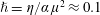 $\hslash =\unicode[STIX]{x1D702}/\unicode[STIX]{x1D6FC}\unicode[STIX]{x1D707}^{2}\approx 0.1$
. Black contours show the streamfunction
$\hslash =\unicode[STIX]{x1D702}/\unicode[STIX]{x1D6FC}\unicode[STIX]{x1D707}^{2}\approx 0.1$
. Black contours show the streamfunction
 $\unicode[STIX]{x1D713}=-\unicode[STIX]{x1D6FC}xy$
, and colours represent wave zonal velocity; the colour bar limits are fixed. The black dot indicates the centre of the packet and the grey line tracks its trail.
$\unicode[STIX]{x1D713}=-\unicode[STIX]{x1D6FC}xy$
, and colours represent wave zonal velocity; the colour bar limits are fixed. The black dot indicates the centre of the packet and the grey line tracks its trail.

Figure 11. A comparison of passive-scalar and wave solutions (
 $\hslash \approx 0.09$
) with same initial conditions (the wave kinetic energy is equal to the passive-scalar variance) and the same small-scale dissipation. (a) Initial condition of wave back-rotated zonal velocity and of the passive scalar. (b) Wave back-rotated zonal velocity at
$\hslash \approx 0.09$
) with same initial conditions (the wave kinetic energy is equal to the passive-scalar variance) and the same small-scale dissipation. (a) Initial condition of wave back-rotated zonal velocity and of the passive scalar. (b) Wave back-rotated zonal velocity at
 $t\times U_{e}k_{e}=10$
. (c) Passive-scalar concentration at
$t\times U_{e}k_{e}=10$
. (c) Passive-scalar concentration at
 $t\times U_{e}k_{e}=10$
. (d) Variance of wave velocity or passive-scalar variance. (e) Variance of wave velocity gradient or passive scalar. In (d) and (e), the diagnostics are normalized by their initial values.
$t\times U_{e}k_{e}=10$
. (d) Variance of wave velocity or passive-scalar variance. (e) Variance of wave velocity gradient or passive scalar. In (d) and (e), the diagnostics are normalized by their initial values.
5.2 A flow with strain and vorticity
As a second example of wave escape, figure 11 shows a numerical solution for a wave packet launched at the saddle point of a large-scale balanced flow with
 $\unicode[STIX]{x1D713}=\sin x+\sin y$
. The small-time evolution of the packet is predicted by the strain–flow solution discussed above. Figure 11(a–c) shows that the behaviour of the wave packet is qualitatively different from that of a passive scalar in the same flow: the passive scalar is stretched out along the separatrices while the wave packet escapes into the vortex centres. Thus the passive-scalar packet is strained and quickly diffused into oblivion. On the other hand, the waves are strained just so much, resulting in acceleration and escape from the straining region; the waves finally concentrate in the regions with non-zero vorticity, i.e. in the regions where the Okubo–Weiss criterion indicates no exponential stretching.
$\unicode[STIX]{x1D713}=\sin x+\sin y$
. The small-time evolution of the packet is predicted by the strain–flow solution discussed above. Figure 11(a–c) shows that the behaviour of the wave packet is qualitatively different from that of a passive scalar in the same flow: the passive scalar is stretched out along the separatrices while the wave packet escapes into the vortex centres. Thus the passive-scalar packet is strained and quickly diffused into oblivion. On the other hand, the waves are strained just so much, resulting in acceleration and escape from the straining region; the waves finally concentrate in the regions with non-zero vorticity, i.e. in the regions where the Okubo–Weiss criterion indicates no exponential stretching.
On the bottom row, figure 11(d) shows that while wave action
 $\propto |\unicode[STIX]{x1D719}|^{2}$
is nearly conserved, the analogous passive-scalar variance is strongly dissipated. Figure 11(e) shows that the variance of the passive-scalar gradient at first increases exponentially due to straining and then decays due to diffusion. On the other hand, the potential energy of the waves
$\propto |\unicode[STIX]{x1D719}|^{2}$
is nearly conserved, the analogous passive-scalar variance is strongly dissipated. Figure 11(e) shows that the variance of the passive-scalar gradient at first increases exponentially due to straining and then decays due to diffusion. On the other hand, the potential energy of the waves
 $\propto |\unicode[STIX]{x1D735}\unicode[STIX]{x1D719}|^{2}$
increases slowly and then oscillates around an equilibrium level. The wave-escape phenomenology in the turbulence solutions of § 4 qualitatively resembles that seen in this simple flow. In particular, the wave potential energy does not reach the dissipative scale (figure 9
c).
$\propto |\unicode[STIX]{x1D735}\unicode[STIX]{x1D719}|^{2}$
increases slowly and then oscillates around an equilibrium level. The wave-escape phenomenology in the turbulence solutions of § 4 qualitatively resembles that seen in this simple flow. In particular, the wave potential energy does not reach the dissipative scale (figure 9
c).
6 The Eulerian-mean viewpoint
In § 3 we developed conservation laws for
 ${\mathcal{A}}$
,
${\mathcal{A}}$
,
 ${\mathcal{P}}$
and
${\mathcal{P}}$
and
 ${\mathcal{K}}$
based on the Lagrangian-mean streamfunction
${\mathcal{K}}$
based on the Lagrangian-mean streamfunction
 $\unicode[STIX]{x1D713}$
and the back-rotated velocity
$\unicode[STIX]{x1D713}$
and the back-rotated velocity
 $\unicode[STIX]{x1D719}$
. Material conservation of PV is central to the NIW-QG system and thus the Lagrangian-mean velocity,
$\unicode[STIX]{x1D719}$
. Material conservation of PV is central to the NIW-QG system and thus the Lagrangian-mean velocity,
 $(-\unicode[STIX]{x1D713}_{y},\unicode[STIX]{x1D713}_{x})$
, must be a key field. But then
$(-\unicode[STIX]{x1D713}_{y},\unicode[STIX]{x1D713}_{x})$
, must be a key field. But then
 ${\mathcal{K}}=|\unicode[STIX]{x1D735}\unicode[STIX]{x1D713}|^{2}/2$
is not the kinetic energy of the Eulerian-mean velocity and therefore Reynolds stress diagnostics do not directly indicate changes in
${\mathcal{K}}=|\unicode[STIX]{x1D735}\unicode[STIX]{x1D713}|^{2}/2$
is not the kinetic energy of the Eulerian-mean velocity and therefore Reynolds stress diagnostics do not directly indicate changes in
 ${\mathcal{K}}$
. In fact Reynolds stresses have not been mentioned in § 3 and one might wonder how these standard statistics are related to the NIW-QG energy conversions
${\mathcal{K}}$
. In fact Reynolds stresses have not been mentioned in § 3 and one might wonder how these standard statistics are related to the NIW-QG energy conversions
 $\unicode[STIX]{x1D6E4}_{r}$
and
$\unicode[STIX]{x1D6E4}_{r}$
and
 $\unicode[STIX]{x1D6E4}_{a}$
. In this section we identify the Eulerian-mean energy transfers in terms of NIW-QG fields.
$\unicode[STIX]{x1D6E4}_{a}$
. In this section we identify the Eulerian-mean energy transfers in terms of NIW-QG fields.

Figure 12. Snapshot of the dipole Lagrangian-mean streamfunction and its decomposition into Eulerian-mean streamfunction and Stokes drift. The snapshot is at
 $t\times U_{e}k_{e}=10$
, just after the end of the refractive stage. The spatial average of each field was removed for direct comparison.
$t\times U_{e}k_{e}=10$
, just after the end of the refractive stage. The spatial average of each field was removed for direct comparison.
6.1 Kinetic energy of the Lagrangian-mean and Eulerian-mean flows
Appendix A.2 shows that in the vertical-plane-wave model, the Stokes drift is horizontally non-divergent, with streamfunction
 $-{\mathcal{A}}$
. Thus the Stokes velocity is
$-{\mathcal{A}}$
. Thus the Stokes velocity is
 $$\begin{eqnarray}\displaystyle & \displaystyle \boldsymbol{u}^{S}=-\hat{\boldsymbol{k}}\times \unicode[STIX]{x1D735}{\mathcal{A}}, & \displaystyle\end{eqnarray}$$
and the Eulerian-mean streamfunction is
 $$\begin{eqnarray}\displaystyle & \displaystyle \unicode[STIX]{x1D713}^{\text{E}}\,\stackrel{def}{=}\,\unicode[STIX]{x1D713}+{\mathcal{A}}. & \displaystyle\end{eqnarray}$$
To illustrate the important differences between Lagrangian-mean and Eulerian-mean viewpoints, figure 12 shows a snapshot of the dipole example from § 2.3. This snapshot was taken at
 $t\times U_{e}k_{e}=10$
, just after the end of the refractive stage of energy conversion, when waves are strongly concentrated in the anti-cyclone. While
$t\times U_{e}k_{e}=10$
, just after the end of the refractive stage of energy conversion, when waves are strongly concentrated in the anti-cyclone. While
 $\unicode[STIX]{x1D713}$
is fairly symmetric, the Eulerian-mean streamfunction
$\unicode[STIX]{x1D713}$
is fairly symmetric, the Eulerian-mean streamfunction
 $\unicode[STIX]{x1D713}^{\text{E}}$
displays a stronger anti-cyclone. The Stokes drift is concentrated in the negative
$\unicode[STIX]{x1D713}^{\text{E}}$
displays a stronger anti-cyclone. The Stokes drift is concentrated in the negative
 $\unicode[STIX]{x1D701}$
region and is anti-parallel to the Eulerian-mean flow. Thus the asymmetry in
$\unicode[STIX]{x1D701}$
region and is anti-parallel to the Eulerian-mean flow. Thus the asymmetry in
 $\unicode[STIX]{x1D713}^{\text{E}}$
is compensated by a strong ‘Stokes cyclone’, which is set up during the refractive stage and thus the Lagrangian-mean streamfunction
$\unicode[STIX]{x1D713}^{\text{E}}$
is compensated by a strong ‘Stokes cyclone’, which is set up during the refractive stage and thus the Lagrangian-mean streamfunction
 $\unicode[STIX]{x1D713}$
is more nearly a symmetric dipole.
$\unicode[STIX]{x1D713}$
is more nearly a symmetric dipole.
Using the decomposition (6.2), the balanced kinetic energy
 ${\mathcal{K}}=|\unicode[STIX]{x1D735}\unicode[STIX]{x1D713}|^{2}/2$
is
${\mathcal{K}}=|\unicode[STIX]{x1D735}\unicode[STIX]{x1D713}|^{2}/2$
is
 $$\begin{eqnarray}\displaystyle & \displaystyle {\mathcal{K}}=\underbrace{{\textstyle \frac{1}{2}}|\unicode[STIX]{x1D735}\unicode[STIX]{x1D713}^{\text{E}}|^{2}}_{\stackrel{def}{=}{\mathcal{K}}^{E}}+\underbrace{{\textstyle \frac{1}{2}}|\unicode[STIX]{x1D735}{\mathcal{A}}|^{2}-\unicode[STIX]{x1D735}\unicode[STIX]{x1D713}^{\text{E}}\boldsymbol{\cdot }\unicode[STIX]{x1D735}{\mathcal{A}}}_{\stackrel{def}{=}{\mathcal{K}}^{S}}. & \displaystyle\end{eqnarray}$$
 ${\mathcal{K}}$
does not diagonalize, i.e. the cross-term
${\mathcal{K}}$
does not diagonalize, i.e. the cross-term
 $\unicode[STIX]{x1D735}\unicode[STIX]{x1D713}^{\text{E}}\boldsymbol{\cdot }\unicode[STIX]{x1D735}{\mathcal{A}}$
is non-zero, and the ‘Stokes kinetic energy’
$\unicode[STIX]{x1D735}\unicode[STIX]{x1D713}^{\text{E}}\boldsymbol{\cdot }\unicode[STIX]{x1D735}{\mathcal{A}}$
is non-zero, and the ‘Stokes kinetic energy’
 ${\mathcal{K}}^{S}$
is not sign definite.
${\mathcal{K}}^{S}$
is not sign definite.
The first goal here is to obtain an expressions for the time rate of change of
 ${\mathcal{K}}^{S}$
and
${\mathcal{K}}^{S}$
and
 ${\mathcal{K}}^{E}$
. We begin with yet another
${\mathcal{K}}^{E}$
. We begin with yet another
 ${\mathcal{A}}$
-
${\mathcal{A}}$
-
 $\boldsymbol{{\mathcal{F}}}$
identity: using the definitions of
$\boldsymbol{{\mathcal{F}}}$
identity: using the definitions of
 ${\mathcal{A}}$
and
${\mathcal{A}}$
and
 $\boldsymbol{{\mathcal{F}}}$
in (3.1) and (3.6) yields
$\boldsymbol{{\mathcal{F}}}$
in (3.1) and (3.6) yields
 $$\begin{eqnarray}\displaystyle & \displaystyle {\mathcal{A}}\,\unicode[STIX]{x1D735}\boldsymbol{\cdot }(\hat{\boldsymbol{k}}\times \boldsymbol{{\mathcal{F}}})=-\boldsymbol{{\mathcal{F}}}\boldsymbol{\cdot }\hat{\boldsymbol{k}}\times \unicode[STIX]{x1D735}{\mathcal{A}}. & \displaystyle\end{eqnarray}$$
The average of (6.4), combined with a standard vector identities, results in
 $$\begin{eqnarray}\displaystyle & \displaystyle \langle {\mathcal{A}}\unicode[STIX]{x1D735}\boldsymbol{\cdot }(\hat{\boldsymbol{k}}\times \boldsymbol{{\mathcal{F}}})\rangle =\langle \boldsymbol{{\mathcal{F}}}\boldsymbol{\cdot }\hat{\boldsymbol{k}}\times \unicode[STIX]{x1D735}{\mathcal{A}}\rangle =0. & \displaystyle\end{eqnarray}$$
Equation (6.5) implies that the Stokes velocity
 $\boldsymbol{u}^{S}$
is, on average, orthogonal to the action flux
$\boldsymbol{u}^{S}$
is, on average, orthogonal to the action flux
 $\boldsymbol{{\mathcal{F}}}$
.
$\boldsymbol{{\mathcal{F}}}$
.
Forming
 $\langle {\mathcal{A}}q\rangle$
, and combining the expression for
$\langle {\mathcal{A}}q\rangle$
, and combining the expression for
 $q^{w}$
in (3.9) with the identity (6.5), yields
$q^{w}$
in (3.9) with the identity (6.5), yields
 $$\begin{eqnarray}\displaystyle & \displaystyle \langle {\mathcal{K}}^{S}\rangle =\langle {\mathcal{A}}q\rangle . & \displaystyle\end{eqnarray}$$
An expression for the rate of change of
 $\langle {\mathcal{K}}^{S}\rangle$
follows by combining the PV advection equation (2.7) with the action conservation (3.5):
$\langle {\mathcal{K}}^{S}\rangle$
follows by combining the PV advection equation (2.7) with the action conservation (3.5):
 $$\begin{eqnarray}\displaystyle & \displaystyle {\displaystyle \frac{\text{d}\langle {\mathcal{K}}^{S}\rangle }{\text{d}t}}=-\unicode[STIX]{x1D6E4}_{S}+\underbrace{\langle {\mathcal{A}}D_{q}\rangle +\langle qD_{{\mathcal{A}}}\rangle }_{\stackrel{def}{=}\unicode[STIX]{x1D700}_{S}}, & \displaystyle\end{eqnarray}$$
where
 $$\begin{eqnarray}\displaystyle & \displaystyle \unicode[STIX]{x1D6E4}_{S}\,\stackrel{def}{=}\,\langle q\unicode[STIX]{x1D735}\boldsymbol{\cdot }\boldsymbol{{\mathcal{F}}}\rangle . & \displaystyle\end{eqnarray}$$
Finally we obtain the rate of change of the Eulerian-mean kinetic energy by combining (6.7) with (3.13):
 $$\begin{eqnarray}\displaystyle & \displaystyle {\displaystyle \frac{\text{d}\langle {\mathcal{K}}^{E}\rangle }{\text{d}t}}=\unicode[STIX]{x1D6E4}_{S}-\unicode[STIX]{x1D6E4}_{r}-\unicode[STIX]{x1D6E4}_{a}+\unicode[STIX]{x1D6EF}+\unicode[STIX]{x1D700}_{{\mathcal{K}}}-\unicode[STIX]{x1D700}_{S}. & \displaystyle\end{eqnarray}$$
6.2 Reynolds stresses and buoyancy fluxes
Within the Eulerian framework the horizontal velocity is represented as
 $$\begin{eqnarray}\displaystyle & \displaystyle \boldsymbol{u}=\boldsymbol{u}^{E}+\tilde{\boldsymbol{u}}, & \displaystyle\end{eqnarray}$$
where superscript
 $E$
denotes the Eulerian-mean and tilde denotes the near-inertial wave velocity. With this decomposition, the Eulerian-mean velocity satisfies
$E$
denotes the Eulerian-mean and tilde denotes the near-inertial wave velocity. With this decomposition, the Eulerian-mean velocity satisfies
 $$\begin{eqnarray}\displaystyle & \displaystyle \boldsymbol{u}_{t}^{E}+\boldsymbol{u}^{E}\boldsymbol{\cdot }\unicode[STIX]{x1D735}\boldsymbol{u}^{E}+(\tilde{\boldsymbol{u}}\boldsymbol{\cdot }\unicode[STIX]{x1D735}\tilde{\boldsymbol{u}})^{E}+\hat{\boldsymbol{k}}\times f_{0}\boldsymbol{u}^{E}+\unicode[STIX]{x1D735}p^{E}=0. & \displaystyle\end{eqnarray}$$
(Dissipation is neglected in the following discussion.) As in the vertical plane-wave model, we confine attention to mean velocities independent of
 $z$
, so that
$z$
, so that
 $\boldsymbol{u}^{E}=(-\unicode[STIX]{x1D713}_{y}^{E},\unicode[STIX]{x1D713}_{x}^{E})$
where
$\boldsymbol{u}^{E}=(-\unicode[STIX]{x1D713}_{y}^{E},\unicode[STIX]{x1D713}_{x}^{E})$
where
 $\unicode[STIX]{x1D713}^{E}$
is the Eulerian-mean streamfunction introduced in (6.2). Forming
$\unicode[STIX]{x1D713}^{E}$
is the Eulerian-mean streamfunction introduced in (6.2). Forming
 $\langle \!\boldsymbol{u}^{E}\boldsymbol{\cdot }$
(6.11)
$\langle \!\boldsymbol{u}^{E}\boldsymbol{\cdot }$
(6.11)
 $\rangle$
yields
$\rangle$
yields
 $$\begin{eqnarray}\displaystyle & \displaystyle {\displaystyle \frac{\text{d}\langle {\mathcal{K}}^{E}\rangle }{\text{d}t}}=\underbrace{\langle (\tilde{v}^{2}-\tilde{u} ^{2})^{E}\,\unicode[STIX]{x1D713}_{xy}^{E}+(\tilde{u} \tilde{v})^{E}\,(\unicode[STIX]{x1D713}_{xx}^{E}-\unicode[STIX]{x1D713}_{yy}^{E})\rangle }_{\stackrel{def}{=}RSP}. & \displaystyle\end{eqnarray}$$
Above
 $RSP$
is the Reynolds shear production of Eulerian-mean kinetic energy. Comparing (6.12) with (6.9), and ignoring the dissipative contributions, we see that
$RSP$
is the Reynolds shear production of Eulerian-mean kinetic energy. Comparing (6.12) with (6.9), and ignoring the dissipative contributions, we see that
 $$\begin{eqnarray}\displaystyle & \displaystyle RSP=\unicode[STIX]{x1D6E4}_{S}-\unicode[STIX]{x1D6E4}_{r}-\unicode[STIX]{x1D6E4}_{a}. & \displaystyle\end{eqnarray}$$
We can also consider the source of near-inertial potential energy by starting with the wave buoyancy equation
 $$\begin{eqnarray}\displaystyle & \displaystyle \tilde{b}_{t}+\boldsymbol{u}^{E}\boldsymbol{\cdot }\unicode[STIX]{x1D735}\tilde{b}+\unicode[STIX]{x1D735}\boldsymbol{\cdot }[\tilde{\boldsymbol{u}}\tilde{b}-(\tilde{\boldsymbol{u}}\tilde{b})^{E}]+\tilde{w}N^{2}=0, & \displaystyle\end{eqnarray}$$
where we have confined attention to the vertical-plane-wave model so that
 $b^{E}=0$
. Multiplying (6.14) by
$b^{E}=0$
. Multiplying (6.14) by
 $\tilde{b}$
, taking the Eulerian average and then the domain average
$\tilde{b}$
, taking the Eulerian average and then the domain average
 $\langle \rangle$
, we have
$\langle \rangle$
, we have
 $$\begin{eqnarray}\displaystyle \displaystyle {\displaystyle \frac{\text{d}\langle {\mathcal{P}}\rangle }{\text{d}t}} & = & \displaystyle -\underbrace{\langle (\tilde{w}\tilde{b})^{E}\rangle }_{\stackrel{def}{=}BF},\end{eqnarray}$$
 $$\begin{eqnarray}\displaystyle & = & \displaystyle \unicode[STIX]{x1D6E4}_{r}+\unicode[STIX]{x1D6E4}_{a}.\end{eqnarray}$$
Above
 ${\mathcal{P}}=(\tilde{b}^{2})^{E}/2N^{2}$
is the wave potential energy and
${\mathcal{P}}=(\tilde{b}^{2})^{E}/2N^{2}$
is the wave potential energy and
 $BF$
is the buoyancy flux; we have used (3.12) to relate
$BF$
is the buoyancy flux; we have used (3.12) to relate
 $\unicode[STIX]{x1D6E4}_{r}$
and
$\unicode[STIX]{x1D6E4}_{r}$
and
 $\unicode[STIX]{x1D6E4}_{a}$
to the Eulerian-mean buoyancy flux.
$\unicode[STIX]{x1D6E4}_{a}$
to the Eulerian-mean buoyancy flux.
Finally, from balanced energy equation (3.13) and
 ${\mathcal{K}}={\mathcal{K}}^{E}+{\mathcal{K}}^{S}$
, we deduce that
${\mathcal{K}}={\mathcal{K}}^{E}+{\mathcal{K}}^{S}$
, we deduce that
 $$\begin{eqnarray}\displaystyle \displaystyle {\displaystyle \frac{\text{d}\langle {\mathcal{K}}^{S}\rangle }{\text{d}t}} & = & \displaystyle BF-RSP,\end{eqnarray}$$
 $$\begin{eqnarray}\displaystyle & = & \displaystyle -\unicode[STIX]{x1D6E4}_{S}.\end{eqnarray}$$
Figure 13(a) shows the decomposition of
 $\langle {\mathcal{K}}\rangle$
into
$\langle {\mathcal{K}}\rangle$
into
 $\langle {\mathcal{K}}^{E}\rangle$
and
$\langle {\mathcal{K}}^{E}\rangle$
and
 $\langle {\mathcal{K}}^{S}\rangle$
for the main 2-D turbulence solution discussed in § 4. In the initial condition there is no Stokes flow and
$\langle {\mathcal{K}}^{S}\rangle$
for the main 2-D turbulence solution discussed in § 4. In the initial condition there is no Stokes flow and
 ${\mathcal{K}}={\mathcal{K}}^{E}$
. Then in the refractive stage, the kinetic energy of the Eulerian-mean flow
${\mathcal{K}}={\mathcal{K}}^{E}$
. Then in the refractive stage, the kinetic energy of the Eulerian-mean flow
 $\langle {\mathcal{K}}^{E}\rangle$
increases, while kinetic energy of the Lagrangian-mean flow
$\langle {\mathcal{K}}^{E}\rangle$
increases, while kinetic energy of the Lagrangian-mean flow
 $\langle {\mathcal{K}}\rangle$
decreases; the ‘Stokes energy’,
$\langle {\mathcal{K}}\rangle$
decreases; the ‘Stokes energy’,
 ${\mathcal{K}}^{S}={\mathcal{K}}-{\mathcal{K}}^{E}$
, is initially zero and becomes negative, due to a positive
${\mathcal{K}}^{S}={\mathcal{K}}-{\mathcal{K}}^{E}$
, is initially zero and becomes negative, due to a positive
 $\unicode[STIX]{x1D713}^{\text{E}}$
-
$\unicode[STIX]{x1D713}^{\text{E}}$
-
 ${\mathcal{A}}$
correlation (cf. figure 12). As illustrated in figure 12, the refractive stage, which creates the strong spatial modulations in action density
${\mathcal{A}}$
correlation (cf. figure 12). As illustrated in figure 12, the refractive stage, which creates the strong spatial modulations in action density
 ${\mathcal{A}}$
, can also be viewed as setting up the Stokes velocity in (6.1).
${\mathcal{A}}$
, can also be viewed as setting up the Stokes velocity in (6.1).

Figure 13. Diagnostics of the 2-D turbulence solution with parameters presented in table 4. (a) Kinetic energy change about initial condition. (b) Refractive and advective conversion terms, and shear production.
In the refractive stage, the advective conversion
 $\unicode[STIX]{x1D6E4}_{a}$
is small and
$\unicode[STIX]{x1D6E4}_{a}$
is small and
 $\unicode[STIX]{x1D6E4}_{S}\approx 2\unicode[STIX]{x1D6E4}_{r}$
. Hence the shear production is due to the refractive conversion,
$\unicode[STIX]{x1D6E4}_{S}\approx 2\unicode[STIX]{x1D6E4}_{r}$
. Hence the shear production is due to the refractive conversion,
 $RSP\approx \unicode[STIX]{x1D6E4}_{r}$
(see figure 13
b). At later times, during the advective stage,
$RSP\approx \unicode[STIX]{x1D6E4}_{r}$
(see figure 13
b). At later times, during the advective stage,
 $\unicode[STIX]{x1D6E4}_{S}-\unicode[STIX]{x1D6E4}_{r}$
is small, and therefore
$\unicode[STIX]{x1D6E4}_{S}-\unicode[STIX]{x1D6E4}_{r}$
is small, and therefore
 $RSP\approx BF\approx -\unicode[STIX]{x1D6E4}_{a}$
. At this stage,
$RSP\approx BF\approx -\unicode[STIX]{x1D6E4}_{a}$
. At this stage,
 $\unicode[STIX]{x2202}_{t}\langle {\mathcal{K}}\rangle \approx \unicode[STIX]{x2202}_{t}\langle K^{E}\rangle$
, and the connection between the Eulerian-mean and Lagrangian-mean viewpoints is straightforward: the kinetic energy extracted from the Eulerian-mean flow via Reynolds shear production approximately matches the creation of wave potential energy through buoyancy fluxes. In general, however, the connection is convoluted, involving the rate of change of the ‘Stokes energy’ in (6.17).
$\unicode[STIX]{x2202}_{t}\langle {\mathcal{K}}\rangle \approx \unicode[STIX]{x2202}_{t}\langle K^{E}\rangle$
, and the connection between the Eulerian-mean and Lagrangian-mean viewpoints is straightforward: the kinetic energy extracted from the Eulerian-mean flow via Reynolds shear production approximately matches the creation of wave potential energy through buoyancy fluxes. In general, however, the connection is convoluted, involving the rate of change of the ‘Stokes energy’ in (6.17).
7 Discussion and conclusions
7.1 Absence of a direct cascade of wave energy
The solutions reported here introduce the waves at
 $t=0$
in (2.14) with infinite spatial scale. Wave refraction,
$t=0$
in (2.14) with infinite spatial scale. Wave refraction,
 $\text{i}\unicode[STIX]{x1D719}\unicode[STIX]{x1D701}/2$
in (2.8), immediately transfers wave energy to the smaller scales of the balanced relative vorticity
$\text{i}\unicode[STIX]{x1D719}\unicode[STIX]{x1D701}/2$
in (2.8), immediately transfers wave energy to the smaller scales of the balanced relative vorticity
 $\unicode[STIX]{x1D701}$
. This giant leap across wavenumbers is not a direct cascade of wave energy in the sense of Kolmogorov. And because of wave escape, the wave energy that is so efficiently transferred to eddy scales by refraction does not undergo a turbulence-driven direct cascade to the small length scales at which the wave dissipation in (2.9) is effective. This conclusion hinges on the assumption of a barotropic balanced flow and fixed vertical wavenumber. Similar to the vertical-plane-wave model, shallow-water models lack wave capture and an efficient direct cascade of wave energy (e.g. McIntyre Reference McIntyre2009). In less idealized models with balanced baroclinic shear, the vertical wavenumber can increase, and a direct cascade, perhaps resulting in wave capture, can ensue; stimulated generation might then be much stronger than in the vertical-plane-wave model considered here.
$\unicode[STIX]{x1D701}$
. This giant leap across wavenumbers is not a direct cascade of wave energy in the sense of Kolmogorov. And because of wave escape, the wave energy that is so efficiently transferred to eddy scales by refraction does not undergo a turbulence-driven direct cascade to the small length scales at which the wave dissipation in (2.9) is effective. This conclusion hinges on the assumption of a barotropic balanced flow and fixed vertical wavenumber. Similar to the vertical-plane-wave model, shallow-water models lack wave capture and an efficient direct cascade of wave energy (e.g. McIntyre Reference McIntyre2009). In less idealized models with balanced baroclinic shear, the vertical wavenumber can increase, and a direct cascade, perhaps resulting in wave capture, can ensue; stimulated generation might then be much stronger than in the vertical-plane-wave model considered here.
7.2 Regimes of wave-modified turbulence
Geostrophic straining accounts for most of the stimulated generation of wave energy in the examples considered in this paper. But refraction plays a fundamental role in these solutions with the uniform initial wave velocity in (2.14), because refraction creates the initial gradients of wave velocity that are then enhanced by geostrophic straining. We experimented by changing the initial condition of
 $\unicode[STIX]{x1D719}$
to an eddy-scale plane wave and repeated all the 2-D turbulence solutions; the different initial condition significantly suppresses the initial refraction stage, but otherwise yields long-term solutions that are qualitatively similar to the solutions discussed above. Thus, to the extent that the uniform-wave initial condition (2.14) idealizes the generation of large-scale upper-ocean inertial oscillations by storms (e.g. Moehlis & Llewellyn Smith Reference Moehlis and Llewellyn Smith2001; Danioux et al.
Reference Danioux, Vanneste and Bühler2015), the initial refraction is a loss of lateral coherence, or a type of inertial pumping (Young & Ben Jelloul Reference Young and Ben Jelloul1997; Klein, Llewellyn Smith & Lapeyre Reference Klein, Llewellyn Smith and Lapeyre2004), which is accompanied by an extraction of energy from the balanced flow by the waves.
$\unicode[STIX]{x1D719}$
to an eddy-scale plane wave and repeated all the 2-D turbulence solutions; the different initial condition significantly suppresses the initial refraction stage, but otherwise yields long-term solutions that are qualitatively similar to the solutions discussed above. Thus, to the extent that the uniform-wave initial condition (2.14) idealizes the generation of large-scale upper-ocean inertial oscillations by storms (e.g. Moehlis & Llewellyn Smith Reference Moehlis and Llewellyn Smith2001; Danioux et al.
Reference Danioux, Vanneste and Bühler2015), the initial refraction is a loss of lateral coherence, or a type of inertial pumping (Young & Ben Jelloul Reference Young and Ben Jelloul1997; Klein, Llewellyn Smith & Lapeyre Reference Klein, Llewellyn Smith and Lapeyre2004), which is accompanied by an extraction of energy from the balanced flow by the waves.
Although 10–20 % of the balanced kinetic energy is converted into wave potential energy, and despite the wave breakage of the symmetry between cyclones and anti-cyclones, the wave-modified turbulence in § 4 remarkably resembles waveless two-dimensional turbulence (e.g. McWilliams Reference McWilliams1984): we still observe robust vortices and an increase in vortex length scale due to merger of like-signed vortices. Figure 7 shows small changes in the potential vorticity
 $q$
and much larger changes in the wave PV
$q$
and much larger changes in the wave PV
 $q^{w}$
induced by changing the dispersivity. In this sense, the turbulent evolution is insensitive to wave modification.
$q^{w}$
induced by changing the dispersivity. In this sense, the turbulent evolution is insensitive to wave modification.
To see significant wave modification of the turbulence we increased the amplitude of the initial wave in (2.14) so that
 $U_{w}=6U_{e}$
(in § 4,
$U_{w}=6U_{e}$
(in § 4,
 $U_{w}=2U_{e}$
). With this level of wave energy the wave-modified 2-D turbulence differs qualitatively from the waveless variety (not shown). The potential vorticity develops highly filamentary structures with little vortex formation; this inhibition of vortex formation is stronger in the weakly dispersive limit.
$U_{w}=2U_{e}$
). With this level of wave energy the wave-modified 2-D turbulence differs qualitatively from the waveless variety (not shown). The potential vorticity develops highly filamentary structures with little vortex formation; this inhibition of vortex formation is stronger in the weakly dispersive limit.
7.3 Energy transfers can be bi-directional in non-turbulent balanced flows
In all solutions considered in §§ 2 and 4, the energy transfer is always from the balanced flow into the waves. This positive energy conversion,
 $\unicode[STIX]{x1D6E4}_{r}+\unicode[STIX]{x1D6E4}_{a}>0$
, remains true for very long turbulence simulations (not shown), because the refractive conversion is small at large time and turbulent stirring always increases lateral wave gradients:
$\unicode[STIX]{x1D6E4}_{r}+\unicode[STIX]{x1D6E4}_{a}>0$
, remains true for very long turbulence simulations (not shown), because the refractive conversion is small at large time and turbulent stirring always increases lateral wave gradients:
 $\unicode[STIX]{x1D6E4}_{r}+\unicode[STIX]{x1D6E4}_{a}\approx \unicode[STIX]{x1D6E4}_{a}>0$
.
$\unicode[STIX]{x1D6E4}_{r}+\unicode[STIX]{x1D6E4}_{a}\approx \unicode[STIX]{x1D6E4}_{a}>0$
.
But the energy transfers can be bi-directional for non-turbulent flows. To illustrate this process, we consider a solution with initially uniform wave and
 $\unicode[STIX]{x1D713}(\boldsymbol{x},0)=\sin x+\sin y$
. This non-turbulent balanced flow consists of two vortices of opposite signs; there can be no inverse cascade from this initial condition because
$\unicode[STIX]{x1D713}(\boldsymbol{x},0)=\sin x+\sin y$
. This non-turbulent balanced flow consists of two vortices of opposite signs; there can be no inverse cascade from this initial condition because
 $\unicode[STIX]{x1D713}(\boldsymbol{x},0)$
is already at the domain scale. Starting from the initial uniform wave, the refractive conversion generates wave potential energy
$\unicode[STIX]{x1D713}(\boldsymbol{x},0)$
is already at the domain scale. Starting from the initial uniform wave, the refractive conversion generates wave potential energy
 ${\mathcal{P}}$
at the expense of balanced kinetic energy
${\mathcal{P}}$
at the expense of balanced kinetic energy
 ${\mathcal{K}}$
(figure 14). After this initial refractive stage, however,
${\mathcal{K}}$
(figure 14). After this initial refractive stage, however,
 ${\mathcal{P}}$
and
${\mathcal{P}}$
and
 ${\mathcal{K}}$
oscillate about equilibrium levels and there are quasi-periodic energy transfers back and forth between
${\mathcal{K}}$
oscillate about equilibrium levels and there are quasi-periodic energy transfers back and forth between
 ${\mathcal{P}}$
and
${\mathcal{P}}$
and
 ${\mathcal{K}}$
. In this solution, the refractive conversion
${\mathcal{K}}$
. In this solution, the refractive conversion
 $\unicode[STIX]{x1D6E4}_{r}$
accounts for most of the quasi-periodic exchanges between
$\unicode[STIX]{x1D6E4}_{r}$
accounts for most of the quasi-periodic exchanges between
 ${\mathcal{K}}$
and
${\mathcal{K}}$
and
 ${\mathcal{P}}$
.
${\mathcal{P}}$
.

Figure 14. Diagnostics of an illustrative solution with initially uniform wave and
 $\unicode[STIX]{x1D713}(t=0)=\sin x+\sin y$
, with
$\unicode[STIX]{x1D713}(t=0)=\sin x+\sin y$
, with
 $\unicode[STIX]{x1D6FC}=0.1$
and
$\unicode[STIX]{x1D6FC}=0.1$
and
 $\hslash =2$
. (a) Energy difference about initial condition. (b) Wave potential energy budget.
$\hslash =2$
. (a) Energy difference about initial condition. (b) Wave potential energy budget.
7.4 The correlation of wave amplitude with relative vorticity
A secondary result is the strong time dependence of the correlation
 $r$
, defined in (4.7), between incoherent waves and the relative vorticity;
$r$
, defined in (4.7), between incoherent waves and the relative vorticity;
 $r$
measures the concentration of waves into cyclones or anti-cyclones (Danioux et al.
Reference Danioux, Vanneste and Bühler2015). Refraction concentrates waves into anti-cyclones and expels them from cyclones, thereby generating an initial strong negative
$r$
measures the concentration of waves into cyclones or anti-cyclones (Danioux et al.
Reference Danioux, Vanneste and Bühler2015). Refraction concentrates waves into anti-cyclones and expels them from cyclones, thereby generating an initial strong negative
 $r$
(see figure 8
c). And Ehrenfest’s theorem provides perhaps the simplest explanation for this concentration – see (3.17). As conjectured by Danioux et al. (Reference Danioux, Vanneste and Bühler2015), the subsequent return of
$r$
(see figure 8
c). And Ehrenfest’s theorem provides perhaps the simplest explanation for this concentration – see (3.17). As conjectured by Danioux et al. (Reference Danioux, Vanneste and Bühler2015), the subsequent return of
 $r$
towards zero (and even to positive values in the case
$r$
towards zero (and even to positive values in the case
 $\hslash =0.5$
) is partially due to the unsteady geostrophic advection. The NIW-QG coupling compounds the unsteady advection: the dramatic initial concentration of waves into anti-cyclones weakens those vortices, with ensuing development of positive skewness of relative vorticity (see figure 8
d); the vorticity skewness increases with decreasing dispersivity because weakly dispersive waves extract more energy from the balanced flow (see figure 8).
$\hslash =0.5$
) is partially due to the unsteady geostrophic advection. The NIW-QG coupling compounds the unsteady advection: the dramatic initial concentration of waves into anti-cyclones weakens those vortices, with ensuing development of positive skewness of relative vorticity (see figure 8
d); the vorticity skewness increases with decreasing dispersivity because weakly dispersive waves extract more energy from the balanced flow (see figure 8).
7.5 Reconciling action conservation with
$RSP$
of wave kinetic energy

A main difficulty in making a connection between the NIW-QG model and earlier studies, such as those in table 1, is that the theory uses the Lagrangian-mean geostrophic flow as a primary variable. Previous studies generally employ an Eulerian wave-mean decomposition. Taylor & Straub (Reference Taylor and Straub2016), for example, use frequency filtering to separate low-frequency motions (Eulerian mean) from high-frequency flow (dominated by near-inertial waves). Taylor & Straub find energy exchange between low-frequency (eddy) kinetic energy and high-frequency (near-inertial) kinetic energy resulting from both vertical and horizontal Reynolds stresses; Taylor & Straub refer to this energy transfer as the ‘advective sink’, meaning a sink of low-frequency, Eulerian-mean kinetic energy. The Reynolds shear production
 $RSP$
in (6.12) is analogous to the horizontal part of the advective sink.
$RSP$
in (6.12) is analogous to the horizontal part of the advective sink.
The Reynolds stresses diagnostics of prior studies in table 1 might seem incompatible with fundamental aspects of the NIW-QG system. For example, the wave action
 ${\mathcal{A}}$
in (3.1) differs from the wave kinetic energy
${\mathcal{A}}$
in (3.1) differs from the wave kinetic energy
 $|\unicode[STIX]{x1D719}|^{2}/2$
only by the constant factor
$|\unicode[STIX]{x1D719}|^{2}/2$
only by the constant factor
 $f_{0}$
. Thus NIW-QG action conservation seems inconsistent with Reynolds stress transfer of kinetic energy from eddies to waves. But this impression is incorrect: Reynolds stresses are not inconsistent with conservation of
$f_{0}$
. Thus NIW-QG action conservation seems inconsistent with Reynolds stress transfer of kinetic energy from eddies to waves. But this impression is incorrect: Reynolds stresses are not inconsistent with conservation of
 ${\mathcal{A}}$
, nor with stimulated generation.
${\mathcal{A}}$
, nor with stimulated generation.
To understand this, note that conservation of
 ${\mathcal{A}}$
in (3.10) is a statement about the leading-order wave velocities encoded in
${\mathcal{A}}$
in (3.10) is a statement about the leading-order wave velocities encoded in
 $\unicode[STIX]{x1D719}$
; the balanced kinetic energy
$\unicode[STIX]{x1D719}$
; the balanced kinetic energy
 ${\mathcal{K}}$
also involves higher-order wave kinetic energy in the form of the ‘Stokes kinetic energy’
${\mathcal{K}}$
also involves higher-order wave kinetic energy in the form of the ‘Stokes kinetic energy’
 ${\mathcal{K}}^{S}$
: see (6.3) and the surrounding discussion. A main point from § 6.2 is that the energy transferred from the Eulerian-mean velocity by
${\mathcal{K}}^{S}$
: see (6.3) and the surrounding discussion. A main point from § 6.2 is that the energy transferred from the Eulerian-mean velocity by
 $RSP$
is accounted for by
$RSP$
is accounted for by
 ${\mathcal{K}}^{S}$
(rather than the leading-order wave kinetic energy
${\mathcal{K}}^{S}$
(rather than the leading-order wave kinetic energy
 $f_{0}{\mathcal{A}}$
).
$f_{0}{\mathcal{A}}$
).
At first glance it might seem that because stimulated generation results in an increase in wave potential energy
 ${\mathcal{P}}$
, it must necessarily involve a transfer from eddy potential energy. The vertical-plane-wave model is a counterexample: the eddies are barotropic and there is therefore no eddy potential energy to transfer. Indeed, if the eddies are barotropic, then
${\mathcal{P}}$
, it must necessarily involve a transfer from eddy potential energy. The vertical-plane-wave model is a counterexample: the eddies are barotropic and there is therefore no eddy potential energy to transfer. Indeed, if the eddies are barotropic, then
 $RSP$
is the only pathway between the Eulerian-mean kinetic energy
$RSP$
is the only pathway between the Eulerian-mean kinetic energy
 ${\mathcal{K}}^{E}$
and wave energy. This rather obvious fact is deeply hidden by the Lagrangian-mean average: the
${\mathcal{K}}^{E}$
and wave energy. This rather obvious fact is deeply hidden by the Lagrangian-mean average: the
 $RSP$
transfer out of
$RSP$
transfer out of
 ${\mathcal{K}}^{E}$
passes first through
${\mathcal{K}}^{E}$
passes first through
 ${\mathcal{K}}^{S}$
on the way to
${\mathcal{K}}^{S}$
on the way to
 ${\mathcal{P}}$
. The intermediate passage through
${\mathcal{P}}$
. The intermediate passage through
 ${\mathcal{K}}^{S}$
is an inevitable aspect of the Lagrangian-mean formulation of the NIW-QG system. All of these transfers can be diagnosed using
${\mathcal{K}}^{S}$
is an inevitable aspect of the Lagrangian-mean formulation of the NIW-QG system. All of these transfers can be diagnosed using
 $\unicode[STIX]{x1D6E4}_{a}$
,
$\unicode[STIX]{x1D6E4}_{a}$
,
 $\unicode[STIX]{x1D6E4}_{r}$
and
$\unicode[STIX]{x1D6E4}_{r}$
and
 $\unicode[STIX]{x1D6E4}_{S}$
and (6.13) relates Reynolds shear production to the three
$\unicode[STIX]{x1D6E4}_{S}$
and (6.13) relates Reynolds shear production to the three
 $\unicode[STIX]{x1D6E4}$
values.
$\unicode[STIX]{x1D6E4}$
values.
A full investigation of NIW-QG energetics, including diagnosis of
 $\unicode[STIX]{x1D6E4}_{r}$
,
$\unicode[STIX]{x1D6E4}_{r}$
,
 $\unicode[STIX]{x1D6E4}_{a}$
and
$\unicode[STIX]{x1D6E4}_{a}$
and
 $\unicode[STIX]{x1D6E4}_{S}$
in solutions of the Boussinesq equations, is beyond the scope of this article. But we emphasize a crucial simplifying feature of the NIW-QG approximation: there are no important Stokes corrections to pressure and buoyancy, and therefore, to leading order, the Lagrangian-mean velocity is equal to the balanced velocity based on an Eulerian-mean pressure field. In principle, this is a straightforward way of diagnosing Lagrangian-mean velocities from numerical solutions of the Boussinesq equations.
$\unicode[STIX]{x1D6E4}_{S}$
in solutions of the Boussinesq equations, is beyond the scope of this article. But we emphasize a crucial simplifying feature of the NIW-QG approximation: there are no important Stokes corrections to pressure and buoyancy, and therefore, to leading order, the Lagrangian-mean velocity is equal to the balanced velocity based on an Eulerian-mean pressure field. In principle, this is a straightforward way of diagnosing Lagrangian-mean velocities from numerical solutions of the Boussinesq equations.
7.6 Final remarks
There are many caveats to the application of our results to the post-storm oceanographic problem. Notably, the lack of geostrophic vertical shear suppresses important mechanisms of vertical refraction and straining, which introduce interesting modifications of the near-inertial wave physics (e.g. Thomas Reference Thomas2012) and can produce strong energy extraction by near-inertial waves (Shakespeare & Hogg Reference Shakespeare and Hogg2017). And our focus on quasi-inviscid initial value problems downplays the role of dissipation, but in forced-dissipative solutions, wave dissipation likely controls the strength of stimulated generation. Finally, better understanding the connection between numerical modelling studies (e.g. Taylor & Straub Reference Taylor and Straub2016) and the NIW-QG theory (XV; Wagner & Young Reference Wagner and Young2016) deserves further investigation. We hope to explore these topics in future work.
Acknowledgements
We thank three anonymous referees for constructive criticism and suggestions. This study was supported by the National Aeronautics and Space Administration (NNX16AO5OH) and the National Science Foundation (OCE-1357047 and OCE-1657041).
Appendix A. Details of the NIW-QG model
A.1 The NIW-QG model
Using multiscale asymptotic theory, Wagner & Young (Reference Wagner and Young2016) derive a model for the coupled evolution of QG balanced flow, near-inertial waves and their second harmonic. Assuming that the second harmonic is zero (
 $B=0$
), the Wagner & Young (Reference Wagner and Young2016) coupled model recovers the XV model in the limit where the waves have vertical scales much smaller than the balanced flow. In Wagner & Young (Reference Wagner and Young2016), the PV is
$B=0$
), the Wagner & Young (Reference Wagner and Young2016) coupled model recovers the XV model in the limit where the waves have vertical scales much smaller than the balanced flow. In Wagner & Young (Reference Wagner and Young2016), the PV is
 $$\begin{eqnarray}\displaystyle & \displaystyle q=(\unicode[STIX]{x0394}+L)\unicode[STIX]{x1D713}+\unicode[STIX]{x1D6FD}y+{\displaystyle \frac{1}{2f_{0}}}\left[\unicode[STIX]{x0394}{\displaystyle \frac{1}{2}}|LA|^{2}+\text{i}J(LA^{\star },LA)\right], & \displaystyle\end{eqnarray}$$
where
 $\unicode[STIX]{x0394}\,\stackrel{def}{=}\,\unicode[STIX]{x2202}_{x}^{2}+\unicode[STIX]{x2202}_{y}^{2}$
and
$\unicode[STIX]{x0394}\,\stackrel{def}{=}\,\unicode[STIX]{x2202}_{x}^{2}+\unicode[STIX]{x2202}_{y}^{2}$
and
 $L\,\stackrel{def}{=}\,\unicode[STIX]{x2202}_{z}(f_{0}/N)^{2}\unicode[STIX]{x2202}_{z}$
, and
$L\,\stackrel{def}{=}\,\unicode[STIX]{x2202}_{z}(f_{0}/N)^{2}\unicode[STIX]{x2202}_{z}$
, and
 $LA$
is the back-rotated near-inertial velocity; the leading-order wave plus balanced flow velocity is
$LA$
is the back-rotated near-inertial velocity; the leading-order wave plus balanced flow velocity is
 $$\begin{eqnarray}\displaystyle & \displaystyle u+\text{i}v=LA\text{e}^{-\text{i}f_{0}t}-\unicode[STIX]{x1D713}_{y}+\text{i}\unicode[STIX]{x1D713}_{x}, & \displaystyle\end{eqnarray}$$
where
 $\unicode[STIX]{x1D713}$
is the streamfunction of the Lagrangian-mean (geostrophically balanced) flow. The PV is materially conserved,
$\unicode[STIX]{x1D713}$
is the streamfunction of the Lagrangian-mean (geostrophically balanced) flow. The PV is materially conserved,
 $$\begin{eqnarray}\displaystyle & \displaystyle q_{t}+J(\unicode[STIX]{x1D713},q)=0, & \displaystyle\end{eqnarray}$$
and the wave back-rotated velocity satisfies the YBJ equation,
 $$\begin{eqnarray}\displaystyle & \displaystyle LA_{t}+{\displaystyle \frac{\text{i}}{2}}f_{0}\unicode[STIX]{x0394}A+J(\unicode[STIX]{x1D713},LA)+\text{i}LA\left({\displaystyle \frac{1}{2}}\unicode[STIX]{x0394}\unicode[STIX]{x1D713}+\unicode[STIX]{x1D6FD}y\right)=0. & \displaystyle\end{eqnarray}$$
The special family of solutions with a barotropic balanced flow
 $\unicode[STIX]{x1D713}=\unicode[STIX]{x1D713}(x,y,t)$
,
$\unicode[STIX]{x1D713}=\unicode[STIX]{x1D713}(x,y,t)$
,
 $f$
-plane (
$f$
-plane (
 $\unicode[STIX]{x1D6FD}=0$
), uniform background buoyancy frequency
$\unicode[STIX]{x1D6FD}=0$
), uniform background buoyancy frequency
 $N=N_{0}$
and
$N=N_{0}$
and
 $LA=\text{e}^{\text{i}mz}\,\unicode[STIX]{x1D719}(x,y)$
wave velocity yields the vertical-plane-wave model in (2.7)–(2.8). The plane-wave model is a solution of both XV and Wagner & Young (Reference Wagner and Young2016) equations because the barotropic flow assumption yields an infinite vertical scale separation between waves and balanced flow.
$LA=\text{e}^{\text{i}mz}\,\unicode[STIX]{x1D719}(x,y)$
wave velocity yields the vertical-plane-wave model in (2.7)–(2.8). The plane-wave model is a solution of both XV and Wagner & Young (Reference Wagner and Young2016) equations because the barotropic flow assumption yields an infinite vertical scale separation between waves and balanced flow.
A.2 Stokes drift
The horizontal component the Stokes drift of near-inertial waves is (Wagner & Young Reference Wagner and Young2016)
 $$\begin{eqnarray}\displaystyle & \displaystyle u^{S}+\text{i}v^{S}={\displaystyle \frac{\text{i}}{f_{0}}}(M_{zz}\unicode[STIX]{x2202}^{\star }M^{\star }-M_{z}^{\star }\unicode[STIX]{x2202}^{\star }M_{z}), & \displaystyle\end{eqnarray}$$
 $$\begin{eqnarray}\displaystyle & \displaystyle w^{S}={\displaystyle \frac{\text{i}}{f_{0}}}(M_{z}^{\star }\unicode[STIX]{x2202}\unicode[STIX]{x2202}^{\star }M-\unicode[STIX]{x2202}M_{z}\unicode[STIX]{x2202}^{\star }M)+\text{c.c.}, & \displaystyle\end{eqnarray}$$
where
 $M=(f_{0}/N)^{2}A_{z}$
and
$M=(f_{0}/N)^{2}A_{z}$
and
 $M_{z}=LA$
, and we recall
$M_{z}=LA$
, and we recall
 $\unicode[STIX]{x2202}=(\unicode[STIX]{x2202}_{x}-\text{i}\unicode[STIX]{x2202}_{y})/2$
. In the vertical-plane-wave model, the back-rotated velocity is
$\unicode[STIX]{x2202}=(\unicode[STIX]{x2202}_{x}-\text{i}\unicode[STIX]{x2202}_{y})/2$
. In the vertical-plane-wave model, the back-rotated velocity is
 $M_{z}=\unicode[STIX]{x1D719}\text{e}^{\text{i}mz}$
, and the horizontal Stokes drift above simplifies to
$M_{z}=\unicode[STIX]{x1D719}\text{e}^{\text{i}mz}$
, and the horizontal Stokes drift above simplifies to
 $$\begin{eqnarray}\displaystyle & \displaystyle (u^{S},v^{S})=({\mathcal{A}}_{y},-{\mathcal{A}}_{x}), & \displaystyle\end{eqnarray}$$
where
 ${\mathcal{A}}=|\unicode[STIX]{x1D719}|^{2}/2f_{0}$
is the action density. Thus the Stokes drift of the vertical-plane-wave model is horizontally non-divergent, with streamfunction
${\mathcal{A}}=|\unicode[STIX]{x1D719}|^{2}/2f_{0}$
is the action density. Thus the Stokes drift of the vertical-plane-wave model is horizontally non-divergent, with streamfunction
 $-{\mathcal{A}}$
. The vertical component of the Stokes drift reduces to
$-{\mathcal{A}}$
. The vertical component of the Stokes drift reduces to
 $$\begin{eqnarray}\displaystyle \displaystyle w^{S} & = & \displaystyle {\displaystyle \frac{1}{f_{0}m}}[\unicode[STIX]{x2202}(\unicode[STIX]{x1D719}\unicode[STIX]{x2202}^{\star }\unicode[STIX]{x1D719}^{\star })+\unicode[STIX]{x2202}^{\star }(\unicode[STIX]{x1D719}^{\star }\unicode[STIX]{x2202}\unicode[STIX]{x1D719})]\nonumber\\ \displaystyle & = & \displaystyle {\displaystyle \frac{1}{m}}\left[\unicode[STIX]{x0394}{\displaystyle \frac{1}{2}}{\mathcal{A}}-\unicode[STIX]{x1D702}^{-1}\unicode[STIX]{x1D735}\boldsymbol{\cdot }(\hat{\boldsymbol{k}}\times \boldsymbol{{\mathcal{F}}})\right],\end{eqnarray}$$
where we used (3.8) and the identities
 $$\begin{eqnarray}\displaystyle & \displaystyle \unicode[STIX]{x0394}=4\unicode[STIX]{x2202}\unicode[STIX]{x2202}^{\star }\quad \text{and}\quad J(f,g)=2\text{i}(\unicode[STIX]{x2202}^{\star }f\unicode[STIX]{x2202}g-\unicode[STIX]{x2202}f\unicode[STIX]{x2202}^{\star }g). & \displaystyle\end{eqnarray}$$
An important property of the NIW-QG model is that there is no Lagrangian-mean vertical velocity:
 $$\begin{eqnarray}\displaystyle & \displaystyle w^{E}+w^{S}=0. & \displaystyle\end{eqnarray}$$
Hence, using (A 8) and
 $\unicode[STIX]{x1D713}=\unicode[STIX]{x1D713}^{\text{E}}-{\mathcal{A}}$
, we obtain an alternative expression for the potential vorticity (2.6) in terms of Eulerian-mean fields:
$\unicode[STIX]{x1D713}=\unicode[STIX]{x1D713}^{\text{E}}-{\mathcal{A}}$
, we obtain an alternative expression for the potential vorticity (2.6) in terms of Eulerian-mean fields:
 $$\begin{eqnarray}\displaystyle & \displaystyle q=\unicode[STIX]{x0394}\unicode[STIX]{x1D713}^{\text{E}}+mw^{E}. & \displaystyle\end{eqnarray}$$
Appendix B. Quadratic conservation laws
B.1 Ehrenfest’s theorem
To obtain (3.11) we begin by noting that with
 $\boldsymbol{{\mathcal{F}}}$
defined in (3.6)
$\boldsymbol{{\mathcal{F}}}$
defined in (3.6)
 $$\begin{eqnarray}\displaystyle & \displaystyle \unicode[STIX]{x2202}_{t}\boldsymbol{{\mathcal{F}}}={\displaystyle \frac{\text{i}}{2}}\unicode[STIX]{x1D706}^{2}(\unicode[STIX]{x1D719}_{t}\unicode[STIX]{x1D735}\unicode[STIX]{x1D719}^{\star }-\unicode[STIX]{x1D719}_{t}^{\star }\unicode[STIX]{x1D735}\unicode[STIX]{x1D719})+{\displaystyle \frac{\text{i}}{4}}\unicode[STIX]{x1D706}^{2}\unicode[STIX]{x1D735}(\unicode[STIX]{x1D719}\unicode[STIX]{x1D719}_{t}^{\star }-\unicode[STIX]{x1D719}^{\star }\unicode[STIX]{x1D719}_{t}). & \displaystyle\end{eqnarray}$$
Multiplying the wave equation by
 $\text{i}\unicode[STIX]{x1D735}\unicode[STIX]{x1D719}^{\star }$
, adding to the complex conjugate and using identities such as
$\text{i}\unicode[STIX]{x1D735}\unicode[STIX]{x1D719}^{\star }$
, adding to the complex conjugate and using identities such as
 $$\begin{eqnarray}\displaystyle & \displaystyle \unicode[STIX]{x1D735}\unicode[STIX]{x1D719}^{\star }\,J(\unicode[STIX]{x1D713},\unicode[STIX]{x1D719})-\unicode[STIX]{x1D735}\unicode[STIX]{x1D719}\,J(\unicode[STIX]{x1D713},\unicode[STIX]{x1D719}^{\star })=J(\unicode[STIX]{x1D719}^{\star },\unicode[STIX]{x1D719})\,\unicode[STIX]{x1D735}\unicode[STIX]{x1D713}, & \displaystyle\end{eqnarray}$$
one eventually finds
 $$\begin{eqnarray}\displaystyle & \displaystyle \unicode[STIX]{x2202}_{t}\boldsymbol{{\mathcal{F}}}-{\displaystyle \frac{\text{i}}{4}}\unicode[STIX]{x1D706}^{2}\unicode[STIX]{x1D735}(\unicode[STIX]{x1D719}\,\unicode[STIX]{x1D719}_{t}^{\star }-\unicode[STIX]{x1D719}^{\star }\,\unicode[STIX]{x1D719}_{t})+{\displaystyle \frac{1}{4}}\unicode[STIX]{x1D706}^{2}\unicode[STIX]{x1D702}(\unicode[STIX]{x0394}\unicode[STIX]{x1D719}\unicode[STIX]{x1D735}\unicode[STIX]{x1D719}^{\star }+\unicode[STIX]{x0394}\unicode[STIX]{x1D719}^{\star }\unicode[STIX]{x1D735}\unicode[STIX]{x1D719})\qquad \qquad & \displaystyle \nonumber\\ \displaystyle & \displaystyle =-\unicode[STIX]{x1D735}\unicode[STIX]{x1D713}\,\unicode[STIX]{x1D735}\boldsymbol{\cdot }(\hat{\boldsymbol{k}}\times \boldsymbol{{\mathcal{F}}})+\unicode[STIX]{x1D702}{\displaystyle \frac{1}{2}}\unicode[STIX]{x1D701}\,\unicode[STIX]{x1D735}{\mathcal{A}}+{\displaystyle \frac{\text{i}}{2}}\unicode[STIX]{x1D706}^{2}(D_{\unicode[STIX]{x1D719}}\unicode[STIX]{x1D735}\unicode[STIX]{x1D719}^{\star }-D_{\unicode[STIX]{x1D719}^{\star }}\unicode[STIX]{x1D735}\unicode[STIX]{x1D719}). & \displaystyle\end{eqnarray}$$
Taking the domain average, noting that the second and third terms on the left have zero average, and using the identity
 $$\begin{eqnarray}\displaystyle & \displaystyle \langle \unicode[STIX]{x1D735}\unicode[STIX]{x1D713}\unicode[STIX]{x1D735}\boldsymbol{\cdot }(\hat{\boldsymbol{k}}\times \boldsymbol{{\mathcal{F}}})\rangle =\langle (\boldsymbol{{\mathcal{F}}}\boldsymbol{\cdot }\unicode[STIX]{x1D735})\hat{\boldsymbol{k}}\times \unicode[STIX]{x1D735}\unicode[STIX]{x1D713}\rangle -\langle \hat{\boldsymbol{k}}\times (\unicode[STIX]{x1D701}\boldsymbol{{\mathcal{F}}})\rangle , & \displaystyle\end{eqnarray}$$
we obtain (3.11) with the dissipative term
 $$\begin{eqnarray}\displaystyle & \displaystyle \unicode[STIX]{x1D73A}_{\boldsymbol{{\mathcal{F}}}}\,\stackrel{def}{=}\,{\displaystyle \frac{\text{i}}{2}}\unicode[STIX]{x1D706}^{2}\langle D_{\unicode[STIX]{x1D719}}\unicode[STIX]{x1D735}\unicode[STIX]{x1D719}^{\star }-D_{\unicode[STIX]{x1D719}^{\star }}\unicode[STIX]{x1D735}\unicode[STIX]{x1D719}\rangle . & \displaystyle\end{eqnarray}$$
B.2 Wave potential energy
To obtain the wave potential energy equation (3.12) we take the dot product of
 $\unicode[STIX]{x1D735}\unicode[STIX]{x1D719}^{\star }$
with gradient of the wave equation (2.8) and add the complex conjugate; the calculation is best done using index notation. The final result is
$\unicode[STIX]{x1D735}\unicode[STIX]{x1D719}^{\star }$
with gradient of the wave equation (2.8) and add the complex conjugate; the calculation is best done using index notation. The final result is
 $$\begin{eqnarray}\displaystyle & \displaystyle {\mathcal{P}}_{t}+\unicode[STIX]{x1D735}\boldsymbol{\cdot }\left[\boldsymbol{u}^{g}{\mathcal{P}}+{\displaystyle \frac{1}{2}}\unicode[STIX]{x1D701}\,\boldsymbol{{\mathcal{F}}}+{\displaystyle \frac{\unicode[STIX]{x1D706}^{2}}{4}}{\displaystyle \frac{\text{i}}{2}}\unicode[STIX]{x1D702}((\unicode[STIX]{x1D735}\unicode[STIX]{x1D719}\boldsymbol{\cdot }\unicode[STIX]{x1D735})\unicode[STIX]{x1D735}\unicode[STIX]{x1D719}^{\star }-(\unicode[STIX]{x1D735}\unicode[STIX]{x1D719}^{\star }\boldsymbol{\cdot }\unicode[STIX]{x1D735})\unicode[STIX]{x1D735}\unicode[STIX]{x1D719})\right] & \displaystyle \nonumber\\ \displaystyle & \displaystyle ={\displaystyle \frac{1}{2}}\unicode[STIX]{x1D701}\,\unicode[STIX]{x1D735}\boldsymbol{\cdot }\boldsymbol{{\mathcal{F}}}-{\displaystyle \frac{\unicode[STIX]{x1D706}^{2}}{2}}\unicode[STIX]{x1D719}_{,k}\unicode[STIX]{x1D70E}_{kl}\unicode[STIX]{x1D719}_{,l}^{\star }+{\displaystyle \frac{\unicode[STIX]{x1D706}^{2}}{4}}(\unicode[STIX]{x1D735}\unicode[STIX]{x1D719}\boldsymbol{\cdot }\unicode[STIX]{x1D735}{\mathcal{D}}_{\unicode[STIX]{x1D719}^{\star }}+\unicode[STIX]{x1D735}\unicode[STIX]{x1D719}\boldsymbol{\cdot }\unicode[STIX]{x1D735}{\mathcal{D}}_{\unicode[STIX]{x1D719}^{\star }}), & \displaystyle\end{eqnarray}$$
where
 $\boldsymbol{u}^{g}\,\stackrel{def}{=}\,\hat{\boldsymbol{k}}\times \unicode[STIX]{x1D735}\unicode[STIX]{x1D713}$
is the geostrophic velocity and
$\boldsymbol{u}^{g}\,\stackrel{def}{=}\,\hat{\boldsymbol{k}}\times \unicode[STIX]{x1D735}\unicode[STIX]{x1D713}$
is the geostrophic velocity and
 $$\begin{eqnarray}\displaystyle & \displaystyle \unicode[STIX]{x1D70E}_{kl}\,\stackrel{def}{=}\,{\textstyle \frac{1}{2}}(u_{k,l}^{g}+u_{l,k}^{g}) & \displaystyle\end{eqnarray}$$
is the geostrophic strain tensor. The local equation (B 6) integrates to (3.12), with the dissipative term
 $$\begin{eqnarray}\displaystyle & \displaystyle \unicode[STIX]{x1D700}_{{\mathcal{P}}}={\displaystyle \frac{\unicode[STIX]{x1D706}^{2}}{4}}\langle \unicode[STIX]{x1D735}\unicode[STIX]{x1D719}\boldsymbol{\cdot }\unicode[STIX]{x1D735}{\mathcal{D}}_{\unicode[STIX]{x1D719}^{\star }}+\unicode[STIX]{x1D735}\unicode[STIX]{x1D719}^{\star }\boldsymbol{\cdot }\unicode[STIX]{x1D735}{\mathcal{D}}_{\unicode[STIX]{x1D719}}\rangle =-{\displaystyle \frac{\unicode[STIX]{x1D706}^{2}}{4}}\langle \unicode[STIX]{x0394}\unicode[STIX]{x1D719}^{\star }D_{\unicode[STIX]{x1D719}}+\unicode[STIX]{x0394}\unicode[STIX]{x1D719}{\mathcal{D}}_{\unicode[STIX]{x1D719}^{\star }}\rangle . & \displaystyle\end{eqnarray}$$
B.3 Balanced kinetic energy
To obtain the balanced kinetic energy equation we first multiply the PV equation (2.7) by
 $-\unicode[STIX]{x1D713}$
:
$-\unicode[STIX]{x1D713}$
:
 $$\begin{eqnarray}\displaystyle & \displaystyle {\mathcal{K}}_{t}+\unicode[STIX]{x1D735}\boldsymbol{\cdot }[-\unicode[STIX]{x1D713}(\unicode[STIX]{x1D735}\unicode[STIX]{x1D713}_{t}+\boldsymbol{u}^{g}q)]=\unicode[STIX]{x1D713}q_{t}^{w}-\unicode[STIX]{x1D713}{\mathcal{D}}_{q}. & \displaystyle\end{eqnarray}$$
To attack
 $\unicode[STIX]{x1D713}q_{t}^{w}$
on the right, we use the expression for
$\unicode[STIX]{x1D713}q_{t}^{w}$
on the right, we use the expression for
 $q^{w}$
in (3.9). Thus
$q^{w}$
in (3.9). Thus
 $$\begin{eqnarray}\displaystyle & \displaystyle \unicode[STIX]{x1D713}q_{t}^{w}=\unicode[STIX]{x1D735}\boldsymbol{\cdot }\underbrace{{\displaystyle \frac{1}{2}}\left[\unicode[STIX]{x1D713}\left(\unicode[STIX]{x1D735}{\mathcal{A}}_{t}+{\displaystyle \frac{2}{\unicode[STIX]{x1D702}}}\hat{\boldsymbol{k}}\times \boldsymbol{{\mathcal{F}}}_{t}\right)-\unicode[STIX]{x1D735}\unicode[STIX]{x1D713}\,{\mathcal{A}}_{t}\right]}_{\stackrel{def}{=}-\boldsymbol{{\mathcal{H}}}_{1}}+{\displaystyle \frac{1}{2}}\unicode[STIX]{x1D701}{\mathcal{A}}_{t}+\unicode[STIX]{x1D702}^{-1}\boldsymbol{u}^{g}\boldsymbol{\cdot }\boldsymbol{{\mathcal{F}}}_{t}. & \displaystyle\end{eqnarray}$$
Taking the dot product of (B 3) with
 $\boldsymbol{u}^{g}$
we have
$\boldsymbol{u}^{g}$
we have
 $$\begin{eqnarray}\displaystyle \displaystyle \boldsymbol{u}^{g}\boldsymbol{\cdot }\boldsymbol{{\mathcal{F}}}_{t} & = & \displaystyle \unicode[STIX]{x1D735}\boldsymbol{\cdot }\underbrace{\left\{\boldsymbol{u}^{g}\left[{\displaystyle \frac{\text{i}}{2}}\unicode[STIX]{x1D706}^{2}(\unicode[STIX]{x1D719}\unicode[STIX]{x1D719}_{t}^{\star }-\unicode[STIX]{x1D719}^{\star }\unicode[STIX]{x1D719}_{t})+{\displaystyle \frac{1}{4}}\unicode[STIX]{x1D702}\unicode[STIX]{x1D706}^{2}|\unicode[STIX]{x1D735}\unicode[STIX]{x1D719}|^{2}\right]-{\displaystyle \frac{1}{4}}\unicode[STIX]{x1D702}\unicode[STIX]{x1D706}^{2}[\unicode[STIX]{x1D735}\unicode[STIX]{x1D719}\,\boldsymbol{u}^{g}\boldsymbol{\cdot }\unicode[STIX]{x1D735}\unicode[STIX]{x1D719}^{\star }+\unicode[STIX]{x1D735}\unicode[STIX]{x1D719}^{\star }\boldsymbol{u}^{g}\boldsymbol{\cdot }\unicode[STIX]{x1D735}\unicode[STIX]{x1D719}]\right\}}_{\stackrel{def}{=}-\unicode[STIX]{x1D702}\,\boldsymbol{{\mathcal{H}}}_{2}}\nonumber\\ \displaystyle \displaystyle & & \displaystyle +\,\unicode[STIX]{x1D702}{\displaystyle \frac{1}{2}}\unicode[STIX]{x1D701}J(\unicode[STIX]{x1D713},{\mathcal{A}})+{\displaystyle \frac{1}{2}}\unicode[STIX]{x1D702}\unicode[STIX]{x1D706}^{2}\unicode[STIX]{x1D719}_{,k}\unicode[STIX]{x1D70E}_{kl}\unicode[STIX]{x1D719}_{,l}^{\star }+\boldsymbol{u}^{g}\boldsymbol{\cdot }{\displaystyle \frac{\text{i}}{2}}\unicode[STIX]{x1D706}^{2}(D_{\unicode[STIX]{x1D719}}\unicode[STIX]{x1D735}\unicode[STIX]{x1D719}^{\star }-{\mathcal{D}}_{\unicode[STIX]{x1D719}^{\star }}\unicode[STIX]{x1D735}\unicode[STIX]{x1D719}).\end{eqnarray}$$
Thus
 $$\begin{eqnarray}\displaystyle & \displaystyle \unicode[STIX]{x2202}_{t}{\mathcal{K}}+\unicode[STIX]{x1D735}\boldsymbol{\cdot }[-\unicode[STIX]{x1D713}(\unicode[STIX]{x1D735}\unicode[STIX]{x1D713}_{t}+\boldsymbol{u}^{g}q)+\boldsymbol{{\mathcal{H}}}_{1}+\boldsymbol{{\mathcal{H}}}_{2}]=-{\textstyle \frac{1}{2}}\unicode[STIX]{x1D701}\unicode[STIX]{x1D735}\boldsymbol{\cdot }\boldsymbol{{\mathcal{F}}}+{\textstyle \frac{1}{2}}\unicode[STIX]{x1D706}^{2}\unicode[STIX]{x1D719}_{,k}\unicode[STIX]{x1D70E}_{kl}\unicode[STIX]{x1D719}_{,l}^{\star }+\unicode[STIX]{x1D709}-\unicode[STIX]{x1D713}{\mathcal{D}}_{q}, & \displaystyle \nonumber\\ \displaystyle & & \displaystyle\end{eqnarray}$$
where
 $$\begin{eqnarray}\displaystyle & \displaystyle \unicode[STIX]{x1D709}={\displaystyle \frac{1}{2}}f_{0}^{-1}\,(\unicode[STIX]{x1D719}^{\star }D_{\unicode[STIX]{x1D719}}+\unicode[STIX]{x1D719}{\mathcal{D}}_{\unicode[STIX]{x1D719}^{\star }})\,{\displaystyle \frac{1}{2}}\unicode[STIX]{x1D701}+f_{0}^{-1}\boldsymbol{u}^{g}\boldsymbol{\cdot }{\displaystyle \frac{\text{i}}{2}}({\mathcal{D}}_{\unicode[STIX]{x1D719}}\unicode[STIX]{x1D735}\unicode[STIX]{x1D719}^{\star }-{\mathcal{D}}_{\unicode[STIX]{x1D719}^{\star }}\unicode[STIX]{x1D735}\unicode[STIX]{x1D719}) & \displaystyle\end{eqnarray}$$
is the contribution of wave dissipation to the local balanced kinetic energy budget. Interestingly, the first term on the right of (B 13) reveals that the dissipation of wave action in anti-cyclones is a source of balanced kinetic energy. The second term on the right of (B 13) shows that the alignment of the ‘action-flux dissipation vector’
 $\text{i}({\mathcal{D}}_{\unicode[STIX]{x1D719}}\unicode[STIX]{x1D735}\unicode[STIX]{x1D719}^{\star }-{\mathcal{D}}_{\unicode[STIX]{x1D719}^{\star }}\unicode[STIX]{x1D735}\unicode[STIX]{x1D719})$
, with the geostrophic velocity is also a source of balanced kinetic energy. The local equation (B 12) integrates to the balanced kinetic energy equation (3.13) with the dissipative terms
$\text{i}({\mathcal{D}}_{\unicode[STIX]{x1D719}}\unicode[STIX]{x1D735}\unicode[STIX]{x1D719}^{\star }-{\mathcal{D}}_{\unicode[STIX]{x1D719}^{\star }}\unicode[STIX]{x1D735}\unicode[STIX]{x1D719})$
, with the geostrophic velocity is also a source of balanced kinetic energy. The local equation (B 12) integrates to the balanced kinetic energy equation (3.13) with the dissipative terms
 $$\begin{eqnarray}\displaystyle & \displaystyle \unicode[STIX]{x1D6EF}\,\stackrel{def}{=}\,\langle \unicode[STIX]{x1D709}\rangle \quad \text{and}\quad \unicode[STIX]{x1D700}_{{\mathcal{K}}}=-\langle \unicode[STIX]{x1D713}{\mathcal{D}}_{q}\rangle . & \displaystyle\end{eqnarray}$$
B.4 Specific expressions with biharmonic dissipation
The dissipative terms in (2.7) and (2.8) add small dissipation to the energy equations in § 3. The wave kinetic energy dissipation added to (3.1) is
 $$\begin{eqnarray}\displaystyle & \displaystyle \unicode[STIX]{x1D700}_{{\mathcal{K}}}=-\unicode[STIX]{x1D708}_{w}\langle |\unicode[STIX]{x0394}\unicode[STIX]{x1D719}|^{2}\rangle . & \displaystyle\end{eqnarray}$$
The dissipation of wave potential energy in (3.12) is
 $$\begin{eqnarray}\displaystyle & \displaystyle \unicode[STIX]{x1D700}_{{\mathcal{P}}}=-{\textstyle \frac{1}{2}}\unicode[STIX]{x1D706}^{2}\unicode[STIX]{x1D708}_{w}\langle |\unicode[STIX]{x1D735}\unicode[STIX]{x0394}\unicode[STIX]{x1D719}|^{2}\rangle . & \displaystyle\end{eqnarray}$$
Similarly, the balanced kinetic energy dissipation in (3.13) is
 $$\begin{eqnarray}\displaystyle & \displaystyle \unicode[STIX]{x1D700}_{{\mathcal{K}}}=\unicode[STIX]{x1D705}_{e}\langle \unicode[STIX]{x1D713}\unicode[STIX]{x0394}^{2}q\rangle =\unicode[STIX]{x1D705}_{e}\langle q\unicode[STIX]{x0394}^{2}\unicode[STIX]{x1D713}\rangle . & \displaystyle\end{eqnarray}$$
The wave dissipation contribution to the balanced kinetic energy budget is
 $$\begin{eqnarray}\displaystyle & \displaystyle \unicode[STIX]{x1D6EF}={\displaystyle \frac{1}{2}}\unicode[STIX]{x1D708}_{w}f_{0}^{-1}\left\langle {\displaystyle \frac{1}{2}}\unicode[STIX]{x1D701}(\unicode[STIX]{x1D719}^{\star }\unicode[STIX]{x0394}^{2}\unicode[STIX]{x1D719}+\unicode[STIX]{x1D719}\unicode[STIX]{x0394}^{2}\unicode[STIX]{x1D719}^{\star })\right\rangle +\unicode[STIX]{x1D708}_{w}f_{0}^{-1}\left\langle {\displaystyle \frac{\text{i}}{2}}\unicode[STIX]{x1D713}[J(\unicode[STIX]{x1D719}^{\star },\unicode[STIX]{x0394}^{2}\unicode[STIX]{x1D719})-J(\unicode[STIX]{x1D719},\unicode[STIX]{x0394}^{2}\unicode[STIX]{x1D719}^{\star })]\right\rangle . & \displaystyle \nonumber\\ \displaystyle & & \displaystyle\end{eqnarray}$$
In all solutions of initial value problems reported in this paper, the dissipative terms (B 15), (B 16), (B 17) and (B 13) account for less – typically much less – than
 $10\,\%$
of the energy tendencies.
$10\,\%$
of the energy tendencies.