


1 Introduction
Shock-wave/turbulent-boundary-layer interactions (STBLIs) are of fundamental importance in aerospace engineering, where they can significantly affect both external and internal high-speed vehicle design e.g. control surfaces, scramjet inlets, etc. Commonly studied canonical STBLI configurations include the compression corner and the impinging shock interactions, i.e. where the cause of their inception is respectively a local surface deflection or an external shock (Babinsky & Harvey Reference Babinsky and Harvey2011). In both cases, the associated adverse pressure gradient influences the boundary layer and leads to a local deflection and compression of the flow. When the adverse pressure gradient is strong enough to force the separation of the boundary layer from the wall, the interaction between the shock and the boundary layer is known to exhibit a particularly complex unsteady behaviour.
The mechanisms driving the unsteadiness of STBLIs with separation are not fully understood and constitute a problem of wide relevance in high-speed aerodynamics. In a recent review by Clemens & Narayanaswamy (Reference Clemens and Narayanaswamy2014), opposing views on the source of low-frequency unsteadiness are contrasted and a tendency is discussed whereby the effect of the upstream turbulent boundary layer on the low-frequency unsteadiness of interactions appears to be more often reduced for strongly separated STBLIs – with separation lengths
 $L$
of several times the undisturbed boundary-layer thickness, approximately
$L$
of several times the undisturbed boundary-layer thickness, approximately
 $L/\unicode[STIX]{x1D6FF}_{o}\geqslant 4$
– as global instabilities within the separation bubble become increasingly dominant (e.g. Dupont, Haddad & Debiève Reference Dupont, Haddad and Debiève2006). This tendency, earlier noted in Clemens & Narayanaswamy (Reference Clemens and Narayanaswamy2009) and Souverein et al. (Reference Souverein, Dupont, Debiève, Dussauge, van Oudheusden and Scarano2009, Reference Souverein, Dupont, Debiève, Dussauge, Van Oudheusden and Scarano2010), contrasts with the negligible effect of downstream instabilities for shorter separation bubbles, as for instance reported in the experiments by Ganapathisubramani, Clemens & Dolling (Reference Ganapathisubramani, Clemens and Dolling2007) on mildly separated STBLIs. In the latter, the passage of long coherent structures with a typical length of
$L/\unicode[STIX]{x1D6FF}_{o}\geqslant 4$
– as global instabilities within the separation bubble become increasingly dominant (e.g. Dupont, Haddad & Debiève Reference Dupont, Haddad and Debiève2006). This tendency, earlier noted in Clemens & Narayanaswamy (Reference Clemens and Narayanaswamy2009) and Souverein et al. (Reference Souverein, Dupont, Debiève, Dussauge, van Oudheusden and Scarano2009, Reference Souverein, Dupont, Debiève, Dussauge, Van Oudheusden and Scarano2010), contrasts with the negligible effect of downstream instabilities for shorter separation bubbles, as for instance reported in the experiments by Ganapathisubramani, Clemens & Dolling (Reference Ganapathisubramani, Clemens and Dolling2007) on mildly separated STBLIs. In the latter, the passage of long coherent structures with a typical length of
 ${\sim}30\unicode[STIX]{x1D6FF}_{o}$
and inherent to the incoming turbulent flow organisation was instead shown to correlate strongly with the low-frequency motions of their separation line surrogate. Evidence of similar superstructures has also been found in subsonic turbulent boundary-layer studies by Kim & Adrian (Reference Kim and Adrian1999) and Adrian, Meinhart & Tomkins (Reference Adrian, Meinhart and Tomkins2000), as well as in direct numerical simulations (DNS) by Wu & Martin (Reference Wu and Martin2008) and the particle image velocimetry (PIV) experiments by Humble, Scarano & van Oudheusden (Reference Humble, Scarano and van Oudheusden2009), among others.
${\sim}30\unicode[STIX]{x1D6FF}_{o}$
and inherent to the incoming turbulent flow organisation was instead shown to correlate strongly with the low-frequency motions of their separation line surrogate. Evidence of similar superstructures has also been found in subsonic turbulent boundary-layer studies by Kim & Adrian (Reference Kim and Adrian1999) and Adrian, Meinhart & Tomkins (Reference Adrian, Meinhart and Tomkins2000), as well as in direct numerical simulations (DNS) by Wu & Martin (Reference Wu and Martin2008) and the particle image velocimetry (PIV) experiments by Humble, Scarano & van Oudheusden (Reference Humble, Scarano and van Oudheusden2009), among others.
In the experiments by Dupont et al. (Reference Dupont, Haddad and Debiève2006), on incident shock interactions at Mach 2.3, a gradual reduction in dominant frequency was noted along approximately the first half of the separation length
 $L$
, from a dominant frequency of
$L$
, from a dominant frequency of
 $f\approx 7.2$
kHz close behind separation to
$f\approx 7.2$
kHz close behind separation to
 ${\sim}3.5$
kHz prior to the flow’s deflection towards reattachment. Based on early observations in subsonic separated flows (Kiya & Sasaki Reference Kiya and Sasaki1983; Cherry, Hillier & Latour Reference Cherry, Hillier and Latour1984), the trend was attributed to the development of a shear layer upon separation and constituting the upper part of the recirculation zone. In their analysis, Strouhal number
${\sim}3.5$
kHz prior to the flow’s deflection towards reattachment. Based on early observations in subsonic separated flows (Kiya & Sasaki Reference Kiya and Sasaki1983; Cherry, Hillier & Latour Reference Cherry, Hillier and Latour1984), the trend was attributed to the development of a shear layer upon separation and constituting the upper part of the recirculation zone. In their analysis, Strouhal number
 $St_{L}$
(
$St_{L}$
(
 $=fL/U_{e}$
, where
$=fL/U_{e}$
, where
 $U_{e}$
is edge velocity) was then normalised to account for the relative effects of the shear layer, weighing in its local thickness
$U_{e}$
is edge velocity) was then normalised to account for the relative effects of the shear layer, weighing in its local thickness
 $\unicode[STIX]{x1D6FF}_{\unicode[STIX]{x1D714}}=\unicode[STIX]{x1D6FF}^{\prime }X$
, where
$\unicode[STIX]{x1D6FF}_{\unicode[STIX]{x1D714}}=\unicode[STIX]{x1D6FF}^{\prime }X$
, where
 $\unicode[STIX]{x1D6FF}^{\prime }$
is the spreading rate for classical mixing layer theory and
$\unicode[STIX]{x1D6FF}^{\prime }$
is the spreading rate for classical mixing layer theory and
 $X=(x-x_{o})$
the distance from separation;
$X=(x-x_{o})$
the distance from separation;
 $X^{\ast }=(x-x_{o})/L$
in dimensionless form. With reference to the classical Strouhal number for a mixing layer
$X^{\ast }=(x-x_{o})/L$
in dimensionless form. With reference to the classical Strouhal number for a mixing layer
 $S_{tr}=f\unicode[STIX]{x1D6FF}_{\unicode[STIX]{x1D714}}/U_{c}$
, local unsteadiness was thus normalised as:
$S_{tr}=f\unicode[STIX]{x1D6FF}_{\unicode[STIX]{x1D714}}/U_{c}$
, local unsteadiness was thus normalised as:
 $$\begin{eqnarray}St_{L}=\frac{U_{c}}{U_{e}}\frac{f\unicode[STIX]{x1D6FF}_{w}}{U_{c}}\frac{L}{\unicode[STIX]{x1D6FF}^{\prime }X}\approx \frac{U_{c}}{U_{e}}\frac{S_{tr}}{\unicode[STIX]{x1D6FF}^{\prime }}X^{\ast -1}\end{eqnarray}$$
where
 $U_{c}/U_{e}$
(convection velocity to edge velocity ratio) and
$U_{c}/U_{e}$
(convection velocity to edge velocity ratio) and
 $S_{tr}/\unicode[STIX]{x1D6FF}^{\prime }$
may be assumed constant
$S_{tr}/\unicode[STIX]{x1D6FF}^{\prime }$
may be assumed constant
 $a_{1}$
for a given interaction, so that
$a_{1}$
for a given interaction, so that
 $St_{L}\approx a_{1}X^{\ast -1}$
.
$St_{L}\approx a_{1}X^{\ast -1}$
.
A mechanism of STBLI unsteadiness based on an entrainment–recharge process of the separation bubble potentially driven by the shear layer was subsequently postulated in Piponniau et al. (Reference Piponniau, Dussauge, Debiève and Dupont2009). The model sustains that the shear layer entrains the low-momentum fluid from inside the separation bubble as a result of a disturbance shedding mechanism, where the entrainment rate is influenced by shear layer velocity and density ratios,
 $r=U_{2}/U_{1}$
and
$r=U_{2}/U_{1}$
and
 $s=\unicode[STIX]{x1D70C}_{2}/\unicode[STIX]{x1D70C}_{1}$
(the subscripts referring to the two sides of the shear layer), as well as by compressibility effects, through a convective Mach number
$s=\unicode[STIX]{x1D70C}_{2}/\unicode[STIX]{x1D70C}_{1}$
(the subscripts referring to the two sides of the shear layer), as well as by compressibility effects, through a convective Mach number
 $M_{c}$
. The mechanism is in part consistent with recent DNS and large-eddy simulations (LES) on the topic, which have shed light into the low-frequency dynamics of STBLIs and further established the important effects of instabilities associated with the separation bubble (e.g. Touber & Sandham Reference Touber and Sandham2011, Priebe & Martin Reference Priebe and Martin2012). The varying degrees of sensitivity to incoming boundary-layer fluctuations and to separation bubble instabilities – as reported in the wider STBLI literature – could thus potentially be due to differences in the scales of separation and shear layer entrainment rates across studies.
$M_{c}$
. The mechanism is in part consistent with recent DNS and large-eddy simulations (LES) on the topic, which have shed light into the low-frequency dynamics of STBLIs and further established the important effects of instabilities associated with the separation bubble (e.g. Touber & Sandham Reference Touber and Sandham2011, Priebe & Martin Reference Priebe and Martin2012). The varying degrees of sensitivity to incoming boundary-layer fluctuations and to separation bubble instabilities – as reported in the wider STBLI literature – could thus potentially be due to differences in the scales of separation and shear layer entrainment rates across studies.

Figure 1. Test configuration for axisymmetric step-induced STBLI study: (a) flow schematic, (b) side view of overall experimental model indicating STBLI region and (c) perspective view of model. The dimensions indicated are: undisturbed boundary-layer thickness at separation
 $\unicode[STIX]{x1D6FF}_{o}$
, upstream separation and reattachment locations (
$\unicode[STIX]{x1D6FF}_{o}$
, upstream separation and reattachment locations (
 $S_{1}$
,
$S_{1}$
,
 $R_{1}$
), downstream separation and reattachment locations (
$R_{1}$
), downstream separation and reattachment locations (
 $S_{2}$
,
$S_{2}$
,
 $R_{2}$
), upstream separation length
$R_{2}$
), upstream separation length
 $L_{U}$
, downstream separation length
$L_{U}$
, downstream separation length
 $L_{D}$
, nose length
$L_{D}$
, nose length
 $L_{N}$
, nose radius
$L_{N}$
, nose radius
 $R_{N}$
, step location from nose leading edge
$R_{N}$
, step location from nose leading edge
 $x_{S}$
, step length
$x_{S}$
, step length
 $l_{S}$
, base cylindrical model diameter
$l_{S}$
, base cylindrical model diameter
 $D_{B}$
, step disk diameter
$D_{B}$
, step disk diameter
 $D_{S}$
and axisymmetric step height
$D_{S}$
and axisymmetric step height
 $h$
.
$h$
.
Here, we present an experimental investigation on the unsteadiness of a highly separated STBLI induced by an axisymmetric step (
 $90^{\circ }$
-disk) at Mach 3.92 edge conditions and at a high Reynolds number (unit Reynolds number at boundary-layer edge
$90^{\circ }$
-disk) at Mach 3.92 edge conditions and at a high Reynolds number (unit Reynolds number at boundary-layer edge
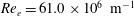 $Re_{e}=61.0\times 10^{6}~\text{m}^{-1}$
). A large-scale STBLI with upstream separation length
$Re_{e}=61.0\times 10^{6}~\text{m}^{-1}$
). A large-scale STBLI with upstream separation length
 ${\sim}30\unicode[STIX]{x1D6FF}_{o}$
(separation to step leading edge) and downstream separation
${\sim}30\unicode[STIX]{x1D6FF}_{o}$
(separation to step leading edge) and downstream separation
 ${\sim}10\unicode[STIX]{x1D6FF}_{o}$
(from step trailing edge) is induced over an axisymmetric configuration and its unsteadiness is characterised by means of time-resolved wall pressure measurements. The extent of the upstream separation matches the typical length of the long coherent structures found in other studies (yet noting the unknowns associated with their scaling), thus putting to test the potential influence of upstream effects related to incoming turbulent fluctuations, which could likely be amplified as they approach a hypothetical resonance of the bubble were they to act as a dominant driving source. The following analysis, however, goes on to suggest otherwise.
${\sim}10\unicode[STIX]{x1D6FF}_{o}$
(from step trailing edge) is induced over an axisymmetric configuration and its unsteadiness is characterised by means of time-resolved wall pressure measurements. The extent of the upstream separation matches the typical length of the long coherent structures found in other studies (yet noting the unknowns associated with their scaling), thus putting to test the potential influence of upstream effects related to incoming turbulent fluctuations, which could likely be amplified as they approach a hypothetical resonance of the bubble were they to act as a dominant driving source. The following analysis, however, goes on to suggest otherwise.
2 Experimental procedures
2.1 Axisymmetric step-induced interaction
The characteristic flow features and organisation of the step-induced STBLI in our study are highlighted in figure 1(a). A fundamental aspect of the geometry lies in its body of revolution configuration as a means to produce an axisymmetric test case – the main appeal of this configuration lying in the high standards of two-dimensionality achieved for the reference flow (yet at the cost of experimental complexity). The incoming boundary layer separates ahead of the step, leading to the formation of a recirculation region of length
 $L_{U}$
upstream of it, which in turn gives rise to an oblique shock wave near separation (
$L_{U}$
upstream of it, which in turn gives rise to an oblique shock wave near separation (
 $S_{1}$
) as the upstream flow is deflected, and to the formation of a detached shock wave close ahead of the step. As the boundary layer goes over the step, it is subjected to a localised expansion over the top lip and a further expansion at the rear lip, respectively indicated as the upstream reattachment
$S_{1}$
) as the upstream flow is deflected, and to the formation of a detached shock wave close ahead of the step. As the boundary layer goes over the step, it is subjected to a localised expansion over the top lip and a further expansion at the rear lip, respectively indicated as the upstream reattachment
 $R_{1}$
and downstream separation
$R_{1}$
and downstream separation
 $S_{2}$
locations. The boundary layer then reattaches further downstream of the step at
$S_{2}$
locations. The boundary layer then reattaches further downstream of the step at
 $R_{2}$
, giving rise to a downstream recirculation of length
$R_{2}$
, giving rise to a downstream recirculation of length
 $L_{D}$
between step back and reattachment. Another oblique shock wave is induced at this location as a result of the local compression experienced by the flow upon reattachment. The respective regions, (
$L_{D}$
between step back and reattachment. Another oblique shock wave is induced at this location as a result of the local compression experienced by the flow upon reattachment. The respective regions, (
 $S_{1}$
–
$S_{1}$
–
 $R_{1}$
) and (
$R_{1}$
) and (
 $S_{2}$
–
$S_{2}$
–
 $R_{2}$
), may be appropriately referred to as two distinct separations, as shown in more detail in § 3. Beyond its canonical approach, this test case thus closely concerns the flow mechanisms induced in regions of surface deflection or off-design imperfection in high-speed vehicles (e.g. panel misalignments, protuberances, etc.) and in part stems from past efforts towards the investigation of the associated local interference effects (Estruch-Samper Reference Estruch-Samper2016).
$R_{2}$
), may be appropriately referred to as two distinct separations, as shown in more detail in § 3. Beyond its canonical approach, this test case thus closely concerns the flow mechanisms induced in regions of surface deflection or off-design imperfection in high-speed vehicles (e.g. panel misalignments, protuberances, etc.) and in part stems from past efforts towards the investigation of the associated local interference effects (Estruch-Samper Reference Estruch-Samper2016).
2.2 Test model and facility
The interaction extends over the measurement length in figure 1(b), where the overall experimental model is shown. The basic test model consists of a stainless steel ogive cylinder body with a base cylinder diameter of
 $D_{B}=75$
mm and nose radius
$D_{B}=75$
mm and nose radius
 $R_{N}=655.7$
mm (nose length
$R_{N}=655.7$
mm (nose length
 $L_{N}=218.6$
mm), aligned axially with the flow at zero incidence. A circumferential step in the form of a disk of diameter
$L_{N}=218.6$
mm), aligned axially with the flow at zero incidence. A circumferential step in the form of a disk of diameter
 $D_{S}=120$
mm is located over the cylindrical section of the body at
$D_{S}=120$
mm is located over the cylindrical section of the body at
 $x_{S}=450$
mm from model nose, with step length
$x_{S}=450$
mm from model nose, with step length
 $l_{S}=22.5$
mm (from step leading to trailing edge); with two further cases with length
$l_{S}=22.5$
mm (from step leading to trailing edge); with two further cases with length
 $2/3l_{S}$
and
$2/3l_{S}$
and
 $1/3l_{S}$
only used later in the paper (in the spectral analysis in § 4) to ascertain that the unsteadiness in the upstream separation is independent of step length. As per figure 1(c), the step height is
$1/3l_{S}$
only used later in the paper (in the spectral analysis in § 4) to ascertain that the unsteadiness in the upstream separation is independent of step length. As per figure 1(c), the step height is
 $h/\unicode[STIX]{x1D6FF}_{o}=5.9$
and the height to length ratio for the case discussed throughout the study is
$h/\unicode[STIX]{x1D6FF}_{o}=5.9$
and the height to length ratio for the case discussed throughout the study is
 $h/l_{S}=1$
. Distinguishing between the upstream and downstream separation regions, the following dimensionless axial locations are defined:
$h/l_{S}=1$
. Distinguishing between the upstream and downstream separation regions, the following dimensionless axial locations are defined:
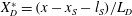
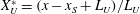 $X_{U}^{\ast }=(x-x_{S}+L_{U})/L_{U}$
and
$X_{U}^{\ast }=(x-x_{S}+L_{U})/L_{U}$
and
 $X_{D}^{\ast }=(x-x_{S}-l_{S})/L_{D}$
, with
$X_{D}^{\ast }=(x-x_{S}-l_{S})/L_{D}$
, with
 $x=0$
taken at nose leading edge. They accordingly provide a measure of their respective dimensionless length
$x=0$
taken at nose leading edge. They accordingly provide a measure of their respective dimensionless length
 $X^{\ast }$
as per equation (1.1). Hence
$X^{\ast }$
as per equation (1.1). Hence
 $X_{U}^{\ast }=0$
and
$X_{U}^{\ast }=0$
and
 $X_{U}^{\ast }=1$
correspond to the locations of upstream separation and step leading edge (
$X_{U}^{\ast }=1$
correspond to the locations of upstream separation and step leading edge (
 $S_{1}$
,
$S_{1}$
,
 $R_{1}$
) and
$R_{1}$
) and
 $X_{D}^{\ast }=0$
and
$X_{D}^{\ast }=0$
and
 $X_{D}^{\ast }=1$
are step trailing edge and downstream reattachment (
$X_{D}^{\ast }=1$
are step trailing edge and downstream reattachment (
 $S_{2}$
,
$S_{2}$
,
 $R_{2}$
).
$R_{2}$
).
Experiments were conducted at the Singapore National Wind Tunnel Facility at a free-stream Mach number of
 $M_{\infty }=3.93$
and unit Reynolds number
$M_{\infty }=3.93$
and unit Reynolds number
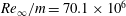 $Re_{\infty }/m=70.1\times 10^{6}$
. This is an intermittent blowdown facility that uses air as the test gas, with typical run durations of 25 s for the present study (test window taken at 15 s from tunnel start) and with a test section of
$Re_{\infty }/m=70.1\times 10^{6}$
. This is an intermittent blowdown facility that uses air as the test gas, with typical run durations of 25 s for the present study (test window taken at 15 s from tunnel start) and with a test section of
 $1.219~\text{m}\times 1.219~\text{m}$
(
$1.219~\text{m}\times 1.219~\text{m}$
(
 $4~\text{ft}\times 4~\text{ft}$
). The free-stream total pressure and total temperature used here are
$4~\text{ft}\times 4~\text{ft}$
). The free-stream total pressure and total temperature used here are
 $P_{o,\infty }=1543$
kPa and
$P_{o,\infty }=1543$
kPa and
 $T_{o,\infty }=308$
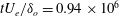
K. The incoming boundary layer is turbulent fully developed and with thickness
$T_{o,\infty }=308$
K. The incoming boundary layer is turbulent fully developed and with thickness
 $\unicode[STIX]{x1D6FF}_{o}=3.8$
mm, at
$\unicode[STIX]{x1D6FF}_{o}=3.8$
mm, at
 $99.5\,\%U_{e}$
where edge velocity is
$99.5\,\%U_{e}$
where edge velocity is
 $U_{e}=683~\text{m}~\text{s}^{-1}$
, as measured through local Pitot tube measurements at the upstream separation location
$U_{e}=683~\text{m}~\text{s}^{-1}$
, as measured through local Pitot tube measurements at the upstream separation location
 $X_{U}^{\ast }=0$
(i.e. at the
$X_{U}^{\ast }=0$
(i.e. at the
 $S_{1}$
reference location but without the step). Test model cross-section with the
$S_{1}$
reference location but without the step). Test model cross-section with the
 $h/\unicode[STIX]{x1D6FF}_{o}=5.9$
step is 0.8 % of the tunnel section and wall temperature is adiabatic (
$h/\unicode[STIX]{x1D6FF}_{o}=5.9$
step is 0.8 % of the tunnel section and wall temperature is adiabatic (
 $T_{w}\approx 284$
K in the reference undisturbed flow), with further relevant flow conditions listed in table 1. The measurement region is comprised within
$T_{w}\approx 284$
K in the reference undisturbed flow), with further relevant flow conditions listed in table 1. The measurement region is comprised within
 $\pm 144$
mm (
$\pm 144$
mm (
 $\pm 38\unicode[STIX]{x1D6FF}_{o}$
) from both sides of the step.
$\pm 38\unicode[STIX]{x1D6FF}_{o}$
) from both sides of the step.
The total pressure
 $P_{o,\infty }$
and temperature
$P_{o,\infty }$
and temperature
 $T_{o,\infty }$
traces for a typical run are given in figure 2 together with the nominal flow conditions in table 1. To maintain mass flow rate
$T_{o,\infty }$
traces for a typical run are given in figure 2 together with the nominal flow conditions in table 1. To maintain mass flow rate
 ${\dot{m}}_{\infty }$
constant during a typical run, the storage tanks feeding the settling chamber are pressurised at 2813 kPa, releasing a total mass flow of
${\dot{m}}_{\infty }$
constant during a typical run, the storage tanks feeding the settling chamber are pressurised at 2813 kPa, releasing a total mass flow of
 ${\sim}14$
tonnes of air over the run duration, approximately 20 % of which flows at
${\sim}14$
tonnes of air over the run duration, approximately 20 % of which flows at
 $529~\text{kg}~\text{s}^{-1}$
over the test window. Upon tunnel start, the total pressure in the test section is shown to rise from ambient conditions and to then rapidly establish; thereafter, total pressure remains highly constant at 1543 kPa
$529~\text{kg}~\text{s}^{-1}$
over the test window. Upon tunnel start, the total pressure in the test section is shown to rise from ambient conditions and to then rapidly establish; thereafter, total pressure remains highly constant at 1543 kPa
 $\pm 0.2\,\%$
and total temperature (in great part compensated through plenum chamber heaters) exhibits a slight decay and remains within 308 K
$\pm 0.2\,\%$
and total temperature (in great part compensated through plenum chamber heaters) exhibits a slight decay and remains within 308 K
 $\pm 1.5\,\%$
over the established flow window (15–20.24 s from tunnel start). As further shown from the computational fluid dynamics (CFD) studies in the following section, the unit Reynolds number at
$\pm 1.5\,\%$
over the established flow window (15–20.24 s from tunnel start). As further shown from the computational fluid dynamics (CFD) studies in the following section, the unit Reynolds number at
 $S_{1}$
based on conditions at boundary-layer edge is
$S_{1}$
based on conditions at boundary-layer edge is
 $Re_{e}/m=61.0\times 10^{6}\pm 3.2\,\%$
. The test model surface (stainless steel) is highly polished and, given the high Reynolds number, the boundary layer is naturally developed to a fully turbulent state.
$Re_{e}/m=61.0\times 10^{6}\pm 3.2\,\%$
. The test model surface (stainless steel) is highly polished and, given the high Reynolds number, the boundary layer is naturally developed to a fully turbulent state.

Figure 2. Free-stream total pressure
 $P_{o,\infty }$
(solid line, left axis), total temperature
$P_{o,\infty }$
(solid line, left axis), total temperature
 $T_{o,\infty }$
(short dashed line, right axis) and mass flow rate
$T_{o,\infty }$
(short dashed line, right axis) and mass flow rate
 ${\dot{m}}_{\infty }$
(long dashed line, right axis) over wind tunnel run. Test window delimited by vertical dashed lines.
${\dot{m}}_{\infty }$
(long dashed line, right axis) over wind tunnel run. Test window delimited by vertical dashed lines.
Table 1. Nominal flow conditions: free-stream Mach number
 $M_{\infty }$
and total pressure
$M_{\infty }$
and total pressure
 $P_{o,\infty }$
; edge Mach number
$P_{o,\infty }$
; edge Mach number
 $M_{e}$
, static temperature
$M_{e}$
, static temperature
 $T_{e}$
, velocity
$T_{e}$
, velocity
 $U_{e}$
and unit Reynolds number
$U_{e}$
and unit Reynolds number
 $Re_{e}/m$
; and boundary-layer thickness
$Re_{e}/m$
; and boundary-layer thickness
 $\unicode[STIX]{x1D6FF}_{o}$
. Reference conditions taken at the axial location corresponding to that of separation
$\unicode[STIX]{x1D6FF}_{o}$
. Reference conditions taken at the axial location corresponding to that of separation
 $S_{1}$
(
$S_{1}$
(
 $X_{U}^{\ast }=0$
) but on the base model only without the step (fully attached flow).
$X_{U}^{\ast }=0$
) but on the base model only without the step (fully attached flow).
2.3 Reference flow conditions
For experimental design purposes, the undisturbed flow conditions on the base ogive cylinder body were estimated using Reynolds-averaged Navier–Stokes (RANS), with the algebraic turbulence model of Baldwin & Lomax (Reference Baldwin and Lomax1978). The numerical procedure – developed by Professor R. Hillier’s group at Imperial College London, Aeronautics Department – is the same as that used in the axisymmetric STBLI studies by Murray, Hillier & Williams (Reference Murray, Hillier and Williams2013); it is here formulated as a second-order accurate ‘convection–diffusion-split’ axisymmetric Navier–Stokes code with convective fluxes solved using an explicit generalised Riemann problem and diffusive fluxes evaluated by an explicit centred-differencing procedure. The grid was structured, with quadrilateral cells, and simulated the complete ogive cylinder model (without step) and with the switch to turbulent flow at
 $x_{tr}=5$
mm from nose leading edge. Three mesh levels were considered, each with successive halving of cell dimensions, and yielding an estimated uncertainty of
$x_{tr}=5$
mm from nose leading edge. Three mesh levels were considered, each with successive halving of cell dimensions, and yielding an estimated uncertainty of
 $\pm 0.2\,\%$
in wall pressure based on the grid independence analysis (
$\pm 0.2\,\%$
in wall pressure based on the grid independence analysis (
 $\pm 0.4\,\%$
accounting for tunnel
$\pm 0.4\,\%$
accounting for tunnel
 $P_{o,\infty }$
uncertainty). The results presented herein correspond to both the coarsest and the finest cases in the study, with
$P_{o,\infty }$
uncertainty). The results presented herein correspond to both the coarsest and the finest cases in the study, with
 $N_{x}\times N_{y}=1301\times 1503$
cells respectively in the streamwise and wall-normal directions for the finest mesh and adaptively refined to
$N_{x}\times N_{y}=1301\times 1503$
cells respectively in the streamwise and wall-normal directions for the finest mesh and adaptively refined to
 $y^{+}=1$
for wall-adjacent cells (with
$y^{+}=1$
for wall-adjacent cells (with
 $N_{x}\times N_{y}=323\times 374$
cells and
$N_{x}\times N_{y}=323\times 374$
cells and
 $y^{+}=4$
for the coarse mesh; and
$y^{+}=4$
for the coarse mesh; and
 $N_{x}\times N_{y}=647\times 747$
cells at
$N_{x}\times N_{y}=647\times 747$
cells at
 $y^{+}=2$
for the medium mesh).
$y^{+}=2$
for the medium mesh).

Figure 3. Reference base flow: pressure (solid lines, left axis), edge Mach number (short dashed lines, right axis) and Reynolds number (long dashed lines, right axis) along streamwise direction and with reference to respective free-stream values (
 $p/p_{\infty }$
,
$p/p_{\infty }$
,
 $M_{e}/M_{\infty }$
and
$M_{e}/M_{\infty }$
and
 $Re_{e}/Re_{\infty }$
) based on turbulent CFD using the Baldwin–Lomax model (
$Re_{e}/Re_{\infty }$
) based on turbulent CFD using the Baldwin–Lomax model (
 $N_{x}\times N_{y}=1301\times 1500$
,
$N_{x}\times N_{y}=1301\times 1500$
,
 $y^{+}=1$
for fine-resolution mesh in black;
$y^{+}=1$
for fine-resolution mesh in black;
 $N_{x}\times N_{y}=323\times 374$
,
$N_{x}\times N_{y}=323\times 374$
,
 $y^{+}=4$
for coarse mesh in grey). Medium case (
$y^{+}=4$
for coarse mesh in grey). Medium case (
 $N_{x}\times N_{y}=647\times 747$
,
$N_{x}\times N_{y}=647\times 747$
,
 $y^{+}=2$
) falls in between but is not shown for illustration purposes. Grey square at the bottom indicates the location where the step is subsequently placed (no step considered in the CFD shown here) and vertical dashed lines delimit the measurement region.
$y^{+}=2$
) falls in between but is not shown for illustration purposes. Grey square at the bottom indicates the location where the step is subsequently placed (no step considered in the CFD shown here) and vertical dashed lines delimit the measurement region.
As shown in the CFD solutions in figure 3, following the compression across the oblique shock wave at the nose leading edge, the static pressure at the wall drops along the nose length to then gradually approach the free-stream levels over the cylindrical section, with edge Reynolds number exhibiting a similar trend and establishing at approximately 15 % below that in the free stream (
 ${\sim}0.87Re_{\infty }$
). The Mach number at the boundary-layer edge instead rises gradually along the nose length as it recovers from the deceleration across the shock and establishes near the free-stream levels, subsequently adopting a weak adverse gradient over the measurement region (
${\sim}0.87Re_{\infty }$
). The Mach number at the boundary-layer edge instead rises gradually along the nose length as it recovers from the deceleration across the shock and establishes near the free-stream levels, subsequently adopting a weak adverse gradient over the measurement region (
 $\unicode[STIX]{x0394}M=-0.076$
). The corresponding pressure and Reynolds number variations over the same region, and inherent to the axisymmetric configuration, are
$\unicode[STIX]{x0394}M=-0.076$
). The corresponding pressure and Reynolds number variations over the same region, and inherent to the axisymmetric configuration, are
 $\unicode[STIX]{x0394}p=1096$
Pa and
$\unicode[STIX]{x0394}p=1096$
Pa and
 $\unicode[STIX]{x0394}Re=2.9\times 10^{6}~\text{m}^{-1}$
. Along the upstream separation length
$\unicode[STIX]{x0394}Re=2.9\times 10^{6}~\text{m}^{-1}$
. Along the upstream separation length
 $L_{U}$
(
$L_{U}$
(
 ${\sim}30\unicode[STIX]{x1D6FF}_{o}$
), the respective variations are
${\sim}30\unicode[STIX]{x1D6FF}_{o}$
), the respective variations are
 $-0.7\,\%M_{e}$
,
$-0.7\,\%M_{e}$
,
 $+3.6\,\%p_{\infty }$
and
$+3.6\,\%p_{\infty }$
and
 $+1.5\,\%Re_{e}$
. The axial pressure gradient (
$+1.5\,\%Re_{e}$
. The axial pressure gradient (
 $\text{d}p/\text{d}x$
) was found to be negligible over the cylindrical section of the body so that the base turbulent boundary layer is thus at equilibrium.
$\text{d}p/\text{d}x$
) was found to be negligible over the cylindrical section of the body so that the base turbulent boundary layer is thus at equilibrium.
As earlier noted, the reference (undisturbed) boundary-layer profile was experimentally measured through Pitot tube measurements. The Pitot tube head had an inlet area of
 ${\sim}0.8~\text{mm}^{2}$
(2 mm-wide by 0.4 mm-high) and was adjusted in
${\sim}0.8~\text{mm}^{2}$
(2 mm-wide by 0.4 mm-high) and was adjusted in
 $\unicode[STIX]{x0394}y=0.2$
mm (
$\unicode[STIX]{x0394}y=0.2$
mm (
 $\pm 1.3\,\%$
) steps between runs, covering a sufficient range above the boundary-layer edge and down to 0.6 mm from the wall, below which measurements were not feasible due to strong interference. The probe was positioned to measure at a location corresponding to upstream separation
$\pm 1.3\,\%$
) steps between runs, covering a sufficient range above the boundary-layer edge and down to 0.6 mm from the wall, below which measurements were not feasible due to strong interference. The probe was positioned to measure at a location corresponding to upstream separation
 $S_{1}$
, i.e.
$S_{1}$
, i.e.
 $X_{U}^{\ast }=0$
(again noting no step was used in order to characterise the local undisturbed boundary layer). The velocity and Mach number profiles in figure 4 are thus derived through Rayleigh–Pitot theory and assume constant total temperature and static pressure at the measurement station. The reference (undisturbed) boundary layer is shown to comply with a turbulent profile with thickness
$X_{U}^{\ast }=0$
(again noting no step was used in order to characterise the local undisturbed boundary layer). The velocity and Mach number profiles in figure 4 are thus derived through Rayleigh–Pitot theory and assume constant total temperature and static pressure at the measurement station. The reference (undisturbed) boundary layer is shown to comply with a turbulent profile with thickness
 $\unicode[STIX]{x1D6FF}_{o}=3.8$
mm (
$\unicode[STIX]{x1D6FF}_{o}=3.8$
mm (
 $99.5\,\%U_{e}$
). As shown in the figure, the experimental results are in close agreement with the CFD, both approximately following a one-seventh power-law velocity profile,
$99.5\,\%U_{e}$
). As shown in the figure, the experimental results are in close agreement with the CFD, both approximately following a one-seventh power-law velocity profile,
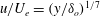 $u/U_{e}=(y/\unicode[STIX]{x1D6FF}_{o})^{1/7}$
. The Mach number profile is also as expected for an equilibrium high Mach turbulent boundary layer (e.g. as per Duan, Choudhari & Zhang Reference Duan, Choudhari and Zhang2016).
$u/U_{e}=(y/\unicode[STIX]{x1D6FF}_{o})^{1/7}$
. The Mach number profile is also as expected for an equilibrium high Mach turbulent boundary layer (e.g. as per Duan, Choudhari & Zhang Reference Duan, Choudhari and Zhang2016).

Figure 4. Incoming boundary-layer profile: (a) streamwise velocity
 $u$
and (b) Mach number
$u$
and (b) Mach number
 $M$
at reference separation location
$M$
at reference separation location
 $S_{1}$
, corresponding to
$S_{1}$
, corresponding to
 $X_{U}^{\ast }=0$
but without the step (base cylinder only). Experimental Pitot tube measurements respectively as square and diamond symbols; and numerical predictions as solid black lines; with one-seventh power-law velocity profile (long dashed line),
$X_{U}^{\ast }=0$
but without the step (base cylinder only). Experimental Pitot tube measurements respectively as square and diamond symbols; and numerical predictions as solid black lines; with one-seventh power-law velocity profile (long dashed line),
 $u/U_{e}=(y/\unicode[STIX]{x1D6FF}_{o})^{1/7}$
. Free-stream conditions:
$u/U_{e}=(y/\unicode[STIX]{x1D6FF}_{o})^{1/7}$
. Free-stream conditions:
 $p_{\infty }=11\,161$
Pa,
$p_{\infty }=11\,161$
Pa,
 $Re_{\infty }=71\times 10^{6}~\text{m}^{-1}$
and
$Re_{\infty }=71\times 10^{6}~\text{m}^{-1}$
and
 $M_{\infty }=3.93$
.
$M_{\infty }=3.93$
.
2.4 Time-resolved pressure measurements
Fast response piezoresistive silicon pressure transducers of the type Kulite XCQ-055 (rated at 25 psi absolute and with a natural frequency of 210 kHz) were set in instrumentation modules on both sides of the step and flush to the model surface, as per the schematic in figure 5(a). The output of the 32 sensors was digitised simultaneously at a sampling rate of
 $200~\text{kS}~\text{s}^{-1}$
per channel at 24-bit (DeweSoft SIRIUSi system) with a cutoff frequency of 100 kHz. The sensors were selected due to their combined high-frequency and ‘ultraminiature’ size, which offered the best trade-off for the study in terms of both spatial and spectral resolution considerations (higher-frequency sensors more often used for shock passage and vibration measurements were deemed less suitable for the present purposes). The sensor design relies on a thin screen (Kulite ‘b-screen’) which, as sketched in figure 5(b), is composed of eight 0.15 mm-diameter orifices arranged in a circular pattern of diameter
$200~\text{kS}~\text{s}^{-1}$
per channel at 24-bit (DeweSoft SIRIUSi system) with a cutoff frequency of 100 kHz. The sensors were selected due to their combined high-frequency and ‘ultraminiature’ size, which offered the best trade-off for the study in terms of both spatial and spectral resolution considerations (higher-frequency sensors more often used for shock passage and vibration measurements were deemed less suitable for the present purposes). The sensor design relies on a thin screen (Kulite ‘b-screen’) which, as sketched in figure 5(b), is composed of eight 0.15 mm-diameter orifices arranged in a circular pattern of diameter
 $d_{\unicode[STIX]{x1D705},1}=0.87$
mm (sensor outer diameter being
$d_{\unicode[STIX]{x1D705},1}=0.87$
mm (sensor outer diameter being
 $d_{\unicode[STIX]{x1D705},2}=1.40$
mm), with the associated spatial resolution corresponding to 0.75 % of the upstream separation length
$d_{\unicode[STIX]{x1D705},2}=1.40$
mm), with the associated spatial resolution corresponding to 0.75 % of the upstream separation length
 $L_{U}$
(further details in § 3). Overall, sensors were spaced at
$L_{U}$
(further details in § 3). Overall, sensors were spaced at
 $\unicode[STIX]{x1D709}=4.5$
mm in the streamwise direction, starting 2.25 mm from both sides of the step, i.e. at
$\unicode[STIX]{x1D709}=4.5$
mm in the streamwise direction, starting 2.25 mm from both sides of the step, i.e. at
 $\unicode[STIX]{x0394}X_{U}^{\ast }=0.04$
between sensors. Alternate instrumentation arrangements were used to cover longer extents in the axial direction (
$\unicode[STIX]{x0394}X_{U}^{\ast }=0.04$
between sensors. Alternate instrumentation arrangements were used to cover longer extents in the axial direction (
 $\unicode[STIX]{x1D709}=9$
mm) for correlation purposes as well as for azimuthal measurements (
$\unicode[STIX]{x1D709}=9$
mm) for correlation purposes as well as for azimuthal measurements (
 $\unicode[STIX]{x0394}\unicode[STIX]{x1D711}=6.5$
mm) at selected locations.
$\unicode[STIX]{x0394}\unicode[STIX]{x1D711}=6.5$
mm) at selected locations.

Figure 5. Schematics of fast response pressure sensor (Kulite XCQ-055, 210 kHz natural frequency) instrumented module indicating: (a) side view of sensor (A), test model surface (B), in-house sensor protective casing (C), epoxy (D) and (b) plan view indicating spacing between sensors
 $\unicode[STIX]{x1D709}=4.5$
mm (9 mm for upstream/downstream correlation purposes), sensor casing (E) and sensor tappings (F). Sensor outer diameter is
$\unicode[STIX]{x1D709}=4.5$
mm (9 mm for upstream/downstream correlation purposes), sensor casing (E) and sensor tappings (F). Sensor outer diameter is
 $d_{K1}=1.40$
mm and circular 8-orifice arrangements (diameter
$d_{K1}=1.40$
mm and circular 8-orifice arrangements (diameter
 $d_{K2}=0.87$
mm) indicate the pressure sensor tapings (individual taping diameter 0.15 mm). Kulite sensors placed flush (within
$d_{K2}=0.87$
mm) indicate the pressure sensor tapings (individual taping diameter 0.15 mm). Kulite sensors placed flush (within
 $\pm 0.1$
mm accuracy) to test model surface.
$\pm 0.1$
mm accuracy) to test model surface.
Unsteady data analysis considers test windows with a total duration of 5.24 s (15–20.24 s from tunnel start) and spectral quantities are obtained by ensemble averaging 64 blocks of
 $2^{14}$
samples at 50 % overlap (with Welch’s method, Hanning window) yielding a frequency resolution of
$2^{14}$
samples at 50 % overlap (with Welch’s method, Hanning window) yielding a frequency resolution of
 $\unicode[STIX]{x0394}f=12.2$
Hz. The total error associated with the pressure measurements, accounting for sensor calibration, system error and testing conditions is
$\unicode[STIX]{x0394}f=12.2$
Hz. The total error associated with the pressure measurements, accounting for sensor calibration, system error and testing conditions is
 $\pm 2\,\%$
. To ensure axisymmetry, mean pressure measurements were simultaneously obtained in the axial direction on the opposite side of the cylinder, using 32 piezoresistive pressure sensors (ESP transducers rated at 30 psi and sampled at 50 Hz), within 0.8 % uncertainty. High-speed schlieren images were also simultaneously obtained using a Photron SA-X2 camera.
$\pm 2\,\%$
. To ensure axisymmetry, mean pressure measurements were simultaneously obtained in the axial direction on the opposite side of the cylinder, using 32 piezoresistive pressure sensors (ESP transducers rated at 30 psi and sampled at 50 Hz), within 0.8 % uncertainty. High-speed schlieren images were also simultaneously obtained using a Photron SA-X2 camera.
Samples of the time-dependent pressure traces are presented in figure 6, corresponding to the following characteristic locations along the interaction: the upstream separation location
 $X_{U}^{\ast }=0$
, near the corner just ahead of the step
$X_{U}^{\ast }=0$
, near the corner just ahead of the step
 $X_{U}^{\ast }=0.98$
(with increased mean pressure levels) and the downstream reattachment location
$X_{U}^{\ast }=0.98$
(with increased mean pressure levels) and the downstream reattachment location
 $X_{D}^{\ast }=1$
(lower pressure following the flow’s expansion over the step). The panels zoom into different periods within the run. Figure 6(a) starts with the complete test run and captures the drop from ambient to free-stream pressure upon tunnel start. In figure 6(b), the test window between 15–20.54 s (
$X_{D}^{\ast }=1$
(lower pressure following the flow’s expansion over the step). The panels zoom into different periods within the run. Figure 6(a) starts with the complete test run and captures the drop from ambient to free-stream pressure upon tunnel start. In figure 6(b), the test window between 15–20.54 s (
 $tU_{e}/\unicode[STIX]{x1D6FF}_{o}=0.94\times 10^{6}$
) from start is shown, capturing the complete signal duration upon which the unsteady data analysis relies. Close ups into 0.5-second (
$tU_{e}/\unicode[STIX]{x1D6FF}_{o}=0.94\times 10^{6}$
) from start is shown, capturing the complete signal duration upon which the unsteady data analysis relies. Close ups into 0.5-second (
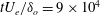 $tU_{e}/\unicode[STIX]{x1D6FF}_{o}=9\times 10^{4}$
) and 0.1-second periods (
$tU_{e}/\unicode[STIX]{x1D6FF}_{o}=9\times 10^{4}$
) and 0.1-second periods (
 $tU_{e}/\unicode[STIX]{x1D6FF}_{o}=1.8\times 10^{4}$
), from beginning of test window, are accordingly shown in figure 6(c,d).
$tU_{e}/\unicode[STIX]{x1D6FF}_{o}=1.8\times 10^{4}$
), from beginning of test window, are accordingly shown in figure 6(c,d).

Figure 6. Sample time-dependent static pressure traces at locations of separation
 $X_{U}^{\ast }=0$
(red), corner
$X_{U}^{\ast }=0$
(red), corner
 $X_{U}^{\ast }=0.98$
(green) and downstream reattachment
$X_{U}^{\ast }=0.98$
(green) and downstream reattachment
 $X_{D}^{\ast }=1$
(blue) zooming into different periods: (a) complete test run including tunnel start, (b) test window for present study (15–20.54 s from start), (c) zoom into 0.5 s-period (
$X_{D}^{\ast }=1$
(blue) zooming into different periods: (a) complete test run including tunnel start, (b) test window for present study (15–20.54 s from start), (c) zoom into 0.5 s-period (
 $tU_{e}/\unicode[STIX]{x1D6FF}_{o}=9\times 10^{4}$
) from beginning of test window, (d) zoom into 0.1 s-period (
$tU_{e}/\unicode[STIX]{x1D6FF}_{o}=9\times 10^{4}$
) from beginning of test window, (d) zoom into 0.1 s-period (
 $tU_{e}/\unicode[STIX]{x1D6FF}_{o}=1.8\times 10^{4}$
) from beginning of test window. Horizontal dashed line marks free-stream pressure level of
$tU_{e}/\unicode[STIX]{x1D6FF}_{o}=1.8\times 10^{4}$
) from beginning of test window. Horizontal dashed line marks free-stream pressure level of
 $p_{\infty }=11161$
Pa.
$p_{\infty }=11161$
Pa.

Figure 7. Highly separated axisymmetric step STBLI, induced by
 $h/\unicode[STIX]{x1D6FF}_{o}=5.9$
step: (a) sample of time-dependent pressure at different locations along separation, (b) schlieren image of overall measurement region, excluding attached shock region over nose leading edge (Z-type optical arrangement with concave mirrors of diameter
$h/\unicode[STIX]{x1D6FF}_{o}=5.9$
step: (a) sample of time-dependent pressure at different locations along separation, (b) schlieren image of overall measurement region, excluding attached shock region over nose leading edge (Z-type optical arrangement with concave mirrors of diameter
 $\varnothing =0.5$
m, focal length
$\varnothing =0.5$
m, focal length
 $f=6$
m) and (c) mean pressure in the axial direction
$f=6$
m) and (c) mean pressure in the axial direction
 $p$
(black diamond symbols, left axis) and relative standard deviation
$p$
(black diamond symbols, left axis) and relative standard deviation
 $\unicode[STIX]{x1D70E}_{p}/p$
(grey squares, right axis). Labels a–f correspond to distinctive regions along STBLI, respectively: upstream separation, rise to plateau, ahead of step, behind step, downstream reattachment and relaxation regions. Empty diamond symbols (♢) indicate mean pressure at the opposite side of the model (
$\unicode[STIX]{x1D70E}_{p}/p$
(grey squares, right axis). Labels a–f correspond to distinctive regions along STBLI, respectively: upstream separation, rise to plateau, ahead of step, behind step, downstream reattachment and relaxation regions. Empty diamond symbols (♢) indicate mean pressure at the opposite side of the model (
 $\unicode[STIX]{x1D719}=180^{\circ }$
). Intermittency at
$\unicode[STIX]{x1D719}=180^{\circ }$
). Intermittency at
 $X_{U}^{\ast }=0$
is
$X_{U}^{\ast }=0$
is
 $\unicode[STIX]{x1D6FE}=0.2$
, where
$\unicode[STIX]{x1D6FE}=0.2$
, where
 $\unicode[STIX]{x1D6FE}=(p_{x}-p_{u})/(p_{pu}-p_{u})$
and normalised standard deviation
$\unicode[STIX]{x1D6FE}=(p_{x}-p_{u})/(p_{pu}-p_{u})$
and normalised standard deviation
 $\unicode[STIX]{x1D70E}/p_{x}=0.28$
(local pressure
$\unicode[STIX]{x1D70E}/p_{x}=0.28$
(local pressure
 $p_{x}=13\,930$
Pa).
$p_{x}=13\,930$
Pa).
3 Highly separated interaction
3.1 Flow organisation
The strongly oscillatory behaviour of the flow along the upstream separation region is evidenced in more detail in the time-dependent pressure traces in figure 7(a). Qualitative details on the flow organisation for the overall cylinder/disk configuration can be further found in the schlieren image in figure 7(b). The oblique shock wave induced upon separation – intrinsically associated with the large-amplitude oscillations in wall pressure – appears particularly well defined and is followed by a long separation region on the two opposite sides of the model imaged here, i.e. given the axisymmetric separation extends around the azimuthal direction (cylinder perimeter). The sample measurements in figure 7(a) document the pressure rise along separation and capture the progressive variation in the flow’s intermittent behaviour within this region. The signal at
 $X_{U}^{\ast }=-0.04$
, just upstream of separation, starts to exhibit occasional excursions in pressure as the oblique separation shock reaches this location. This effect becomes particularly notable at
$X_{U}^{\ast }=-0.04$
, just upstream of separation, starts to exhibit occasional excursions in pressure as the oblique separation shock reaches this location. This effect becomes particularly notable at
 $X_{U}^{\ast }=0$
, where the signal oscillates drastically between the base pressure and up to above twice a higher level (longer samples of the same pressure trace may be found in figure 6). By
$X_{U}^{\ast }=0$
, where the signal oscillates drastically between the base pressure and up to above twice a higher level (longer samples of the same pressure trace may be found in figure 6). By
 $X_{U}^{\ast }=0.12$
, downstream of separation, the pressure is approaching the plateau level and no longer exhibits large-amplitude oscillations.
$X_{U}^{\ast }=0.12$
, downstream of separation, the pressure is approaching the plateau level and no longer exhibits large-amplitude oscillations.
In figure 7(c), the mean pressure results are shown overlapped with the relative standard deviation maxima
 $(\unicode[STIX]{x1D70E}_{p}/p)_{max}$
– the local maxima for the latter serving to identify the upstream separation
$(\unicode[STIX]{x1D70E}_{p}/p)_{max}$
– the local maxima for the latter serving to identify the upstream separation
 $S_{1}$
and downstream reattachment locations
$S_{1}$
and downstream reattachment locations
 $R_{2}$
(note again the large-scale oscillations at
$R_{2}$
(note again the large-scale oscillations at
 $X_{U}^{\ast }=0$
and
$X_{U}^{\ast }=0$
and
 $X_{D}^{\ast }=1$
in figure 6). The upstream pressure exhibits a first rise from the base undisturbed level of
$X_{D}^{\ast }=1$
in figure 6). The upstream pressure exhibits a first rise from the base undisturbed level of
 $p_{u}=9.84$
kPa slightly ahead of separation
$p_{u}=9.84$
kPa slightly ahead of separation
 $S_{1}$
towards a plateau level of approximately
$S_{1}$
towards a plateau level of approximately
 $p_{p,U}\approx 28$
kPa (
$p_{p,U}\approx 28$
kPa (
 ${\sim}2.85p_{u}$
), which is then followed by a further overshoot to
${\sim}2.85p_{u}$
), which is then followed by a further overshoot to
 ${\sim}35.8$
kPa (3.64
${\sim}35.8$
kPa (3.64
 $p_{u}$
), as measured at 2.25 mm upstream of the step (
$p_{u}$
), as measured at 2.25 mm upstream of the step (
 $X_{U}^{\ast }=0.98$
). Following the flow’s expansion over the step, the pressure within the downstream recirculation is found to increase from a plateau level of around
$X_{U}^{\ast }=0.98$
). Following the flow’s expansion over the step, the pressure within the downstream recirculation is found to increase from a plateau level of around
 $p_{p,D}=2.28$
kPa (0.23
$p_{p,D}=2.28$
kPa (0.23
 $p_{u}$
) to eventually return to the undisturbed levels. The upstream and downstream separation lengths are respectively
$p_{u}$
) to eventually return to the undisturbed levels. The upstream and downstream separation lengths are respectively
 $L_{U}=114.75~\text{mm}\pm 4\,\%$
(30.2
$L_{U}=114.75~\text{mm}\pm 4\,\%$
(30.2
 $\unicode[STIX]{x1D6FF}_{o}$
) and
$\unicode[STIX]{x1D6FF}_{o}$
) and
 $L_{D}=38.25~\text{mm}\pm 12\,\%$
(10.1
$L_{D}=38.25~\text{mm}\pm 12\,\%$
(10.1
 $\unicode[STIX]{x1D6FF}_{o}$
). The following regions may thus be highlighted as per the labels in the figure: (a) marks the first pressure rise starting just ahead of separation as associated with the separation shock, in (b) the plateau level is found from approximately
$\unicode[STIX]{x1D6FF}_{o}$
). The following regions may thus be highlighted as per the labels in the figure: (a) marks the first pressure rise starting just ahead of separation as associated with the separation shock, in (b) the plateau level is found from approximately
 $X_{U}^{\ast }=0.20$
and extending along the upstream recirculation region, (c) indicates the second pressure overshoot at
$X_{U}^{\ast }=0.20$
and extending along the upstream recirculation region, (c) indicates the second pressure overshoot at
 $X_{U}^{\ast }\approx 0.90$
, associated with the local detached shock, (d) shows a plateau extending to
$X_{U}^{\ast }\approx 0.90$
, associated with the local detached shock, (d) shows a plateau extending to
 $X_{D}^{\ast }=0.65$
within the recirculation region behind the step, (e) marks a recompression region along reattachment associated with the downstream reattachment shock and (f) a relaxation region that eventually leads to the flow’s recovery far downstream of the interaction.
$X_{D}^{\ast }=0.65$
within the recirculation region behind the step, (e) marks a recompression region along reattachment associated with the downstream reattachment shock and (f) a relaxation region that eventually leads to the flow’s recovery far downstream of the interaction.
A sequence of axial pressure and simultaneous schlieren images is presented in figure 8 to highlight the transient contraction and expansion of the upstream separation region. The sequence spans 3.4 ms (
 $tU_{e}/\unicode[STIX]{x1D6FF}_{o}=611$
) and captures a period in excess of that for a typical oscillation of the upstream separation shock (§ 3.4). At the start of the sequence, the pressure rise upon separation is found to shift downstream as the shock moves towards the step (refer to the
$tU_{e}/\unicode[STIX]{x1D6FF}_{o}=611$
) and captures a period in excess of that for a typical oscillation of the upstream separation shock (§ 3.4). At the start of the sequence, the pressure rise upon separation is found to shift downstream as the shock moves towards the step (refer to the
 $p/p_{u}$
ratios in the right axis of the figure); subsequently, the shock wave then returns to its original location and shifts further upstream as the separation bubble is enlarged. The process appears to then proceed again with a further contraction of the bubble in this instance. The pressure over the plateau region is noted to be approximately at the plateau level ahead of the step, within the intrinsically irregular turbulent events. It may be seen that, at times, the pressure close upstream of the step overshoots significantly above the local mean, while in other instances the plateau is extended all the way down to
$p/p_{u}$
ratios in the right axis of the figure); subsequently, the shock wave then returns to its original location and shifts further upstream as the separation bubble is enlarged. The process appears to then proceed again with a further contraction of the bubble in this instance. The pressure over the plateau region is noted to be approximately at the plateau level ahead of the step, within the intrinsically irregular turbulent events. It may be seen that, at times, the pressure close upstream of the step overshoots significantly above the local mean, while in other instances the plateau is extended all the way down to
 $X_{U}^{\ast }=0.98$
(just ahead of the step). The sample is here shown to highlight a characteristic oscillation of the interaction but a closer look into longer periods clearly finds that the contraction–expansion cycle is not precisely repeated over time. More details on interaction unsteadiness are thus to be derived through spectral analysis (in § 3.3). Prior to that, further characterisation of the upstream flow effects is provided next.
$X_{U}^{\ast }=0.98$
(just ahead of the step). The sample is here shown to highlight a characteristic oscillation of the interaction but a closer look into longer periods clearly finds that the contraction–expansion cycle is not precisely repeated over time. More details on interaction unsteadiness are thus to be derived through spectral analysis (in § 3.3). Prior to that, further characterisation of the upstream flow effects is provided next.

Figure 8. Sequence of axial pressure (black square symbols) over the interaction region upstream of the step together with simultaneous schlieren images, over a 3.4 ms period (
 $tU_{e}/\unicode[STIX]{x1D6FF}_{o}=611$
); shown at
$tU_{e}/\unicode[STIX]{x1D6FF}_{o}=611$
); shown at
 $\unicode[STIX]{x0394}t=0.2$
ms time steps (
$\unicode[STIX]{x0394}t=0.2$
ms time steps (
 $\unicode[STIX]{x0394}tU_{e}/\unicode[STIX]{x1D6FF}_{o}=36$
). Schlieren images not to scale with image axis. White diamond symbols correspond to the mean pressure measurements (i.e. as per figure 7
c). Vertical dashed lines fixed at
$\unicode[STIX]{x0394}tU_{e}/\unicode[STIX]{x1D6FF}_{o}=36$
). Schlieren images not to scale with image axis. White diamond symbols correspond to the mean pressure measurements (i.e. as per figure 7
c). Vertical dashed lines fixed at
 $X_{U}^{\ast }=0$
in both pressure and schlieren.
$X_{U}^{\ast }=0$
in both pressure and schlieren.
3.2 Incoming turbulent boundary layer
The characteristic large-scale pulsations of the separation bubble are generally regarded as the low frequencies within STBLIs given they are typically approximately two to three orders of magnitude lower than the undisturbed boundary-layer time scales
 $St_{\unicode[STIX]{x1D6FF}}\approx$
 $O(10^{-3}{-}10^{-2})$
, where
$O(10^{-3}{-}10^{-2})$
, where
 $St_{\unicode[STIX]{x1D6FF}}=f\unicode[STIX]{x1D6FF}_{o}/U_{e}$
. While fast response sensors are well suited for measurements of high-speed separated flows, their capabilities are challenged at the high-frequency end of the spectrum, as is often the case when documenting the undisturbed boundary layer. The characteristic time scales of the incoming boundary layer – expectedly having significant spectral content at approximately
$St_{\unicode[STIX]{x1D6FF}}=f\unicode[STIX]{x1D6FF}_{o}/U_{e}$
. While fast response sensors are well suited for measurements of high-speed separated flows, their capabilities are challenged at the high-frequency end of the spectrum, as is often the case when documenting the undisturbed boundary layer. The characteristic time scales of the incoming boundary layer – expectedly having significant spectral content at approximately
 $f\approx U_{e}/\unicode[STIX]{x1D6FF}_{o}$
, more directly associated with energetic eddies – would here be of order
$f\approx U_{e}/\unicode[STIX]{x1D6FF}_{o}$
, more directly associated with energetic eddies – would here be of order
 ${\sim}180$
kHz and hence well above sensor frequency response (the cutoff frequency is effectively
${\sim}180$
kHz and hence well above sensor frequency response (the cutoff frequency is effectively
 $f_{c}\approx 50$
kHz as shown in the following figure). As earlier mentioned in § 2.4, sensors with wider spectral range are on the other hand limited by poor resolution at low pressures and their larger measurement size (roughly 5 times a greater sensing area for 0.5–1 MHz sensors) thus being even further challenged for the measurement of fine-scale high-frequency disturbances. When compared with the turbulent boundary layer dataset evaluated in Beresh et al. (Reference Beresh, Henfling, Spillers and Pruett2011), the normalised standard deviation of the undisturbed wall pressure signal is found to fall at the bottom of the range at
$f_{c}\approx 50$
kHz as shown in the following figure). As earlier mentioned in § 2.4, sensors with wider spectral range are on the other hand limited by poor resolution at low pressures and their larger measurement size (roughly 5 times a greater sensing area for 0.5–1 MHz sensors) thus being even further challenged for the measurement of fine-scale high-frequency disturbances. When compared with the turbulent boundary layer dataset evaluated in Beresh et al. (Reference Beresh, Henfling, Spillers and Pruett2011), the normalised standard deviation of the undisturbed wall pressure signal is found to fall at the bottom of the range at
 $\unicode[STIX]{x1D70E}_{p}/q_{e}\approx 0.001$
(
$\unicode[STIX]{x1D70E}_{p}/q_{e}\approx 0.001$
(
 $\unicode[STIX]{x1D70E}_{p}/\unicode[STIX]{x1D70F}_{w}\approx 1.1$
), where
$\unicode[STIX]{x1D70E}_{p}/\unicode[STIX]{x1D70F}_{w}\approx 1.1$
), where
 $q_{e}$
is dynamic pressure and
$q_{e}$
is dynamic pressure and
 $\unicode[STIX]{x1D70F}_{w}$
is wall shear stress. Spatial resolution in terms of
$\unicode[STIX]{x1D70F}_{w}$
is wall shear stress. Spatial resolution in terms of
 $\unicode[STIX]{x1D714}d/2U_{c}$
, where
$\unicode[STIX]{x1D714}d/2U_{c}$
, where
 $\unicode[STIX]{x1D714}$
is angular frequency and the convection velocity of near-wall structures is approximated by
$\unicode[STIX]{x1D714}$
is angular frequency and the convection velocity of near-wall structures is approximated by
 $U_{c}\approx 0.6U_{e}$
, suggests minimal attenuation of energy scales much smaller than sensor size across the effective 0–50 kHz range and up to approximately 93 kHz (
$U_{c}\approx 0.6U_{e}$
, suggests minimal attenuation of energy scales much smaller than sensor size across the effective 0–50 kHz range and up to approximately 93 kHz (
 $-3$
dB point at
$-3$
dB point at
 $\unicode[STIX]{x1D714}d_{\unicode[STIX]{x1D705},2}/2U_{c}=1$
, as per Corcos (Reference Corcos1963)). The influence of wind tunnel noise and vibration at low frequencies were further assessed through comparison of the present signal with that using an adaptive filter technique as per Naguib, Gravante & Wark (Reference Naguib, Gravante and Wark1996). In relation to the fluctuations associated with the interaction, such an influence was deemed negligible for the present case and hence this conditioning is not applied here.
$\unicode[STIX]{x1D714}d_{\unicode[STIX]{x1D705},2}/2U_{c}=1$
, as per Corcos (Reference Corcos1963)). The influence of wind tunnel noise and vibration at low frequencies were further assessed through comparison of the present signal with that using an adaptive filter technique as per Naguib, Gravante & Wark (Reference Naguib, Gravante and Wark1996). In relation to the fluctuations associated with the interaction, such an influence was deemed negligible for the present case and hence this conditioning is not applied here.
Bearing in mind the above-mentioned limitations, a sample power spectral density of the signal (PSD) of the incoming boundary layer is presented in figure 9(a). To further document the reference flow, measurements were obtained with an in-house ‘high-frequency Pitot tube’ using one of the XCQ-055 Kulite sensors facing the free stream (probe head diameter 1.4 mm, with sensor held protruding off the probe). The sensor was centred at a height of
 $y=2.4$
mm from the wall, with its head covering a region
$y=2.4$
mm from the wall, with its head covering a region
 $y=(0.68\pm 0.18)\unicode[STIX]{x1D6FF}_{o}$
, again at the location corresponding to
$y=(0.68\pm 0.18)\unicode[STIX]{x1D6FF}_{o}$
, again at the location corresponding to
 $X_{U}^{\ast }=0$
but without the step on the model. With further consideration of the wall pressure spectra at the same location, and for both cases, fluctuation energy remains broadband and at a flat level across the low-frequency range (
$X_{U}^{\ast }=0$
but without the step on the model. With further consideration of the wall pressure spectra at the same location, and for both cases, fluctuation energy remains broadband and at a flat level across the low-frequency range (
 $\unicode[STIX]{x1D714}\rightarrow 0$
). Thereafter, the spectra adopt an
$\unicode[STIX]{x1D714}\rightarrow 0$
). Thereafter, the spectra adopt an
 $\unicode[STIX]{x1D714}^{-1}$
trend, with an onset captured at higher frequencies in the Pitot results (and an overshoot at the higher end presumably towards
$\unicode[STIX]{x1D714}^{-1}$
trend, with an onset captured at higher frequencies in the Pitot results (and an overshoot at the higher end presumably towards
 $St_{\unicode[STIX]{x1D6FF}}\approx 1$
). Both the broadband levels at the lower-frequency range (cf. the
$St_{\unicode[STIX]{x1D6FF}}\approx 1$
). Both the broadband levels at the lower-frequency range (cf. the
 $\unicode[STIX]{x1D714}^{2}$
dependence found in a number of incompressible flow studies) and the
$\unicode[STIX]{x1D714}^{2}$
dependence found in a number of incompressible flow studies) and the
 $\unicode[STIX]{x1D714}^{-1}$
are consistent with the high-speed flow experiments in Beresh et al. (Reference Beresh, Henfling, Spillers and Pruett2011) and Casper, Beresh & Schneider (Reference Casper, Beresh and Schneider2014), as well as the DNS by Duan et al. (Reference Duan, Choudhari and Zhang2016). As similarly found in these studies, the
$\unicode[STIX]{x1D714}^{-1}$
are consistent with the high-speed flow experiments in Beresh et al. (Reference Beresh, Henfling, Spillers and Pruett2011) and Casper, Beresh & Schneider (Reference Casper, Beresh and Schneider2014), as well as the DNS by Duan et al. (Reference Duan, Choudhari and Zhang2016). As similarly found in these studies, the
 $\unicode[STIX]{x1D714}^{-1}$
dependence at mid-frequencies is typically attributed to fluctuations within the logarithmic region of the boundary layer, whereby eddies have a length scale proportional to distance from the wall (hence the difference with wall-normal location, yet it is unclear whether the bow shock ahead of the Pitot probe may influence the spectra). At higher frequencies beyond the present range the spectra would then be expected to switch to
$\unicode[STIX]{x1D714}^{-1}$
dependence at mid-frequencies is typically attributed to fluctuations within the logarithmic region of the boundary layer, whereby eddies have a length scale proportional to distance from the wall (hence the difference with wall-normal location, yet it is unclear whether the bow shock ahead of the Pitot probe may influence the spectra). At higher frequencies beyond the present range the spectra would then be expected to switch to
 $\unicode[STIX]{x1D714}^{-5}$
, via a
$\unicode[STIX]{x1D714}^{-5}$
, via a
 $\unicode[STIX]{x1D714}^{-7/3}$
overlap region in between. Consistently with the above studies, the dominant frequency would thus be of order
$\unicode[STIX]{x1D714}^{-7/3}$
overlap region in between. Consistently with the above studies, the dominant frequency would thus be of order
 $\unicode[STIX]{x1D714}\unicode[STIX]{x1D6FF}_{o}/U_{e}\approx 2\unicode[STIX]{x03C0}$
(
$\unicode[STIX]{x1D714}\unicode[STIX]{x1D6FF}_{o}/U_{e}\approx 2\unicode[STIX]{x03C0}$
(
 $St_{\unicode[STIX]{x1D6FF}}\approx 1$
), at the characteristic frequency of the energetic vortical structures within the boundary layer.
$St_{\unicode[STIX]{x1D6FF}}\approx 1$
), at the characteristic frequency of the energetic vortical structures within the boundary layer.

Figure 9. Incoming boundary-layer characterisation: (a) power spectral density based on wall pressure
 $y=0$
(grey) and ‘high-frequency Pitot tube’ (black) measurements with probe head at
$y=0$
(grey) and ‘high-frequency Pitot tube’ (black) measurements with probe head at
 $y=(0.68\pm 0.18)\unicode[STIX]{x1D6FF}_{o}$
, taken at
$y=(0.68\pm 0.18)\unicode[STIX]{x1D6FF}_{o}$
, taken at
 $X_{U}^{\ast }=0$
(without the step), grey shaded area indicates region outside sensor frequency response (
$X_{U}^{\ast }=0$
(without the step), grey shaded area indicates region outside sensor frequency response (
 ${\gtrsim}50$
kHz); and (b) pressure correlation
${\gtrsim}50$
kHz); and (b) pressure correlation
 $\unicode[STIX]{x1D70C}_{ox}$
and (c) coherence
$\unicode[STIX]{x1D70C}_{ox}$
and (c) coherence
 $C_{ox}$
between upstream boundary layer and separation
$C_{ox}$
between upstream boundary layer and separation
 $S_{1}$
(both based on wall pressure).
$S_{1}$
(both based on wall pressure).
To further establish the potential association between the pressure fluctuations in the reference flow and in the recirculation region, early analysis went on to obtain estimates of the cross-correlation and coherence between wall pressure measurements in the incoming boundary layer (Pitot tube measurements could not be employed for correlation purposes due to their intrusive influence) and the expected low-frequency unsteadiness at
 $S_{1}$
(further analysed in § 3.3). In figure 9(b), the cross-correlation between the reference pressure signal within the incoming boundary layer and that at separation
$S_{1}$
(further analysed in § 3.3). In figure 9(b), the cross-correlation between the reference pressure signal within the incoming boundary layer and that at separation
 $X_{U}^{\ast }=0$
is presented. The correlation coefficient between two points (‘1’ and ‘2’) is defined as
$X_{U}^{\ast }=0$
is presented. The correlation coefficient between two points (‘1’ and ‘2’) is defined as
 $\unicode[STIX]{x1D70C}_{12}(\unicode[STIX]{x1D70F})=S_{12}(\unicode[STIX]{x1D70F})/(\sqrt{S_{11}(0)}\sqrt{S_{22}(0)})$
, where
$\unicode[STIX]{x1D70C}_{12}(\unicode[STIX]{x1D70F})=S_{12}(\unicode[STIX]{x1D70F})/(\sqrt{S_{11}(0)}\sqrt{S_{22}(0)})$
, where
 $S_{12}(\unicode[STIX]{x1D70F})$
is the cross-correlation function between the signals,
$S_{12}(\unicode[STIX]{x1D70F})$
is the cross-correlation function between the signals,
 $\unicode[STIX]{x1D70F}$
the lag time and
$\unicode[STIX]{x1D70F}$
the lag time and
 $S_{11}(0)$
and
$S_{11}(0)$
and
 $S_{22}(0)$
the auto-correlation functions for zero lag time, with the function thus normalised to range
$S_{22}(0)$
the auto-correlation functions for zero lag time, with the function thus normalised to range
 $\pm 1$
. As shown in the figure, these results again do not offer any signs of an influence of upstream acoustic fluctuations on the low-frequency unsteadiness of the interaction (note
$\pm 1$
. As shown in the figure, these results again do not offer any signs of an influence of upstream acoustic fluctuations on the low-frequency unsteadiness of the interaction (note
 $\unicode[STIX]{x1D70C}_{ox}$
here refers to the correlation coefficient between the separation and a given axial location accordingly). Figure 9(c) goes on to present the coherence function upstream of separation and with respect to
$\unicode[STIX]{x1D70C}_{ox}$
here refers to the correlation coefficient between the separation and a given axial location accordingly). Figure 9(c) goes on to present the coherence function upstream of separation and with respect to
 $X_{U}^{\ast }=0$
, where
$X_{U}^{\ast }=0$
, where
 $C_{12}(f)=|G_{12}(f)|^{2}/\sqrt{G_{11}(f)G_{22}(f)}$
,
$C_{12}(f)=|G_{12}(f)|^{2}/\sqrt{G_{11}(f)G_{22}(f)}$
,
 $G_{12}$
being the cross-spectrum between the two signals and
$G_{12}$
being the cross-spectrum between the two signals and
 $G_{11}$
and
$G_{11}$
and
 $G_{22}$
their respective auto-spectral densities (i.e. where the former is here taken again at separation and with the local coefficient referred to as
$G_{22}$
their respective auto-spectral densities (i.e. where the former is here taken again at separation and with the local coefficient referred to as
 $C_{ox}$
). The coherence between pressure fluctuations within the upstream boundary layer and the low-frequency unsteadiness near separation is thus also shown to be effectively negligible. Despite the poor correlation and coherence with the upstream pressure, as well as negligible low-frequency energy dominance within the undisturbed flow, it must be noted that the pressure-based analysis presented herein is not immediately sensitive to the momentum and temperature fluctuations associated with the superstructures noted in past studies. Having documented the upstream effects, the unsteadiness of the downstream recirculation region goes on to be extensively analysed throughout the following discussion, with similar spectral analysis applied over the complete interaction length.
$C_{ox}$
). The coherence between pressure fluctuations within the upstream boundary layer and the low-frequency unsteadiness near separation is thus also shown to be effectively negligible. Despite the poor correlation and coherence with the upstream pressure, as well as negligible low-frequency energy dominance within the undisturbed flow, it must be noted that the pressure-based analysis presented herein is not immediately sensitive to the momentum and temperature fluctuations associated with the superstructures noted in past studies. Having documented the upstream effects, the unsteadiness of the downstream recirculation region goes on to be extensively analysed throughout the following discussion, with similar spectral analysis applied over the complete interaction length.

Figure 10. Pressure power spectral density along highly separated STBLI: (a) near upstream separation, (b) rise to plateau, (c) plateau region and close ahead of step, (d) close behind step, (e) downstream reattachment and (f) relaxation region. Corresponding to the regions indicated with the respective labels a–f in figure 7(c).
3.3 Unsteadiness in the recirculation region
In figure 10, the PSD in its premultiplied form
 $fG_{xx}$
is normalised with respect to the maximum of the spectrum at the highest pressure location, which corresponds to the measurement just ahead of the step
$fG_{xx}$
is normalised with respect to the maximum of the spectrum at the highest pressure location, which corresponds to the measurement just ahead of the step
 $X_{U}^{\ast }=0.98$
(refer to figure 7
c). To serve as a common reference, the same scaling is applied to all spectra hereafter in the paper. A dominant low-frequency instability with a local maximum at 391 Hz (a Strouhal number
$X_{U}^{\ast }=0.98$
(refer to figure 7
c). To serve as a common reference, the same scaling is applied to all spectra hereafter in the paper. A dominant low-frequency instability with a local maximum at 391 Hz (a Strouhal number
 $St_{U}=fL_{U}/U_{e}$
of 0.066) is found near separation (figure 10
a) – with reference to the undisturbed boundary-layer thickness, this frequency corresponds to
$St_{U}=fL_{U}/U_{e}$
of 0.066) is found near separation (figure 10
a) – with reference to the undisturbed boundary-layer thickness, this frequency corresponds to
 $St_{\unicode[STIX]{x1D6FF}}=0.0022$
. An enhancement in energy content at frequencies above
$St_{\unicode[STIX]{x1D6FF}}=0.0022$
. An enhancement in energy content at frequencies above
 $10^{3}$
Hz is noted by approximately
$10^{3}$
Hz is noted by approximately
 $X_{U}^{\ast }=0.12$
and a dominant instability of 37.5 kHz then starts to emerge near the start of the plateau region
$X_{U}^{\ast }=0.12$
and a dominant instability of 37.5 kHz then starts to emerge near the start of the plateau region
 $X_{U}^{\ast }=0.20$
. This instability reflects the early stages of shear layer development and progressively shifts towards lower frequencies as it convects along the recirculation length (over the plateau). It then continues to evolve up to the step location (figure 10
c) to eventually attain a value of 8.8 kHz by
$X_{U}^{\ast }=0.20$
. This instability reflects the early stages of shear layer development and progressively shifts towards lower frequencies as it convects along the recirculation length (over the plateau). It then continues to evolve up to the step location (figure 10
c) to eventually attain a value of 8.8 kHz by
 $X_{U}^{\ast }=0.98$
. A second peak at approximately 15.4 kHz starts to emerge behind the detached shock upstream of the step together with a moderate and broadband increase in low-frequency content.
$X_{U}^{\ast }=0.98$
. A second peak at approximately 15.4 kHz starts to emerge behind the detached shock upstream of the step together with a moderate and broadband increase in low-frequency content.
Immediately behind the step (figure 10
d), a weak peak potentially associated with a tone of the local cavity flow is found at 9.95 kHz; this is subsequently overwhelmed by a dominant instability of 14.2 kHz that then evolves similarly to the upstream separated shear layer along the plateau region, again shifting to lower frequencies up to
 $X_{D}^{\ast }=0.65$
. The influence of the local reattachment shock is felt downstream of this location and until
$X_{D}^{\ast }=0.65$
. The influence of the local reattachment shock is felt downstream of this location and until
 $X_{D}^{\ast }=1.59$
, at a frequency of 3.55 kHz (
$X_{D}^{\ast }=1.59$
, at a frequency of 3.55 kHz (
 $St_{D}=fL_{D}/U_{e}$
of 0.20) yet with a stronger broadband component than that at separation
$St_{D}=fL_{D}/U_{e}$
of 0.20) yet with a stronger broadband component than that at separation
 $X_{U}^{\ast }=0$
. The instability behind the detached shock prevails downstream of reattachment (figure 10
f), here approximately
$X_{U}^{\ast }=0$
. The instability behind the detached shock prevails downstream of reattachment (figure 10
f), here approximately
 ${\sim}12$
kHz, and moderately shifts to lower frequencies farther downstream of the interaction. With reference to step height through a Strouhal number
${\sim}12$
kHz, and moderately shifts to lower frequencies farther downstream of the interaction. With reference to step height through a Strouhal number
 $St_{h}=fh/U_{e}$
, the frequency of 3.55 kHz at
$St_{h}=fh/U_{e}$
, the frequency of 3.55 kHz at
 $R_{2}$
(downstream reattachment) corresponds to
$R_{2}$
(downstream reattachment) corresponds to
 $St_{h}=0.117$
and is slightly higher than the
$St_{h}=0.117$
and is slightly higher than the
 $St_{h}=0.06{-}0.08$
reported in previous studies on subsonic backward facing steps (Eaton & Johnston Reference Eaton and Johnston1981; Silveira Neto et al.
Reference Silveira Neto, Grand, Metais and Lesieur1993; Le et al.
Reference Le, Moin and Kim1997). This is in part due to the relatively smaller separation in the present study (
$St_{h}=0.06{-}0.08$
reported in previous studies on subsonic backward facing steps (Eaton & Johnston Reference Eaton and Johnston1981; Silveira Neto et al.
Reference Silveira Neto, Grand, Metais and Lesieur1993; Le et al.
Reference Le, Moin and Kim1997). This is in part due to the relatively smaller separation in the present study (
 $L_{D}/h=1.7$
) given the high local Mach number.
$L_{D}/h=1.7$
) given the high local Mach number.
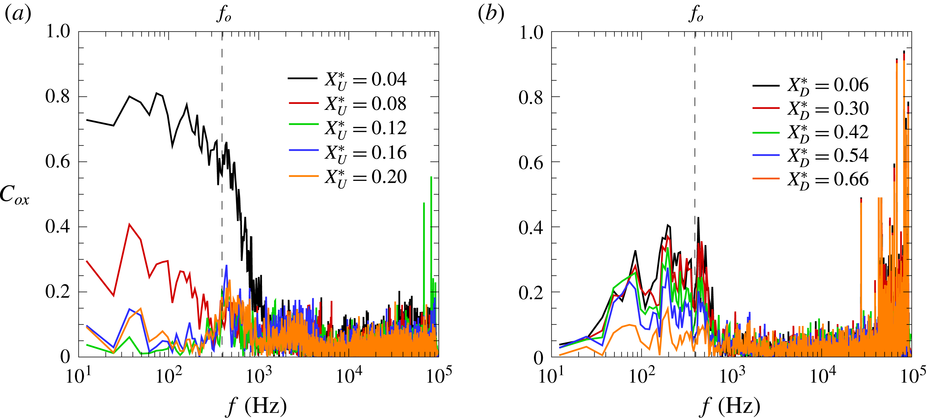
Figure 11. Pressure coherence with reference to
 $X_{U}^{\ast }=0$
: (a) along separation
$X_{U}^{\ast }=0$
: (a) along separation
 $0<X_{U}^{\ast }<0.20$
and (b) close behind the step
$0<X_{U}^{\ast }<0.20$
and (b) close behind the step
 $0.06<X_{D}^{\ast }<0.66$
. Vertical dashed lines mark dominant frequency of 391 Hz at
$0.06<X_{D}^{\ast }<0.66$
. Vertical dashed lines mark dominant frequency of 391 Hz at
 $X_{U}^{\ast }=0$
.
$X_{U}^{\ast }=0$
.
The coherence function
 $C_{ox}$
downstream of separation and with respect to
$C_{ox}$
downstream of separation and with respect to
 $X_{U}^{\ast }=0$
is presented in figure 11(a). At the most downstream extreme of the intermittency length, found at about
$X_{U}^{\ast }=0$
is presented in figure 11(a). At the most downstream extreme of the intermittency length, found at about
 ${\sim}0.75L_{i,U}$
downstream of the mean separation location (
${\sim}0.75L_{i,U}$
downstream of the mean separation location (
 $\unicode[STIX]{x0394}X_{U}^{\ast }\approx 0.12$
), the influence of broadband low-frequency fluctuations is shown to be rapidly reduced. As the flow approaches the plateau region, a signal coherence of
$\unicode[STIX]{x0394}X_{U}^{\ast }\approx 0.12$
), the influence of broadband low-frequency fluctuations is shown to be rapidly reduced. As the flow approaches the plateau region, a signal coherence of
 $C_{ox}\approx 0.4$
starts to be centred at the dominant frequency of the upstream separation (vertical dashed line in the figure). This suggests coherent motions are significant within this region and is interpreted as indicative of the global instability of the bubble at this frequency. Similar analysis on the flow behind the step (figure 11
b) exhibits some level of coherence at the same frequencies yet in a more broadband manner, mostly as a result of the downstream separation region being inherently exposed to a more complex environment, strongly influenced by the upstream separation effects.
$C_{ox}\approx 0.4$
starts to be centred at the dominant frequency of the upstream separation (vertical dashed line in the figure). This suggests coherent motions are significant within this region and is interpreted as indicative of the global instability of the bubble at this frequency. Similar analysis on the flow behind the step (figure 11
b) exhibits some level of coherence at the same frequencies yet in a more broadband manner, mostly as a result of the downstream separation region being inherently exposed to a more complex environment, strongly influenced by the upstream separation effects.
The corresponding
 $fG_{xx}$
contour map in figure 12(a) offers further insight into the overall streamwise evolution of premultiplied spectral content in the
$fG_{xx}$
contour map in figure 12(a) offers further insight into the overall streamwise evolution of premultiplied spectral content in the
 $(f,x)$
-plane, again with reference to the regions a–f highlighted in figure 7(c). Besides the marked low-frequency unsteadiness at separation
$(f,x)$
-plane, again with reference to the regions a–f highlighted in figure 7(c). Besides the marked low-frequency unsteadiness at separation
 $X_{U}^{\ast }=0$
(region a) and reattachment
$X_{U}^{\ast }=0$
(region a) and reattachment
 $X_{D}^{\ast }=1$
(region e), the contour exhibits a well defined and gradual spreading rate of the dominant instabilities associated with the upstream separated shear layers and their convection along the interaction region. The intermittency lengths of the upstream separation
$X_{D}^{\ast }=1$
(region e), the contour exhibits a well defined and gradual spreading rate of the dominant instabilities associated with the upstream separated shear layers and their convection along the interaction region. The intermittency lengths of the upstream separation
 $S_{1}$
and downstream reattachment
$S_{1}$
and downstream reattachment
 $R_{2}$
shocks are respectively
$R_{2}$
shocks are respectively
 $L_{i,U}=18$
mm (
$L_{i,U}=18$
mm (
 $\unicode[STIX]{x0394}X_{U}^{\ast }=0.16$
) and
$\unicode[STIX]{x0394}X_{U}^{\ast }=0.16$
) and
 $L_{i,D}=31.5$
mm (
$L_{i,D}=31.5$
mm (
 $\unicode[STIX]{x0394}X_{D}^{\ast }=0.82$
). The cross-correlations with respect to the signal at separation
$\unicode[STIX]{x0394}X_{D}^{\ast }=0.82$
). The cross-correlations with respect to the signal at separation
 $\unicode[STIX]{x1D70C}_{ox}$
in figure 12(b–d) rely on prior low-pass filtering of the signals at 1 kHz to assess the related low-frequency effects along the interaction, thus removing some of the more complex effects within the downstream separation bubble (note hereafter in the paper no similar filter is applied unless specifically indicated). Results reflect the strong backwards influence of near-wall disturbances within the bubble, where positive delays (
$\unicode[STIX]{x1D70C}_{ox}$
in figure 12(b–d) rely on prior low-pass filtering of the signals at 1 kHz to assess the related low-frequency effects along the interaction, thus removing some of the more complex effects within the downstream separation bubble (note hereafter in the paper no similar filter is applied unless specifically indicated). Results reflect the strong backwards influence of near-wall disturbances within the bubble, where positive delays (
 $\unicode[STIX]{x0394}\unicode[STIX]{x1D70F}>0$
) indicate a later response of the signal at
$\unicode[STIX]{x0394}\unicode[STIX]{x1D70F}>0$
) indicate a later response of the signal at
 $X_{U}^{\ast }=0$
(
$X_{U}^{\ast }=0$
(
 $\unicode[STIX]{x1D70C}_{ox}>0$
). The opposite effect is found just ahead of the step
$\unicode[STIX]{x1D70C}_{ox}>0$
). The opposite effect is found just ahead of the step
 $X_{U}^{\ast }=0.98$
, where the negative correlation and short time delay (
$X_{U}^{\ast }=0.98$
, where the negative correlation and short time delay (
 $\unicode[STIX]{x1D70C}_{ox}<0$
,
$\unicode[STIX]{x1D70C}_{ox}<0$
,
 $\unicode[STIX]{x0394}\unicode[STIX]{x1D70F}<0$
) indicate that pressure rises downstream of the detached shock are generally preceded by a downstream shift of the upstream separation shock, i.e. as pressure at
$\unicode[STIX]{x0394}\unicode[STIX]{x1D70F}<0$
) indicate that pressure rises downstream of the detached shock are generally preceded by a downstream shift of the upstream separation shock, i.e. as pressure at
 $X_{U}^{\ast }=0$
decreases (this is further discussed in § 4). Effectively, this implies that downstream displacements of the separation shock (taken as positive
$X_{U}^{\ast }=0$
decreases (this is further discussed in § 4). Effectively, this implies that downstream displacements of the separation shock (taken as positive
 $\unicode[STIX]{x0394}x$
from
$\unicode[STIX]{x0394}x$
from
 $X_{U}^{\ast }=0$
) are practically in phase with pressure fluctuations near reattachment. Evidence of negative lag times between separation (shock foot) and inside the separation bubble, as well as out of phase correlations between the pressure at separation and reattachment, has been noted in a number of further studies but without a clear mechanism having been established (Babinsky & Harvey Reference Babinsky and Harvey2011). As also found in recent LES studies by Agostini, Larchevêque & Dupont (Reference Agostini, Larchevêque and Dupont2015), the dynamics within the plateau region is relatively more complex, exhibiting varying levels of correlation between shock motions and wall pressure, and with in-phase/anti-phase switches. Further downstream in our case, behind the step, a shrinking of the upstream bubble is found to lead to a subsequent expansion of the local recirculation, as the downstream reattachment shock moves farther from the step inducing a drop in pressure near reattachment
$X_{U}^{\ast }=0$
) are practically in phase with pressure fluctuations near reattachment. Evidence of negative lag times between separation (shock foot) and inside the separation bubble, as well as out of phase correlations between the pressure at separation and reattachment, has been noted in a number of further studies but without a clear mechanism having been established (Babinsky & Harvey Reference Babinsky and Harvey2011). As also found in recent LES studies by Agostini, Larchevêque & Dupont (Reference Agostini, Larchevêque and Dupont2015), the dynamics within the plateau region is relatively more complex, exhibiting varying levels of correlation between shock motions and wall pressure, and with in-phase/anti-phase switches. Further downstream in our case, behind the step, a shrinking of the upstream bubble is found to lead to a subsequent expansion of the local recirculation, as the downstream reattachment shock moves farther from the step inducing a drop in pressure near reattachment
 $R_{2}$
(
$R_{2}$
(
 $\unicode[STIX]{x1D70C}_{ox}>0$
,
$\unicode[STIX]{x1D70C}_{ox}>0$
,
 $\unicode[STIX]{x0394}\unicode[STIX]{x1D70F}<0$
).
$\unicode[STIX]{x0394}\unicode[STIX]{x1D70F}<0$
).

Figure 12. Unsteadiness of highly separated STBLI: (a) pressure power spectral density contour in the
 $(f,x)$
-plane, and correlation with respect to pressure at separation
$(f,x)$
-plane, and correlation with respect to pressure at separation
 $X_{U}^{\ast }=0$
along: (b) upstream separation region, (c) ahead of step and (d) downstream of step. Labels a–f as per figures 7(c) and 10. All measurements at
$X_{U}^{\ast }=0$
along: (b) upstream separation region, (c) ahead of step and (d) downstream of step. Labels a–f as per figures 7(c) and 10. All measurements at
 $\unicode[STIX]{x1D711}^{\ast }=0$
(reference centreline). Cross-correlations apply signal low-pass filtering at 1 kHz to assess low-frequency effects (note no pre-filtering is applied in the remaining results unless specifically indicated). Dashed lines mark distinct contour levels and solid lines are extrapolated fit to the higher levels associated with the upstream shear layer.
$\unicode[STIX]{x1D711}^{\ast }=0$
(reference centreline). Cross-correlations apply signal low-pass filtering at 1 kHz to assess low-frequency effects (note no pre-filtering is applied in the remaining results unless specifically indicated). Dashed lines mark distinct contour levels and solid lines are extrapolated fit to the higher levels associated with the upstream shear layer.

Figure 13. Point to point pressure coherence along upstream separation region: (a) over
 $0.16\leqslant X_{U}^{\ast }\leqslant 0.55$
and (b)
$0.16\leqslant X_{U}^{\ast }\leqslant 0.55$
and (b)
 $0.55\leqslant X_{U}^{\ast }\leqslant 0.90$
. Respectively with reference to previous signal at
$0.55\leqslant X_{U}^{\ast }\leqslant 0.90$
. Respectively with reference to previous signal at
 $\unicode[STIX]{x0394}X_{U}^{\ast }=-0.04$
for each location. Zoomed into
$\unicode[STIX]{x0394}X_{U}^{\ast }=-0.04$
for each location. Zoomed into
 $10^{2}$
–
$10^{2}$
–
 $10^{5}$
Hz range to highlight shear layer effects.
$10^{5}$
Hz range to highlight shear layer effects.

Figure 14. Point to point phase velocity along upstream separation region normalised with local spectrum as
 $v_{\unicode[STIX]{x1D719}}G_{xx}/G_{f,max}$
: (a) over
$v_{\unicode[STIX]{x1D719}}G_{xx}/G_{f,max}$
: (a) over
 $0.16\leqslant X_{U}^{\ast }\leqslant 0.55$
and (b)
$0.16\leqslant X_{U}^{\ast }\leqslant 0.55$
and (b)
 $0.55\leqslant X_{U}^{\ast }\leqslant 0.90$
. Locations and respective legends as per figure 13 above. Zoomed into
$0.55\leqslant X_{U}^{\ast }\leqslant 0.90$
. Locations and respective legends as per figure 13 above. Zoomed into
 $10^{2}$
–
$10^{2}$
–
 $10^{5}$
Hz range as per figure 13.
$10^{5}$
Hz range as per figure 13.

Figure 15. Pressure correlation in the azimuthal direction: (a) at
 $X_{U}^{\ast }=0$
, (b)
$X_{U}^{\ast }=0$
, (b)
 $X_{U}^{\ast }=0.20$
and (c)
$X_{U}^{\ast }=0.20$
and (c)
 $X_{U}^{\ast }=0.98$
. Between
$X_{U}^{\ast }=0.98$
. Between
 $0\leqslant \unicode[STIX]{x1D711}^{\ast }\leqslant 0.283$
(up to
$0\leqslant \unicode[STIX]{x1D711}^{\ast }\leqslant 0.283$
(up to
 $\unicode[STIX]{x1D711}=32.5$
mm from centreline), with reference to
$\unicode[STIX]{x1D711}=32.5$
mm from centreline), with reference to
 $\unicode[STIX]{x1D711}^{\ast }=0$
. Cross-correlations apply signal bandpass filtering at 1 kHz to assess low-frequency effects.
$\unicode[STIX]{x1D711}^{\ast }=0$
. Cross-correlations apply signal bandpass filtering at 1 kHz to assess low-frequency effects.
As shown in figure 13, the point to point coherence
 $C_{x-1,x}$
along the recirculation region (taken in
$C_{x-1,x}$
along the recirculation region (taken in
 $X_{U}^{\ast }=0.04$
steps) is relatively high with a slight increase from
$X_{U}^{\ast }=0.04$
steps) is relatively high with a slight increase from
 $C_{x-1,x}=0.4$
to 0.7 down to
$C_{x-1,x}=0.4$
to 0.7 down to
 $X_{U}^{\ast }=0.35$
and centred at the shear layer frequencies (note comparison with the spectra in figure 10 finds the same maxima coinciding with the high coherence region). The coherence is subsequently maintained at
$X_{U}^{\ast }=0.35$
and centred at the shear layer frequencies (note comparison with the spectra in figure 10 finds the same maxima coinciding with the high coherence region). The coherence is subsequently maintained at
 $C_{x-1,x}\approx 0.7$
, with the associated dominant frequency following the earlier noted shift with lower frequencies as found for shear layer instabilities. Relatively high and broadband coherence is found for frequencies below
$C_{x-1,x}\approx 0.7$
, with the associated dominant frequency following the earlier noted shift with lower frequencies as found for shear layer instabilities. Relatively high and broadband coherence is found for frequencies below
 $10^{3}$
Hz along the recirculation region (except just ahead of the step). The trends thus clearly evidence the formation of shear layer eddies and are for instance consistent with those in the subsonic experimental studies by Na & Moin (Reference Na and Moin1998), on a highly separated (
$10^{3}$
Hz along the recirculation region (except just ahead of the step). The trends thus clearly evidence the formation of shear layer eddies and are for instance consistent with those in the subsonic experimental studies by Na & Moin (Reference Na and Moin1998), on a highly separated (
 ${\sim}20\unicode[STIX]{x1D6FF}_{o}$
) turbulent boundary layer, where large-scale turbulent structures in the shear layer were found to grow in size and coherence as they convected along the separation. In the DNS by Chong et al. (Reference Chong, Soria, Perry, Chacin and Na1998), on an incompressible separation of length
${\sim}20\unicode[STIX]{x1D6FF}_{o}$
) turbulent boundary layer, where large-scale turbulent structures in the shear layer were found to grow in size and coherence as they convected along the separation. In the DNS by Chong et al. (Reference Chong, Soria, Perry, Chacin and Na1998), on an incompressible separation of length
 ${\sim}5\unicode[STIX]{x1D6FF}_{o}$
, the high vorticity within the shear layer could be further tracked to originate near the near-wall region (near separation), roughly within the momentum thickness
${\sim}5\unicode[STIX]{x1D6FF}_{o}$
, the high vorticity within the shear layer could be further tracked to originate near the near-wall region (near separation), roughly within the momentum thickness
 $\unicode[STIX]{x1D703}_{o}$
and with coherent structures eventually diffusing closer to reattachment.
$\unicode[STIX]{x1D703}_{o}$
and with coherent structures eventually diffusing closer to reattachment.
In figure 14, the phase velocity at different stages of shear layer development is presented scaled by the normalised local frequency spectra
 $v_{\unicode[STIX]{x1D719}}G_{xx}/G_{f,max}$
, where
$v_{\unicode[STIX]{x1D719}}G_{xx}/G_{f,max}$
, where
 $v_{\unicode[STIX]{x1D719}}=2\unicode[STIX]{x03C0}f\unicode[STIX]{x1D709}/\unicode[STIX]{x1D719}$
and
$v_{\unicode[STIX]{x1D719}}=2\unicode[STIX]{x03C0}f\unicode[STIX]{x1D709}/\unicode[STIX]{x1D719}$
and
 $\unicode[STIX]{x1D719}$
is the phase deduced from the cross-spectra between adjacent sensor locations (note the rather unconventional
$\unicode[STIX]{x1D719}$
is the phase deduced from the cross-spectra between adjacent sensor locations (note the rather unconventional
 $G_{xx}/G_{f,max}$
scaling is here used as an effective filter to extract the phase velocity associated with the local characteristic frequency of the shear layer;
$G_{xx}/G_{f,max}$
scaling is here used as an effective filter to extract the phase velocity associated with the local characteristic frequency of the shear layer;
 $v_{\unicode[STIX]{x1D719}}$
alone remains generally at a flat level within the shear layer range). As the shear layer develops and shifts to lower frequencies over the plateau region (
$v_{\unicode[STIX]{x1D719}}$
alone remains generally at a flat level within the shear layer range). As the shear layer develops and shifts to lower frequencies over the plateau region (
 $X_{U}^{\ast }\geqslant 0.2$
), its convection exhibits a moderate deceleration. Upon inception of the shear layer at approximately
$X_{U}^{\ast }\geqslant 0.2$
), its convection exhibits a moderate deceleration. Upon inception of the shear layer at approximately
 $X_{U}^{\ast }=0.20$
(more precisely between
$X_{U}^{\ast }=0.20$
(more precisely between
 $X_{U}^{\ast }=0.16$
and 0.20, noting the incipient enhancement at high frequencies for the former in figure 10
a), a phase velocity of
$X_{U}^{\ast }=0.16$
and 0.20, noting the incipient enhancement at high frequencies for the former in figure 10
a), a phase velocity of
 $v_{\unicode[STIX]{x1D719}}=364~\text{m}~\text{s}^{-1}$
(
$v_{\unicode[STIX]{x1D719}}=364~\text{m}~\text{s}^{-1}$
(
 $\pm 8\,\%$
) is noticed at the local dominant frequency. This then decreases gradually down to
$\pm 8\,\%$
) is noticed at the local dominant frequency. This then decreases gradually down to
 ${\sim}296~\text{m}~\text{s}^{-1}$
at
${\sim}296~\text{m}~\text{s}^{-1}$
at
 $X_{U}^{\ast }=0.86$
, slightly ahead of the detached shock – while the dominant frequency decreases from 37.5 kHz at a significantly faster rate (a drop of approximately a factor 4 between these two locations, as per the spectra in figure 10). Immediately ahead of the step, the shear layer is eventually disrupted and the local phase velocity is no longer representative of the – until this point – predominant shear layer influence, but instead appears dominated by higher velocity perturbations (more details on the localised compression–expansion effects near the step are given in the following section).
$X_{U}^{\ast }=0.86$
, slightly ahead of the detached shock – while the dominant frequency decreases from 37.5 kHz at a significantly faster rate (a drop of approximately a factor 4 between these two locations, as per the spectra in figure 10). Immediately ahead of the step, the shear layer is eventually disrupted and the local phase velocity is no longer representative of the – until this point – predominant shear layer influence, but instead appears dominated by higher velocity perturbations (more details on the localised compression–expansion effects near the step are given in the following section).
As shown in figure 15(a), the cross-correlation of the signals obtained in the azimuthal direction
 $\unicode[STIX]{x1D70C}_{o,\unicode[STIX]{x1D719}}$
and with reference to local pressure at centreline
$\unicode[STIX]{x1D70C}_{o,\unicode[STIX]{x1D719}}$
and with reference to local pressure at centreline
 $\unicode[STIX]{x1D711}^{\ast }=0$
(
$\unicode[STIX]{x1D711}^{\ast }=0$
(
 $\unicode[STIX]{x1D711}^{\ast }=\unicode[STIX]{x1D711}/L_{U}$
) further reveal the influence of large-scale spanwise effects at
$\unicode[STIX]{x1D711}^{\ast }=\unicode[STIX]{x1D711}/L_{U}$
) further reveal the influence of large-scale spanwise effects at
 $X_{U}^{\ast }=0$
and
$X_{U}^{\ast }=0$
and
 $X_{U}^{\ast }=0.2$
(figure 15
a–b) eventually reaching a reversal in the correlation sign by
$X_{U}^{\ast }=0.2$
(figure 15
a–b) eventually reaching a reversal in the correlation sign by
 $X_{U}^{\ast }=0.98$
, behind the bow shock (figure 15
c). While effects associated with potential spanwise instabilities are uncertain, partly due to the experimental limitations to cover the complete perimeter, similar signs of a lateral influence have been observed in other studies – e.g. in DNS by Priebe & Martin (Reference Priebe and Martin2012), where a transverse flapping of the interaction was documented for a flat plate STBLI over a
$X_{U}^{\ast }=0.98$
, behind the bow shock (figure 15
c). While effects associated with potential spanwise instabilities are uncertain, partly due to the experimental limitations to cover the complete perimeter, similar signs of a lateral influence have been observed in other studies – e.g. in DNS by Priebe & Martin (Reference Priebe and Martin2012), where a transverse flapping of the interaction was documented for a flat plate STBLI over a
 $24^{\circ }$
-ramp at Mach 2.9. As shown in the supplementary high-speed schlieren movies (clips available online at https://doi.org/10.1017/jfm.2017.522), the separation shock unsteadiness on two opposite sides of the model (
$24^{\circ }$
-ramp at Mach 2.9. As shown in the supplementary high-speed schlieren movies (clips available online at https://doi.org/10.1017/jfm.2017.522), the separation shock unsteadiness on two opposite sides of the model (
 $\unicode[STIX]{x1D711}=0^{\circ }$
and
$\unicode[STIX]{x1D711}=0^{\circ }$
and
 $180^{\circ }$
) is in poor cross-correlation thus suggesting spanwise instabilities at this more upstream location are relatively weaker and within about
$180^{\circ }$
) is in poor cross-correlation thus suggesting spanwise instabilities at this more upstream location are relatively weaker and within about
 $\pm 0.2\unicode[STIX]{x0394}\unicode[STIX]{x1D711}^{\ast }$
as per figure 15(a). The lateral instability effects associated with the interaction are however highly complex and beyond the scope of the present study.
$\pm 0.2\unicode[STIX]{x0394}\unicode[STIX]{x1D711}^{\ast }$
as per figure 15(a). The lateral instability effects associated with the interaction are however highly complex and beyond the scope of the present study.

Figure 16. Measurements over front face of the step: (a) mean pressure and flow schematic, (b) power spectral density (normalised by maximum of the spectrum at
 $X_{U}^{\ast }=0.98$
), (c) time correlation with pressure signal at
$X_{U}^{\ast }=0.98$
), (c) time correlation with pressure signal at
 $X_{U}^{\ast }=0$
and (d) coherence with respect to pressure signal at
$X_{U}^{\ast }=0$
and (d) coherence with respect to pressure signal at
 $X_{U}^{\ast }=0$
. Locations over step front normalised as
$X_{U}^{\ast }=0$
. Locations over step front normalised as
 $Y_{F}^{\ast }=y/h$
, where
$Y_{F}^{\ast }=y/h$
, where
 $y$
is wall-normal distance with respect to base cylinder body. Vertical dashed line in panel (
$y$
is wall-normal distance with respect to base cylinder body. Vertical dashed line in panel (
 $a$
) marks mean pressure location at
$a$
) marks mean pressure location at
 $X_{U}^{\ast }=0.98$
(over base cylinder) and schematic indicates sensor arrangement. In panel (
$X_{U}^{\ast }=0.98$
(over base cylinder) and schematic indicates sensor arrangement. In panel (
 $d$
), it marks the dominant frequency of 391 Hz at
$d$
), it marks the dominant frequency of 391 Hz at
 $X_{U}^{\ast }=0$
. The legend is common to panels (
$X_{U}^{\ast }=0$
. The legend is common to panels (
 $b-d$
).
$b-d$
).

Figure 17. Measurements over top surface of the step: (a) mean pressure and flow schematic, (b) power spectral density (normalised by maximum of the spectrum at
 $X_{U}^{\ast }=0.98$
), (c) time correlation with pressure signal at
$X_{U}^{\ast }=0.98$
), (c) time correlation with pressure signal at
 $X_{U}^{\ast }=0$
and (d) coherence with respect to pressure signal at
$X_{U}^{\ast }=0$
and (d) coherence with respect to pressure signal at
 $X_{U}^{\ast }=0$
. Locations over step upper surface normalised as
$X_{U}^{\ast }=0$
. Locations over step upper surface normalised as
 $X_{T}^{\ast }=x/l_{S}$
, where
$X_{T}^{\ast }=x/l_{S}$
, where
 $X_{T}^{\ast }=0$
corresponds to step leading edge and
$X_{T}^{\ast }=0$
corresponds to step leading edge and
 $X_{T}^{\ast }=1$
to step trailing edge (note also that step length to height ratio is kept at
$X_{T}^{\ast }=1$
to step trailing edge (note also that step length to height ratio is kept at
 $l_{S}/h=1$
throughout the paper except for the additional cases in figure 19
a–b). Horizontal dashed line in panel (
$l_{S}/h=1$
throughout the paper except for the additional cases in figure 19
a–b). Horizontal dashed line in panel (
 $a$
) marks mean reference wall pressure
$a$
) marks mean reference wall pressure
 $p_{u}$
(undisturbed at
$p_{u}$
(undisturbed at
 $X_{U}^{\ast }=0$
) and schematic indicates sensor arrangement. Vertical dashed line in panel (
$X_{U}^{\ast }=0$
) and schematic indicates sensor arrangement. Vertical dashed line in panel (
 $d$
) marks the dominant frequency of 391 Hz at
$d$
) marks the dominant frequency of 391 Hz at
 $X_{U}^{\ast }=0$
. Legend above is common to panels (
$X_{U}^{\ast }=0$
. Legend above is common to panels (
 $b{-}d$
).
$b{-}d$
).
3.4 Flow over step front and upper surfaces
Following the above, the mechanisms associated with the flow along and in close vicinity of the step were analysed. The mean pressure over the front face can be found in figure 16(a) together with a schematic of the instrumentation arrangement (with five sensors placed within the step and spaced at
 $\unicode[STIX]{x0394}y/\unicode[STIX]{x1D6FF}_{o}=1$
starting from the wall). Results show a first decrease in pressure from the 34.7 kPa near the corner
$\unicode[STIX]{x0394}y/\unicode[STIX]{x1D6FF}_{o}=1$
starting from the wall). Results show a first decrease in pressure from the 34.7 kPa near the corner
 $Y_{F}^{\ast }=0.17$
(similar to the levels at
$Y_{F}^{\ast }=0.17$
(similar to the levels at
 $X_{U}^{\ast }=0.98$
) and down to 29.3 kPa at approximately half the step height
$X_{U}^{\ast }=0.98$
) and down to 29.3 kPa at approximately half the step height
 $Y_{F}^{\ast }=0.51$
, where
$Y_{F}^{\ast }=0.51$
, where
 $Y_{F}^{\ast }=y/h$
. This is then followed by a further overshoot up to 44.3 kPa at
$Y_{F}^{\ast }=y/h$
. This is then followed by a further overshoot up to 44.3 kPa at
 $Y_{F}^{\ast }=0.84$
, thus showing that the highest pressures over the front surface take place near the upper edge of the step (the bow shock is better defined near this location). The spectra in figure 16(b) find that the dominant frequency near the base cylinder at
$Y_{F}^{\ast }=0.84$
, thus showing that the highest pressures over the front surface take place near the upper edge of the step (the bow shock is better defined near this location). The spectra in figure 16(b) find that the dominant frequency near the base cylinder at
 $Y_{F}^{\ast }=0.17$
is 8.45 kHz and hence similar to that measured at
$Y_{F}^{\ast }=0.17$
is 8.45 kHz and hence similar to that measured at
 $X_{U}^{\ast }=0.98$
(figure 10
c). A second and higher-frequency dominant mode is found to arise at 20.1 kHz by
$X_{U}^{\ast }=0.98$
(figure 10
c). A second and higher-frequency dominant mode is found to arise at 20.1 kHz by
 $Y_{F}^{\ast }=0.34$
, both instabilities being significant in this region. The latter then gains strength at locations closer to the upper edge,
$Y_{F}^{\ast }=0.34$
, both instabilities being significant in this region. The latter then gains strength at locations closer to the upper edge,
 $Y_{F}^{\ast }=0.68$
and
$Y_{F}^{\ast }=0.68$
and
 $Y_{F}^{\ast }=0.84$
(the earlier near-wall instability having vanished) and with a shift to lower frequencies in a similar fashion to that found along the upstream separation – thus being likely associated with a shear layer within what appears to comply to a secondary (counter-rotating) recirculation near the front face of the step. An increase in low-frequency energy (
$Y_{F}^{\ast }=0.84$
(the earlier near-wall instability having vanished) and with a shift to lower frequencies in a similar fashion to that found along the upstream separation – thus being likely associated with a shear layer within what appears to comply to a secondary (counter-rotating) recirculation near the front face of the step. An increase in low-frequency energy (
 ${<}10^{3}$
Hz) is only perceived closer to the upper edge, well within the primary recirculation (e.g. as sketched in figure 1
a). As further found in the cross-correlation plot in figure 16(c), the pressure at different locations over the front surface of the step is in negative correlation (
${<}10^{3}$
Hz) is only perceived closer to the upper edge, well within the primary recirculation (e.g. as sketched in figure 1
a). As further found in the cross-correlation plot in figure 16(c), the pressure at different locations over the front surface of the step is in negative correlation (
 $\unicode[STIX]{x1D70C}_{oy}\approx -0.25$
) with that at
$\unicode[STIX]{x1D70C}_{oy}\approx -0.25$
) with that at
 $X_{U}^{\ast }=0$
; that is, an upstream shift of the separation shock (hence local pressure decrease at
$X_{U}^{\ast }=0$
; that is, an upstream shift of the separation shock (hence local pressure decrease at
 $S_{1}$
) is often quickly followed by an increase in pressure behind the step and vice versa. As found in figure 16(d), there is practically negligible coherence with respect to the pressure at separation
$S_{1}$
) is often quickly followed by an increase in pressure behind the step and vice versa. As found in figure 16(d), there is practically negligible coherence with respect to the pressure at separation
 $X_{U}^{\ast }=0$
, with only approximately
$X_{U}^{\ast }=0$
, with only approximately
 $C_{oy}\approx 0.2$
at the lower frequencies, particularly so near the dominant low-frequency instability of 391 Hz – this being more broadband within the secondary recirculation (cf.
$C_{oy}\approx 0.2$
at the lower frequencies, particularly so near the dominant low-frequency instability of 391 Hz – this being more broadband within the secondary recirculation (cf.
 $S_{1}$
spectra in figure 10
a).
$S_{1}$
spectra in figure 10
a).
The respective results over the upper surface of the step can be found in figure 17, with the pertinent sensor arrangement indicated in the figure as well. Following a localised expansion near the leading edge, the mean pressure is seen to have dropped drastically from the 35.8 kPa ahead of the step down to 14.6 kPa (
 ${\sim}1.5p_{u}$
) by
${\sim}1.5p_{u}$
) by
 $X_{T}^{\ast }=0.16$
, where
$X_{T}^{\ast }=0.16$
, where
 $X_{T}^{\ast }=x/l_{s}$
. This then continues to expand slightly down to 12.7 kPa by
$X_{T}^{\ast }=x/l_{s}$
. This then continues to expand slightly down to 12.7 kPa by
 $X_{T}^{\ast }=0.87$
. At the same time, the dominant frequency (figure 17
b) is found to shift from approximately 6 to 3 kHz between
$X_{T}^{\ast }=0.87$
. At the same time, the dominant frequency (figure 17
b) is found to shift from approximately 6 to 3 kHz between
 $X_{T}^{\ast }=0.16$
and 0.51, to then recover to higher frequencies (15 kHz at
$X_{T}^{\ast }=0.16$
and 0.51, to then recover to higher frequencies (15 kHz at
 $X_{T}^{\ast }=0.87$
) closer to step trailing edge. Similarly to the effects found over the front face, the pressure along the upper surface is also in negative correlation with that at separation (figure 17
c). The coherence with respect to separation is again fairly low, with also up to a
$X_{T}^{\ast }=0.87$
) closer to step trailing edge. Similarly to the effects found over the front face, the pressure along the upper surface is also in negative correlation with that at separation (figure 17
c). The coherence with respect to separation is again fairly low, with also up to a
 $C_{ox}\approx 0.2$
centred at the characteristic low-frequency instability of the bubble (figure 17
d). The flow near reattachment is therefore of high complexity and involves the co-existence of a localised stagnation near the upper section in the front face of the step and a sudden expansion over the edge.
$C_{ox}\approx 0.2$
centred at the characteristic low-frequency instability of the bubble (figure 17
d). The flow near reattachment is therefore of high complexity and involves the co-existence of a localised stagnation near the upper section in the front face of the step and a sudden expansion over the edge.
Results overall evidence that the frequency associated with bubble pulsations – best isolated in the separation frequency spectra at
 $X_{U}^{\ast }=0$
(figure 10
a) – effectively acts as a global mode imposed across the interaction and strongly influences the downstream flow behind the step. In co-existence with this effect, the flow dynamics along the separation is strongly dominated by the formation of a shear layer bounded by the low-speed flow inside the separation and the outer high-speed flow (behind the separation shock) and characterised by its high-to-moderate frequencies,
$X_{U}^{\ast }=0$
(figure 10
a) – effectively acts as a global mode imposed across the interaction and strongly influences the downstream flow behind the step. In co-existence with this effect, the flow dynamics along the separation is strongly dominated by the formation of a shear layer bounded by the low-speed flow inside the separation and the outer high-speed flow (behind the separation shock) and characterised by its high-to-moderate frequencies,
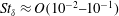 $St_{\unicode[STIX]{x1D6FF}}\approx O(10^{-2}{-}10^{-1})$
. To shed further light into the role of the shear layer on interaction unsteadiness, a detailed assessment on the related spectral quantities over the recirculation region is presented next.
$St_{\unicode[STIX]{x1D6FF}}\approx O(10^{-2}{-}10^{-1})$
. To shed further light into the role of the shear layer on interaction unsteadiness, a detailed assessment on the related spectral quantities over the recirculation region is presented next.
4 Upstream separation shear layer
4.1 Shear layer evolution
The results so far have demonstrated the strong predominance of the upstream shear layer effect within the recirculation region and its interference on the downstream separation behind the step. As such, the analysis hereafter in the paper focuses on the unsteady effects within the upstream separation region only. The streamwise evolution of the characteristic frequency
 $f_{ch}$
along the interaction is summed up in figure 18(a), overlapped with the mean pressure for reference, and where
$f_{ch}$
along the interaction is summed up in figure 18(a), overlapped with the mean pressure for reference, and where
 $f_{ch}$
is directly extracted from the maxima of the spectra at each sensor location (from figure 10) with an estimated uncertainty of 2 %. Following the low dominant frequencies near the location of upstream separation
$f_{ch}$
is directly extracted from the maxima of the spectra at each sensor location (from figure 10) with an estimated uncertainty of 2 %. Following the low dominant frequencies near the location of upstream separation
 $S_{1}$
(
$S_{1}$
(
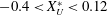 $-0.4<X_{U}^{\ast }<0.12$
),
$-0.4<X_{U}^{\ast }<0.12$
),
 $f_{ch}$
is found to increase rapidly and to reach its peak upon shear layer inception by approximately
$f_{ch}$
is found to increase rapidly and to reach its peak upon shear layer inception by approximately
 $X_{U}^{\ast }=0.20$
(
$X_{U}^{\ast }=0.20$
(
 $f_{i}=37.5$
kHz), to then drop monotonically along the recirculation region (note the origin of the left axis in the figure is set to match the
$f_{i}=37.5$
kHz), to then drop monotonically along the recirculation region (note the origin of the left axis in the figure is set to match the
 $p_{u}$
levels in the incoming interaction for comparison). The gradual reduction in
$p_{u}$
levels in the incoming interaction for comparison). The gradual reduction in
 $f_{ch}$
eventually attains a level of 8.8 kHz prior to reattachment over the top edge of the step, with a further drop and subsequent recovery as a result of the localised effects over the top surface (as earlier shown in figure 10,
$f_{ch}$
eventually attains a level of 8.8 kHz prior to reattachment over the top edge of the step, with a further drop and subsequent recovery as a result of the localised effects over the top surface (as earlier shown in figure 10,
 $f_{ch}$
then remains approximately at
$f_{ch}$
then remains approximately at
 ${\sim}12$
kHz within the relaxation region, except near reattachment
${\sim}12$
kHz within the relaxation region, except near reattachment
 $R_{2}$
, where
$R_{2}$
, where
 $f_{ch}=3.55$
kHz). The schlieren captures in clear detail the formation of the shear layer and associated acoustic waves emanating from shear layer eddies. The three samples in figure 18(b) further suggest the earlier noted irregularities are in great part related to the evolution of these disturbances. These samples are selected to capture the instants where the separation bubble is about to start collapsing (separation
$f_{ch}=3.55$
kHz). The schlieren captures in clear detail the formation of the shear layer and associated acoustic waves emanating from shear layer eddies. The three samples in figure 18(b) further suggest the earlier noted irregularities are in great part related to the evolution of these disturbances. These samples are selected to capture the instants where the separation bubble is about to start collapsing (separation
 $x_{S}$
at the most upstream extreme of intermittency length
$x_{S}$
at the most upstream extreme of intermittency length
 $x_{i,1}=x_{o}-4.5$
mm), when it is at the mean separation location
$x_{i,1}=x_{o}-4.5$
mm), when it is at the mean separation location
 $x_{o}$
(
$x_{o}$
(
 $X_{U}^{\ast }=0$
) and where it is about to start recovering (separation at the most downstream extreme of intermittency length
$X_{U}^{\ast }=0$
) and where it is about to start recovering (separation at the most downstream extreme of intermittency length
 $x_{i,2}=x_{o}+13.5$
mm, closest to the step). It is worth noting that by ‘intermittency length’ we are not strictly referring to shock foot oscillations but rather to the region of dominant low-frequency unsteadiness in wall pressure, with fluctuations oscillating above the undisturbed levels at the most downstream locations, e.g. as per the pressure traces in figure 7(a).
$x_{i,2}=x_{o}+13.5$
mm, closest to the step). It is worth noting that by ‘intermittency length’ we are not strictly referring to shock foot oscillations but rather to the region of dominant low-frequency unsteadiness in wall pressure, with fluctuations oscillating above the undisturbed levels at the most downstream locations, e.g. as per the pressure traces in figure 7(a).

Figure 18. Shear layer effect upon separation: (a) streamwise evolution of characteristic frequency
 $f_{ch}$
(black circles, right axis) overlapped with corresponding mean pressure values (grey diamond symbols, left axis) and pressure measurements on opposite side of the model (white diamond symbols, left axis), together with
$f_{ch}$
(black circles, right axis) overlapped with corresponding mean pressure values (grey diamond symbols, left axis) and pressure measurements on opposite side of the model (white diamond symbols, left axis), together with
 $f_{ch}$
over step face (white triangles, right axis) and schlieren image (
$f_{ch}$
over step face (white triangles, right axis) and schlieren image (
 $\unicode[STIX]{x0394}t=12.5~\unicode[STIX]{x03BC}\text{s}$
exposure) shown below; and with (b) sample measurements and schlieren for separation at
$\unicode[STIX]{x0394}t=12.5~\unicode[STIX]{x03BC}\text{s}$
exposure) shown below; and with (b) sample measurements and schlieren for separation at
 $x_{i,1}=x_{o}-4.5$
mm,
$x_{i,1}=x_{o}-4.5$
mm,
 $x_{o}$
and
$x_{o}$
and
 $x_{o}+13.5~\text{mm}$
(symbols as per figure 8), and where
$x_{o}+13.5~\text{mm}$
(symbols as per figure 8), and where
 $x_{i,1}$
and
$x_{i,1}$
and
 $x_{i,2}$
are the most upstream and downstream extremes of the intermittency length (as per the local
$x_{i,2}$
are the most upstream and downstream extremes of the intermittency length (as per the local
 $\unicode[STIX]{x1D70E}_{p}/p$
and PSD in figures 7 and 10). Vertical dashed lines indicates
$\unicode[STIX]{x1D70E}_{p}/p$
and PSD in figures 7 and 10). Vertical dashed lines indicates
 $S_{1}$
location and horizontal line is reference pressure over base cylinder without the step.
$S_{1}$
location and horizontal line is reference pressure over base cylinder without the step.

Figure 19. Shear layer evolution along upstream separation region: (a) dominant frequency
 $f_{ch}$
for step length to height ratios
$f_{ch}$
for step length to height ratios
 $l_{S}/h=1$
(diamond symbols),
$l_{S}/h=1$
(diamond symbols),
 $l_{S}/h=2/3$
(circles) and
$l_{S}/h=2/3$
(circles) and
 $l_{S}/h=1/3$
(squares) and with minimum and maximum frequency within respective ranges of dominant shear layer influence extracted from the main case
$l_{S}/h=1/3$
(squares) and with minimum and maximum frequency within respective ranges of dominant shear layer influence extracted from the main case
 $l_{S}/h=1$
(downwards and upwards triangles) as indicated in the schematic; (b) spectral energy for
$l_{S}/h=1$
(downwards and upwards triangles) as indicated in the schematic; (b) spectral energy for
 $l_{S}/h=1$
case at
$l_{S}/h=1$
case at
 $f<1$
kHz (black diamonds) and
$f<1$
kHz (black diamonds) and
 $f>1$
kHz (grey diamonds), and for
$f>1$
kHz (grey diamonds), and for
 $l_{S}/h=2/3$
(circles) and
$l_{S}/h=2/3$
(circles) and
 $l_{S}/h=1/3$
(squares) cases respectively as grey and white symbols for
$l_{S}/h=1/3$
(squares) cases respectively as grey and white symbols for
 $f<1$
kHz and
$f<1$
kHz and
 $f>1$
kHz; dashed line indicates base shear layer energy just before location of incipient shear layer formation
$f>1$
kHz; dashed line indicates base shear layer energy just before location of incipient shear layer formation
 $X_{U}^{\ast }=0.16$
(energy is normalised with respect to total energy for highest pressure location,
$X_{U}^{\ast }=0.16$
(energy is normalised with respect to total energy for highest pressure location,
 $X_{U}^{\ast }=0.98$
); together with (c) point to point correlation
$X_{U}^{\ast }=0.98$
); together with (c) point to point correlation
 $\unicode[STIX]{x1D70C}_{ox}$
along separation region with reference to
$\unicode[STIX]{x1D70C}_{ox}$
along separation region with reference to
 $X_{U}^{\ast }=0$
(black symbols) and respective time delay (grey symbols) distinguishing accordingly between positive
$X_{U}^{\ast }=0$
(black symbols) and respective time delay (grey symbols) distinguishing accordingly between positive
 $\unicode[STIX]{x1D70F}>0$
(triangle up) and negative
$\unicode[STIX]{x1D70F}>0$
(triangle up) and negative
 $\unicode[STIX]{x1D70F}<0$
delays (triangle down).
$\unicode[STIX]{x1D70F}<0$
delays (triangle down).
In figure 19(a), the dominant frequencies along the upstream separation length are presented to compare the pertinent effects for the interactions induced by two further step cases of the same height (
 $h/\unicode[STIX]{x1D6FF}_{o}=5.9$
) but with a shorter length from step leading to trailing edge, corresponding to
$h/\unicode[STIX]{x1D6FF}_{o}=5.9$
) but with a shorter length from step leading to trailing edge, corresponding to
 $l_{S}/h=2/3$
and
$l_{S}/h=2/3$
and
 $1/3$
. The close overlap among these cases corroborates that the effect of step length bears no influence on the upstream separation for the cases hereby considered (
$1/3$
. The close overlap among these cases corroborates that the effect of step length bears no influence on the upstream separation for the cases hereby considered (
 $l_{S}/h\geqslant 1/3$
) and so the boundary layer may well be deemed to reattach fully over the upper surface. The minimum and maximum frequencies associated with the shear layer are also indicated as a means to inspect the evolution in the skew of its energy distribution, to offer direct comparison with the variation in the given values of
$l_{S}/h\geqslant 1/3$
) and so the boundary layer may well be deemed to reattach fully over the upper surface. The minimum and maximum frequencies associated with the shear layer are also indicated as a means to inspect the evolution in the skew of its energy distribution, to offer direct comparison with the variation in the given values of
 $f_{ch}$
, i.e. at
$f_{ch}$
, i.e. at
 $f_{ch}\pm 3\unicode[STIX]{x1D70E}_{f}$
below and above the dominant frequency associated with the shear layer (refer to the schematic in figure 19
a). The assessment in terms of signal skew and kurtosis was not found to be as useful given the variations in the base broadband and low-frequency energy components. Through comparison with the original spectra in figure 10, the distribution is noted to start negatively skewed, with maxima closer to the highest dominant frequencies, and to then adopt a practically Gaussian distribution by the middle of the interaction
$f_{ch}\pm 3\unicode[STIX]{x1D70E}_{f}$
below and above the dominant frequency associated with the shear layer (refer to the schematic in figure 19
a). The assessment in terms of signal skew and kurtosis was not found to be as useful given the variations in the base broadband and low-frequency energy components. Through comparison with the original spectra in figure 10, the distribution is noted to start negatively skewed, with maxima closer to the highest dominant frequencies, and to then adopt a practically Gaussian distribution by the middle of the interaction
 $X_{U}^{\ast }\approx 0.5$
, with eventually a positive skew near reattachment (believed related to a varying immersion of the shear layer within the recirculation as further discussed in § 4.2). The respective values of normalised standard deviation
$X_{U}^{\ast }\approx 0.5$
, with eventually a positive skew near reattachment (believed related to a varying immersion of the shear layer within the recirculation as further discussed in § 4.2). The respective values of normalised standard deviation
 $\unicode[STIX]{x1D70E}_{p}/p$
, the local Strouhal numbers
$\unicode[STIX]{x1D70E}_{p}/p$
, the local Strouhal numbers
 $St_{L}$
and
$St_{L}$
and
 $St_{\unicode[STIX]{x1D6FF}}$
and other related quantities may be found tabulated in table 2.
$St_{\unicode[STIX]{x1D6FF}}$
and other related quantities may be found tabulated in table 2.
Table 2. Properties along upstream separation: mean pressure
 $p$
, standard deviation
$p$
, standard deviation
 $\unicode[STIX]{x1D70E}_{p}$
, normalised standard deviation
$\unicode[STIX]{x1D70E}_{p}$
, normalised standard deviation
 $\unicode[STIX]{x1D70E}_{p}/p$
, characteristic frequency
$\unicode[STIX]{x1D70E}_{p}/p$
, characteristic frequency
 $f_{ch}$
, Strouhal number based on separation length
$f_{ch}$
, Strouhal number based on separation length
 $St_{L}$
, on boundary layer thickness
$St_{L}$
, on boundary layer thickness
 $St_{\unicode[STIX]{x1D6FF}}$
, energy at frequencies below 1 kHz normalised by total energy at the corner
$St_{\unicode[STIX]{x1D6FF}}$
, energy at frequencies below 1 kHz normalised by total energy at the corner
 $E_{c}$
(
$E_{c}$
(
 $X_{U}^{\ast }=0.98$
),
$X_{U}^{\ast }=0.98$
),
 $E({<}10^{3}~\text{Hz})/E_{c}$
and phase velocity
$E({<}10^{3}~\text{Hz})/E_{c}$
and phase velocity
 $v_{\unicode[STIX]{x1D719}}$
.
$v_{\unicode[STIX]{x1D719}}$
.

In figure 19(b), the integration of the spectra below and above the 1 kHz threshold serves to further assess the evolution in energy associated primarily with the bubble pulsations (
 ${<}1$
kHz) and those with the shear layer (
${<}1$
kHz) and those with the shear layer (
 ${>}1$
kHz), presented here normalised by the total fluctuation energy at the corner
${>}1$
kHz), presented here normalised by the total fluctuation energy at the corner
 $E_{c}$
(
$E_{c}$
(
 $X_{U}^{\ast }=0.98$
), i.e.
$X_{U}^{\ast }=0.98$
), i.e.
 $E({<}10^{3}~\text{Hz})/E_{c}$
. The results evidence the increase in high-frequency fluctuations associated with the growth of the shear layer in the axial direction together with the enhancement in low-frequency content along the separation region (yet at a much smaller rate), with the overlap for the three
$E({<}10^{3}~\text{Hz})/E_{c}$
. The results evidence the increase in high-frequency fluctuations associated with the growth of the shear layer in the axial direction together with the enhancement in low-frequency content along the separation region (yet at a much smaller rate), with the overlap for the three
 $l_{S}/h$
cases again corroborated. The low-frequency energy close ahead of the step is noted to be significantly enhanced (
$l_{S}/h$
cases again corroborated. The low-frequency energy close ahead of the step is noted to be significantly enhanced (
 $X_{U}^{\ast }=0.98$
), with approximately 30 % of energy content falling below the
$X_{U}^{\ast }=0.98$
), with approximately 30 % of energy content falling below the
 $10^{3}$
Hz threshold – that is, with the remaining higher-frequency fluctuations primarily linked to the co-exiting shear layer effects at this location. Comparison with the spectra at
$10^{3}$
Hz threshold – that is, with the remaining higher-frequency fluctuations primarily linked to the co-exiting shear layer effects at this location. Comparison with the spectra at
 $X_{U}^{\ast }=0$
finds similar low-frequency levels (directly comparable through the normalisation applied), however with the distribution at
$X_{U}^{\ast }=0$
finds similar low-frequency levels (directly comparable through the normalisation applied), however with the distribution at
 $X_{U}^{\ast }=0.98$
being effectively broadband given the interference of the shear layer across the detached shock and the aforementioned localised effects over the step (§ 3.4).
$X_{U}^{\ast }=0.98$
being effectively broadband given the interference of the shear layer across the detached shock and the aforementioned localised effects over the step (§ 3.4).
The evolution in the optima of the cross-correlations with respect to the signal at
 $X_{U}^{\ast }=0$
is presented in figure 19(c) (again, with prior low-pass filtering at 1 kHz as for the earlier cross-correlations). Since results often exhibit both positive and negative peaks at given locations within the interaction (refer to figure 12
b–c), the values associated with the respective maxima are presented here in terms of their given correlation factor
$X_{U}^{\ast }=0$
is presented in figure 19(c) (again, with prior low-pass filtering at 1 kHz as for the earlier cross-correlations). Since results often exhibit both positive and negative peaks at given locations within the interaction (refer to figure 12
b–c), the values associated with the respective maxima are presented here in terms of their given correlation factor
 $\unicode[STIX]{x1D70C}_{ox}$
and differentiating between negative and positive time delays
$\unicode[STIX]{x1D70C}_{ox}$
and differentiating between negative and positive time delays
 $\unicode[STIX]{x0394}\unicode[STIX]{x1D70F}$
, i.e. respectively with the shock preceding or following the local fluctuations within the recirculation. The two trends offer an indication of the evolution of dominant upstream travelling disturbances. The optima associated with positive time delays (
$\unicode[STIX]{x0394}\unicode[STIX]{x1D70F}$
, i.e. respectively with the shock preceding or following the local fluctuations within the recirculation. The two trends offer an indication of the evolution of dominant upstream travelling disturbances. The optima associated with positive time delays (
 $\unicode[STIX]{x0394}\unicode[STIX]{x1D70F}>0$
) suggest that, as a perturbation in the reversed flow approaches the upstream separation location, the local pressure at
$\unicode[STIX]{x0394}\unicode[STIX]{x1D70F}>0$
) suggest that, as a perturbation in the reversed flow approaches the upstream separation location, the local pressure at
 $S_{1}$
eventually increases, with the level of correlation
$S_{1}$
eventually increases, with the level of correlation
 $\unicode[STIX]{x1D70C}_{ox}$
eventually enhanced. The same effect is noted at negative time delays (
$\unicode[STIX]{x1D70C}_{ox}$
eventually enhanced. The same effect is noted at negative time delays (
 $\unicode[STIX]{x0394}\unicode[STIX]{x1D70F}<0$
), which capture the convection of disturbances preceded by a displacement of the upstream shock (where the time delay in this instance becomes greater near separation, i.e. disturbances are also travelling backwards from shear layer impingement near
$\unicode[STIX]{x0394}\unicode[STIX]{x1D70F}<0$
), which capture the convection of disturbances preceded by a displacement of the upstream shock (where the time delay in this instance becomes greater near separation, i.e. disturbances are also travelling backwards from shear layer impingement near
 $R_{1}$
). As earlier noted, a negative correlation is found in the vicinity of the step. In what follows, further analysis on a point to point approach enables extraction of the phase optima
$R_{1}$
). As earlier noted, a negative correlation is found in the vicinity of the step. In what follows, further analysis on a point to point approach enables extraction of the phase optima
 $\unicode[STIX]{x1D719}$
associated with the characteristic shear layer instability, the respective phase velocities
$\unicode[STIX]{x1D719}$
associated with the characteristic shear layer instability, the respective phase velocities
 $v_{\unicode[STIX]{x1D719}}$
and related features.
$v_{\unicode[STIX]{x1D719}}$
and related features.
4.2 Effect of STBLI configuration
In figure 20, the variation in characteristic frequency
 $f_{ch}$
along the present forward facing step (FFS) interaction is compared with those in the studies by Cherry et al. (Reference Cherry, Hillier and Latour1984) in incompressible flow (separation over a flat plate due to leading edge bluntness), those by Thomas, Putman & Chu (Reference Thomas, Putman and Chu1994) on a compression corner (CC) interaction and the strongest incident shock (IS) STBLI from Dupont et al. (Reference Dupont, Haddad and Debiève2006) – induced by a
$f_{ch}$
along the present forward facing step (FFS) interaction is compared with those in the studies by Cherry et al. (Reference Cherry, Hillier and Latour1984) in incompressible flow (separation over a flat plate due to leading edge bluntness), those by Thomas, Putman & Chu (Reference Thomas, Putman and Chu1994) on a compression corner (CC) interaction and the strongest incident shock (IS) STBLI from Dupont et al. (Reference Dupont, Haddad and Debiève2006) – induced by a
 $9.5^{\circ }$
-wedge in Mach 2.3 flow (the latter being the only of them to report phase velocities and hence later analysed in more depth). Reference properties for these cases are listed in table 3.
$9.5^{\circ }$
-wedge in Mach 2.3 flow (the latter being the only of them to report phase velocities and hence later analysed in more depth). Reference properties for these cases are listed in table 3.
Comparison reveals a great disparity between the evolution of shear-induced disturbances in these studies and the present highly separated interaction. The peak characteristic frequency upon inception close downstream of separation (
 ${\sim}5\unicode[STIX]{x1D6FF}_{o}$
) of
${\sim}5\unicode[STIX]{x1D6FF}_{o}$
) of
 $f_{i}=37.5$
kHz in our case is comparatively over 5 times higher than its analogue in Dupont et al.’s (7.2 kHz, behind separation); at
$f_{i}=37.5$
kHz in our case is comparatively over 5 times higher than its analogue in Dupont et al.’s (7.2 kHz, behind separation); at
 $X^{\ast }\approx 0.2$
in both cases. While the compression corner study reported a dominant frequency of
$X^{\ast }\approx 0.2$
in both cases. While the compression corner study reported a dominant frequency of
 ${\sim}$
32 kHz upon shear layer inception, closer to the
${\sim}$
32 kHz upon shear layer inception, closer to the
 $f_{i}$
here, it also experienced a more rapid shift to lower frequencies along the streamwise direction, with a drop down to approximately
$f_{i}$
here, it also experienced a more rapid shift to lower frequencies along the streamwise direction, with a drop down to approximately
 $f_{ch}\approx 10$
kHz within 20 mm (
$f_{ch}\approx 10$
kHz within 20 mm (
 ${\sim}1.5\unicode[STIX]{x1D6FF}_{o}$
) from separation. This is however in much contrast to the shift from 7.2 to 3.5 kHz along Dupont et al.’s STBLI (
${\sim}1.5\unicode[STIX]{x1D6FF}_{o}$
) from separation. This is however in much contrast to the shift from 7.2 to 3.5 kHz along Dupont et al.’s STBLI (
 $\unicode[STIX]{x0394}f=3.7$
kHz). With reference to the schematics for the present and the latter STBLIs in figure 20(b) (FFS) and 20(c) (IS), it is worth noting the reversal in the characteristic frequency trend over the expansion region intrinsic to the IS case, while the present interaction exhibits a gradual decrease in
$\unicode[STIX]{x0394}f=3.7$
kHz). With reference to the schematics for the present and the latter STBLIs in figure 20(b) (FFS) and 20(c) (IS), it is worth noting the reversal in the characteristic frequency trend over the expansion region intrinsic to the IS case, while the present interaction exhibits a gradual decrease in
 $f_{ch}$
all the way down to reattachment
$f_{ch}$
all the way down to reattachment
 $R_{1}$
given the convection of the shear layer across the complete separation length. This is consistent with the trend for the CC interaction, where
$R_{1}$
given the convection of the shear layer across the complete separation length. This is consistent with the trend for the CC interaction, where
 $f_{ch}$
is also found to drop down to a location close ahead of reattachment. On the other hand, in the subsonic case – where separation occurs immediately near the blunt plate’s leading edge – shear layer effects are mostly restricted to the early stages of separation, before the shear layer leaves the recirculation region (upon the boundary layer’s deflection towards reattachment as in the IS configuration).
$f_{ch}$
is also found to drop down to a location close ahead of reattachment. On the other hand, in the subsonic case – where separation occurs immediately near the blunt plate’s leading edge – shear layer effects are mostly restricted to the early stages of separation, before the shear layer leaves the recirculation region (upon the boundary layer’s deflection towards reattachment as in the IS configuration).

Figure 20. Comparison between present forward facing step results and reference studies in table 2 (as per figure legend): (a) streamwise evolution of characteristic frequency along separation region ahead of step
 $f_{ch}$
and respective schematics for (b) present FFS and (c) reference IS STBLI (for which phase data are subsequently evaluated). Axial dimensions to scale,
$f_{ch}$
and respective schematics for (b) present FFS and (c) reference IS STBLI (for which phase data are subsequently evaluated). Axial dimensions to scale,
 $x_{o}$
is separation location (
$x_{o}$
is separation location (
 $S_{1}$
).
$S_{1}$
).
 $\text{CC}_{R}$
and
$\text{CC}_{R}$
and
 $\text{IS}_{R}$
indicate reattachment locations in reference compression corner and incident shock interactions (refer to table 3);
$\text{IS}_{R}$
indicate reattachment locations in reference compression corner and incident shock interactions (refer to table 3);
 $\text{FFS}_{R}$
indicates reattachment location approximated to present FFS upper lip (
$\text{FFS}_{R}$
indicates reattachment location approximated to present FFS upper lip (
 $X_{U}^{\ast }\approx 1$
). The characteristic frequency in the incompressible (subsonic) separation over a blunt plate remains effectively unaltered from the last measurement shown here and all the way down to reattachment at 186.4 mm. Reference values as per table 2.
$X_{U}^{\ast }\approx 1$
). The characteristic frequency in the incompressible (subsonic) separation over a blunt plate remains effectively unaltered from the last measurement shown here and all the way down to reattachment at 186.4 mm. Reference values as per table 2.
 $X_{U}^{\ast }$
on top axis in panel (a) is with reference to present FFS only.
$X_{U}^{\ast }$
on top axis in panel (a) is with reference to present FFS only.
Table 3. Reference conditions for subsonic separation induced at blunt plate leading edge from Cherry et al. (Reference Cherry, Hillier and Latour1984), IS interaction induced by
 $9.5^{\circ }$
-wedge in Dupont et al. (Reference Dupont, Haddad and Debiève2006) and present FFS interaction.
$9.5^{\circ }$
-wedge in Dupont et al. (Reference Dupont, Haddad and Debiève2006) and present FFS interaction.
 $St_{L,o}$
is Strouhal number
$St_{L,o}$
is Strouhal number
 $f_{o}L/U_{e}$
, where
$f_{o}L/U_{e}$
, where
 $f_{o}$
is characteristic frequency at separation (
$f_{o}$
is characteristic frequency at separation (
 $X_{U}^{\ast }=0$
).
$X_{U}^{\ast }=0$
).


Figure 21. Streamwise evolution of phase velocity along highly separated STBLI: (a) as
 $v_{\unicode[STIX]{x1D719}}$
(
$v_{\unicode[STIX]{x1D719}}$
(
 $\text{m}~\text{s}^{-1}$
) and (b) as a function of variation in Mach number with respect to outer edge as
$\text{m}~\text{s}^{-1}$
) and (b) as a function of variation in Mach number with respect to outer edge as
 $\unicode[STIX]{x0394}M_{\unicode[STIX]{x1D719},b}=(U_{b}-v_{\unicode[STIX]{x1D719}})/c_{b}$
where
$\unicode[STIX]{x0394}M_{\unicode[STIX]{x1D719},b}=(U_{b}-v_{\unicode[STIX]{x1D719}})/c_{b}$
where
 $U_{b}$
and
$U_{b}$
and
 $c_{b}$
are flow velocity and speed of sound behind the shock, at boundary-layer edge. Comparison of present FFS results (black diamond symbols) with IS reference case (grey squares). No phase data are available for the other reference studies in table 3.
$c_{b}$
are flow velocity and speed of sound behind the shock, at boundary-layer edge. Comparison of present FFS results (black diamond symbols) with IS reference case (grey squares). No phase data are available for the other reference studies in table 3.
 $X_{U}^{\ast }$
on top axis is with reference to present FFS only. Horizontal dashed lines mark the theoretical values for a symmetrical shear layer with outer and inner edge velocities,
$X_{U}^{\ast }$
on top axis is with reference to present FFS only. Horizontal dashed lines mark the theoretical values for a symmetrical shear layer with outer and inner edge velocities,
 $u_{1}=U_{b}$
and
$u_{1}=U_{b}$
and
 $u_{2}=0$
.
$u_{2}=0$
.
As earlier noted, phase data are only available for the reference IS interaction. In figure 21(a), in addition to the difference in frequency trends, the two cases (present FFS and reference IS) are shown to also differ significantly in terms of the phase velocity
 $v_{\unicode[STIX]{x1D719}}$
associated with the characteristic frequency. Based on inviscid flow assumptions, for a pressure rise
$v_{\unicode[STIX]{x1D719}}$
associated with the characteristic frequency. Based on inviscid flow assumptions, for a pressure rise
 $p_{p}/p_{u}\approx 2.85$
, the flow velocity behind the separation shock is here estimated at
$p_{p}/p_{u}\approx 2.85$
, the flow velocity behind the separation shock is here estimated at
 $U_{b}=638~\text{m}~\text{s}^{-1}$
(local Mach number
$U_{b}=638~\text{m}~\text{s}^{-1}$
(local Mach number
 $M_{b}=3.1$
) so that
$M_{b}=3.1$
) so that
 $v_{\unicode[STIX]{x1D719}}$
appears to decrease slightly from
$v_{\unicode[STIX]{x1D719}}$
appears to decrease slightly from
 $0.57U_{b}$
(
$0.57U_{b}$
(
 $364~\text{m}~\text{s}^{-1}$
) near shear layer inception to 0.41
$364~\text{m}~\text{s}^{-1}$
) near shear layer inception to 0.41
 $U_{b}$
(
$U_{b}$
(
 ${\sim}260~\text{m}~\text{s}^{-1}$
) ahead of the bow shock. This contrasts with the lower phase velocity of
${\sim}260~\text{m}~\text{s}^{-1}$
) ahead of the bow shock. This contrasts with the lower phase velocity of
 ${\sim}160~\text{m}~\text{s}^{-1}$
within the upstream region in the reference IS interaction, corresponding to
${\sim}160~\text{m}~\text{s}^{-1}$
within the upstream region in the reference IS interaction, corresponding to
 $0.33U_{b}$
(where velocity and Mach number behind the separation shock were
$0.33U_{b}$
(where velocity and Mach number behind the separation shock were
 $U_{b}=490~\text{m}~\text{s}^{-1}$
and
$U_{b}=490~\text{m}~\text{s}^{-1}$
and
 $M_{b}=1.84$
in that instance). Given the relative difference between the present shear layer’s velocity
$M_{b}=1.84$
in that instance). Given the relative difference between the present shear layer’s velocity
 $v_{\unicode[STIX]{x1D719}}$
and the outer flow, of
$v_{\unicode[STIX]{x1D719}}$
and the outer flow, of
 $\unicode[STIX]{x0394}u_{1}=U_{b}-0.57U_{b}$
(
$\unicode[STIX]{x0394}u_{1}=U_{b}-0.57U_{b}$
(
 $273~\text{m}~\text{s}^{-1}$
) near shear layer inception, the limiting velocity at shear layer edge inside the recirculation bubble would be here estimated at
$273~\text{m}~\text{s}^{-1}$
) near shear layer inception, the limiting velocity at shear layer edge inside the recirculation bubble would be here estimated at
 $u_{2}=0.57U_{b}-\unicode[STIX]{x0394}u_{1}=0.14U_{b}$
(
$u_{2}=0.57U_{b}-\unicode[STIX]{x0394}u_{1}=0.14U_{b}$
(
 $92~\text{m}~\text{s}^{-1}$
) based on symmetry assumptions, i.e. close above the stagnation line for the mean separation. In terms of the associated convection Mach number (figure 21
b) taken with reference to edge conditions behind the shock as
$92~\text{m}~\text{s}^{-1}$
) based on symmetry assumptions, i.e. close above the stagnation line for the mean separation. In terms of the associated convection Mach number (figure 21
b) taken with reference to edge conditions behind the shock as
 $\unicode[STIX]{x0394}M_{\unicode[STIX]{x1D719},b}=(U_{b}-v_{\unicode[STIX]{x1D719}})/c_{b}$
, where
$\unicode[STIX]{x0394}M_{\unicode[STIX]{x1D719},b}=(U_{b}-v_{\unicode[STIX]{x1D719}})/c_{b}$
, where
 $c_{b}$
is the speed of sound behind the shock, the respective deficit across the outer edge of the shear layer may be seen to evolve from
$c_{b}$
is the speed of sound behind the shock, the respective deficit across the outer edge of the shear layer may be seen to evolve from
 $\unicode[STIX]{x0394}M_{\unicode[STIX]{x1D719},b}=1.3$
to 1.9 down to the step, with relatively close values to those in the IS case despite significant differences in local edge Mach number (table 3). Classical theory considerations for a symmetrical shear layer and assuming an inner boundary velocity at stagnation (
$\unicode[STIX]{x0394}M_{\unicode[STIX]{x1D719},b}=1.3$
to 1.9 down to the step, with relatively close values to those in the IS case despite significant differences in local edge Mach number (table 3). Classical theory considerations for a symmetrical shear layer and assuming an inner boundary velocity at stagnation (
 $\unicode[STIX]{x0394}u_{1}=\unicode[STIX]{x0394}u_{2}=U_{b}/2$
) would suggest a constant convection velocity of
$\unicode[STIX]{x0394}u_{1}=\unicode[STIX]{x0394}u_{2}=U_{b}/2$
) would suggest a constant convection velocity of
 $v_{\unicode[STIX]{x1D719}}=U_{b}-\unicode[STIX]{x0394}u_{1}=U_{b}/2$
in the present case, i.e.
$v_{\unicode[STIX]{x1D719}}=U_{b}-\unicode[STIX]{x0394}u_{1}=U_{b}/2$
in the present case, i.e.
 $v_{\unicode[STIX]{x1D719}}=319~\text{m}~\text{s}^{-1}$
(
$v_{\unicode[STIX]{x1D719}}=319~\text{m}~\text{s}^{-1}$
(
 $M_{\unicode[STIX]{x1D719}}=1.55$
in terms of convection Mach number). As shown in figure 21(a–b), these correspond to the respective levels documented by the middle of the interaction. Comparison with the shear layer spectral characteristics in figure 19(a) suggests that as the shear layer becomes gradually more immersed within the recirculation, and hence subjected to an increasing
$M_{\unicode[STIX]{x1D719}}=1.55$
in terms of convection Mach number). As shown in figure 21(a–b), these correspond to the respective levels documented by the middle of the interaction. Comparison with the shear layer spectral characteristics in figure 19(a) suggests that as the shear layer becomes gradually more immersed within the recirculation, and hence subjected to an increasing
 $\unicode[STIX]{x0394}u_{1}$
(at the outer edge), fluctuations are enhanced towards lower frequencies, with the unskewed distribution near
$\unicode[STIX]{x0394}u_{1}$
(at the outer edge), fluctuations are enhanced towards lower frequencies, with the unskewed distribution near
 $X_{U}^{\ast }\approx 0.5$
coinciding as well with the symmetry condition – that is, the shear layer is in dissymmetry with respect to its mean outer and inner boundaries (the separated boundary layer’s edge and the stagnation line). Again, while in the IS case a subsequent increase in
$X_{U}^{\ast }\approx 0.5$
coinciding as well with the symmetry condition – that is, the shear layer is in dissymmetry with respect to its mean outer and inner boundaries (the separated boundary layer’s edge and the stagnation line). Again, while in the IS case a subsequent increase in
 $v_{\unicode[STIX]{x1D719}}$
is associated with the flow’s expansion as the boundary layer is deflected near the upper edge of the step, the
$v_{\unicode[STIX]{x1D719}}$
is associated with the flow’s expansion as the boundary layer is deflected near the upper edge of the step, the
 $v_{\unicode[STIX]{x1D719}}$
and
$v_{\unicode[STIX]{x1D719}}$
and
 $\unicode[STIX]{x0394}M_{\unicode[STIX]{x1D719},b}$
trends along the upstream separation here exhibit a continued evolution.
$\unicode[STIX]{x0394}M_{\unicode[STIX]{x1D719},b}$
trends along the upstream separation here exhibit a continued evolution.

Figure 22. Characteristic wavelength along highly separated STBLI: (a) as
 $\unicode[STIX]{x1D706}=U_{\unicode[STIX]{x1D719}}/f_{ch}$
and (b) normalised with respect to undisturbed boundary-layer thickness
$\unicode[STIX]{x1D706}=U_{\unicode[STIX]{x1D719}}/f_{ch}$
and (b) normalised with respect to undisturbed boundary-layer thickness
 $\unicode[STIX]{x1D706}/\unicode[STIX]{x1D6FF}_{o}$
. Comparison of present FFS results (black diamond symbols) with IS reference case (grey squares) as per figure 21.
$\unicode[STIX]{x1D706}/\unicode[STIX]{x1D6FF}_{o}$
. Comparison of present FFS results (black diamond symbols) with IS reference case (grey squares) as per figure 21.
 $X_{U}^{\ast }$
on top axis is with reference to present FFS only.
$X_{U}^{\ast }$
on top axis is with reference to present FFS only.
In figure 22, the wavelength associated with the characteristic disturbances arising from shear layer eddies is estimated as
 $\unicode[STIX]{x1D706}=v_{\unicode[STIX]{x1D719}}/f_{ch}$
. Upon separation, the wavelength is found to increase gradually from
$\unicode[STIX]{x1D706}=v_{\unicode[STIX]{x1D719}}/f_{ch}$
. Upon separation, the wavelength is found to increase gradually from
 $\unicode[STIX]{x1D706}=9.5$
mm (2.5
$\unicode[STIX]{x1D706}=9.5$
mm (2.5
 $\unicode[STIX]{x1D6FF}_{o}$
) to
$\unicode[STIX]{x1D6FF}_{o}$
) to
 $\unicode[STIX]{x1D706}=31$
mm (8.2
$\unicode[STIX]{x1D706}=31$
mm (8.2
 $\unicode[STIX]{x1D6FF}_{o}$
) ahead of the step, with the value just upstream of the shock overshooting due to the higher local phase velocity. On the other hand, in the reference IS study,
$\unicode[STIX]{x1D6FF}_{o}$
) ahead of the step, with the value just upstream of the shock overshooting due to the higher local phase velocity. On the other hand, in the reference IS study,
 $\unicode[STIX]{x1D706}$
increases from approximately 19 to 38 mm (1.7
$\unicode[STIX]{x1D706}$
increases from approximately 19 to 38 mm (1.7
 $\unicode[STIX]{x1D6FF}_{o}$
to 3.5
$\unicode[STIX]{x1D6FF}_{o}$
to 3.5
 $\unicode[STIX]{x1D6FF}_{o}$
) and remains established at that level thereafter, once the shear layer has left the separation region (i.e. its effect extends over the remaining separated flow downstream). At this stage, it is worth highlighting that the separating streamline joining the separation to the reattachment point in the ‘classic’ FFS mean flow schematic (
$\unicode[STIX]{x1D6FF}_{o}$
) and remains established at that level thereafter, once the shear layer has left the separation region (i.e. its effect extends over the remaining separated flow downstream). At this stage, it is worth highlighting that the separating streamline joining the separation to the reattachment point in the ‘classic’ FFS mean flow schematic (
 $S_{1}$
–
$S_{1}$
–
 $R_{1}$
as in figure 1
a) is in practice subjected to strong unsteadiness associated with the mean locations of upstream separation and reattachment, e.g. with
$R_{1}$
as in figure 1
a) is in practice subjected to strong unsteadiness associated with the mean locations of upstream separation and reattachment, e.g. with
 $R_{1}$
not permanently fixed at the upper lip of the step (e.g. as in figures 8 and 20). Given the eventual disruption of the shear layer at this stage, the region close ahead of the step effectively acts as the entrainment locus of the separation – whereby the entrained mass carried by shear layer eddies is ejected from the recirculation region at a rate
$R_{1}$
not permanently fixed at the upper lip of the step (e.g. as in figures 8 and 20). Given the eventual disruption of the shear layer at this stage, the region close ahead of the step effectively acts as the entrainment locus of the separation – whereby the entrained mass carried by shear layer eddies is ejected from the recirculation region at a rate
 $M_{ej}$
. This effect is thus believed to contribute to a large extent and potentially drive the low-frequency unsteadiness of the interaction. As discussed in § 1, this would then require a subsequent recharge of the separation as it repetitively attempts to attain equilibrium (as seen from an ideal quasi-steady frame). While this remains largely untested, a logical time constant of bubble breathing of this entrainment-recharge process would potentially be
$M_{ej}$
. This effect is thus believed to contribute to a large extent and potentially drive the low-frequency unsteadiness of the interaction. As discussed in § 1, this would then require a subsequent recharge of the separation as it repetitively attempts to attain equilibrium (as seen from an ideal quasi-steady frame). While this remains largely untested, a logical time constant of bubble breathing of this entrainment-recharge process would potentially be
 $T_{o}=M_{B}/M_{ej}$
, where
$T_{o}=M_{B}/M_{ej}$
, where
 $M_{B}$
is the mass flow within the separation bubble.
$M_{B}$
is the mass flow within the separation bubble.
The evolution in terms of the dimensionless characteristic frequency in the form of (1.1) is presented in figure 23(a), for all the cases in table 3. The present FFS is characterised by a scaling
 $St_{L}\approx 1.4X^{\ast -1}$
and is in much contrast to the lower values of
$St_{L}\approx 1.4X^{\ast -1}$
and is in much contrast to the lower values of
 $St_{L}=0.34X^{\ast -1}$
in Dupont et al. and
$St_{L}=0.34X^{\ast -1}$
in Dupont et al. and
 $St_{L}=0.46X^{\ast -1}$
in Thomas et al. (respectively by approximately a factor 4 and 3), even greatly exceeding that in the incompressible flow studies by Cherry et al., whereby
$St_{L}=0.46X^{\ast -1}$
in Thomas et al. (respectively by approximately a factor 4 and 3), even greatly exceeding that in the incompressible flow studies by Cherry et al., whereby
 $St_{L}=0.5X^{\ast -1}$
– the latter being often regarded as a high threshold given the mitigating effect of compressibility on the shear layer (Papamoschou & Roshko Reference Papamoschou and Roshko1988). With further reference to the relations from Piponniau et al. (Reference Piponniau, Dussauge, Debiève and Dupont2009) and normalising
$St_{L}=0.5X^{\ast -1}$
– the latter being often regarded as a high threshold given the mitigating effect of compressibility on the shear layer (Papamoschou & Roshko Reference Papamoschou and Roshko1988). With further reference to the relations from Piponniau et al. (Reference Piponniau, Dussauge, Debiève and Dupont2009) and normalising
 $St_{L,b}$
(based on
$St_{L,b}$
(based on
 $f_{o}=391$
Hz, and where
$f_{o}=391$
Hz, and where
 $St_{L,b}=f_{o}L/U_{b}$
) to account for velocity and density ratio variations across the shear layer,
$St_{L,b}=f_{o}L/U_{b}$
) to account for velocity and density ratio variations across the shear layer,
 $r=U_{2}/U_{1}$
and
$r=U_{2}/U_{1}$
and
 $s=\unicode[STIX]{x1D70C}_{2}/\unicode[STIX]{x1D70C}_{1}$
, through a function
$s=\unicode[STIX]{x1D70C}_{2}/\unicode[STIX]{x1D70C}_{1}$
, through a function
 $g(r,s)$
, as well as the effect of convective Mach number
$g(r,s)$
, as well as the effect of convective Mach number
 $\unicode[STIX]{x1D719}(M_{c})$
, we obtain an estimate of
$\unicode[STIX]{x1D719}(M_{c})$
, we obtain an estimate of
 $St_{L,b}/(g(r,s)\unicode[STIX]{x1D719}(M_{c}))=17.6$
or greater, taking
$St_{L,b}/(g(r,s)\unicode[STIX]{x1D719}(M_{c}))=17.6$
or greater, taking
 $g(r,s)\leqslant 0.02$
for
$g(r,s)\leqslant 0.02$
for
 $r\geqslant -0.1$
and
$r\geqslant -0.1$
and
 $\unicode[STIX]{x1D719}(M_{c})\approx 0.2$
for high
$\unicode[STIX]{x1D719}(M_{c})\approx 0.2$
for high
 $M_{c}$
. This is far from the values of around
$M_{c}$
. This is far from the values of around
 $6.5\pm 1.5$
mentioned in the correlations shown in the latter work. As well highlighted by the authors, and at the core of their model, lies the dependence of this quantity on the aspect ratio of the interaction
$6.5\pm 1.5$
mentioned in the correlations shown in the latter work. As well highlighted by the authors, and at the core of their model, lies the dependence of this quantity on the aspect ratio of the interaction
 $L/h$
, with the low-frequency unsteadiness of the interaction
$L/h$
, with the low-frequency unsteadiness of the interaction
 $f_{o}$
suggested as:
$f_{o}$
suggested as:
 $$\begin{eqnarray}f_{o}=\frac{M_{ej}}{M_{B}}\propto \frac{\unicode[STIX]{x1D6FF}_{\unicode[STIX]{x1D714}}(x=L/2)\unicode[STIX]{x1D709}(U_{b},\unicode[STIX]{x0394}U)}{\frac{1}{2}Lh}.\end{eqnarray}$$

Figure 23. Streamwise evolution of characteristic frequency along upstream separation region: (a) inverse of Strouhal number based on separation length
 $St_{L}^{-1}=(fL/U_{e})^{-1}$
and (b) inverse of Strouhal number based on boundary-layer thickness with velocity taken behind separation shock
$St_{L}^{-1}=(fL/U_{e})^{-1}$
and (b) inverse of Strouhal number based on boundary-layer thickness with velocity taken behind separation shock
 $St_{\unicode[STIX]{x1D6FF},b}^{-1}=(f\unicode[STIX]{x1D6FF}_{o}/U_{b})^{-1}$
, both as a function of normalised axial location
$St_{\unicode[STIX]{x1D6FF},b}^{-1}=(f\unicode[STIX]{x1D6FF}_{o}/U_{b})^{-1}$
, both as a function of normalised axial location
 $X^{\ast }$
. Comparison of present FFS results with reference studies in table 3.
$X^{\ast }$
. Comparison of present FFS results with reference studies in table 3.
 $U_{b}$
is
$U_{b}$
is
 $490~\text{m}~\text{s}^{-1}$
(IS),
$490~\text{m}~\text{s}^{-1}$
(IS),
 $300~\text{m}~\text{s}^{-1}$
(CC) and
$300~\text{m}~\text{s}^{-1}$
(CC) and
 $638~\text{m}~\text{s}^{-1}$
(FFS).
$638~\text{m}~\text{s}^{-1}$
(FFS).
Taking the shear layer spreading rate
 $\unicode[STIX]{x1D6FF}_{\unicode[STIX]{x1D714}}^{\prime }=\unicode[STIX]{x1D6FF}_{\unicode[STIX]{x1D714}}(x)/x$
at
$\unicode[STIX]{x1D6FF}_{\unicode[STIX]{x1D714}}^{\prime }=\unicode[STIX]{x1D6FF}_{\unicode[STIX]{x1D714}}(x)/x$
at
 $X^{\ast }\approx 0.5$
, and incorporating the related conversions, the corresponding Strouhal number was then defined:
$X^{\ast }\approx 0.5$
, and incorporating the related conversions, the corresponding Strouhal number was then defined:
 $$\begin{eqnarray}St_{L,b}=\unicode[STIX]{x1D6FF}_{\unicode[STIX]{x1D714}}^{\prime }\unicode[STIX]{x1D701}(U_{b},\unicode[STIX]{x0394}U)\frac{L}{h}=\unicode[STIX]{x1D719}(M_{c})g(r,s)\frac{L}{h}.\end{eqnarray}$$
A characteristic feature of the present STBLI lies in its relatively shorter aspect ratio of
 $L/h=5.1$
(near the range of the
$L/h=5.1$
(near the range of the
 $L/h\approx 4$
–5 reported in past studies on FFS interactions, e.g. see Babinsky & Harvey Reference Babinsky and Harvey2011), in contrast to
$L/h\approx 4$
–5 reported in past studies on FFS interactions, e.g. see Babinsky & Harvey Reference Babinsky and Harvey2011), in contrast to
 $L/h=7$
for the reference IS interaction. This difference (a factor
$L/h=7$
for the reference IS interaction. This difference (a factor
 ${\sim}1.4$
) would thus appear to further increase the discrepancy in terms of this quantity. We note for our case, to the scaling in (4.2), we would however need to incorporate the sensitivity to the location of mass flow ejection
${\sim}1.4$
) would thus appear to further increase the discrepancy in terms of this quantity. We note for our case, to the scaling in (4.2), we would however need to incorporate the sensitivity to the location of mass flow ejection
 $x_{ej}$
when accounting for
$x_{ej}$
when accounting for
 $\unicode[STIX]{x1D6FF}_{\unicode[STIX]{x1D714}}$
given the shear layer here leaves the interaction near
$\unicode[STIX]{x1D6FF}_{\unicode[STIX]{x1D714}}$
given the shear layer here leaves the interaction near
 $X^{\ast }\approx 1$
(figure 19), thus leaving us with a generalised relation:
$X^{\ast }\approx 1$
(figure 19), thus leaving us with a generalised relation:
 $$\begin{eqnarray}St_{L,b}=2\unicode[STIX]{x1D719}(M_{c})g(r,s)\frac{L}{h}X_{ej}^{\ast },\end{eqnarray}$$
where
 $X_{ej}^{\ast }=x_{ej}/L$
. While we are still left with a relatively higher quantity
$X_{ej}^{\ast }=x_{ej}/L$
. While we are still left with a relatively higher quantity
 $St_{L,b}/(2g(r,s)\unicode[STIX]{x1D719}(M_{c})X_{ej}^{\ast })=1.73L/h$
(cf. the
$St_{L,b}/(2g(r,s)\unicode[STIX]{x1D719}(M_{c})X_{ej}^{\ast })=1.73L/h$
(cf. the
 ${\sim}1L/h$
noted in Piponniau et al.), the fact that entrainment
${\sim}1L/h$
noted in Piponniau et al.), the fact that entrainment
 $x_{ej}$
here takes place closer to reattachment – i.e. the shear layer has a longer path to develop – is thus expected to greatly contribute to the higher pulsation frequency in this instance (note the enhanced
$x_{ej}$
here takes place closer to reattachment – i.e. the shear layer has a longer path to develop – is thus expected to greatly contribute to the higher pulsation frequency in this instance (note the enhanced
 $M_{ej}$
). Consistently with the entrainment-recharge mechanism,
$M_{ej}$
). Consistently with the entrainment-recharge mechanism,
 $St_{L,b}$
would thus be in great part sensitive to the
$St_{L,b}$
would thus be in great part sensitive to the
 $x_{ej}/h$
ratio – i.e. to the effective aspect ratio defined by the shear layer’s path from its inception down to entrainment locus.
$x_{ej}/h$
ratio – i.e. to the effective aspect ratio defined by the shear layer’s path from its inception down to entrainment locus.
As further shown in figure 23(b), a correlation similar to that in figure 23(a) but with reference to the incoming boundary layer
 $St_{\unicode[STIX]{x1D6FF},b}(=f\unicode[STIX]{x1D6FF}_{o}/U_{b})$
and as a function of
$St_{\unicode[STIX]{x1D6FF},b}(=f\unicode[STIX]{x1D6FF}_{o}/U_{b})$
and as a function of
 $X^{\ast }$
is found to offer significantly improved collapse of the data, in all cases with a trend of approximately
$X^{\ast }$
is found to offer significantly improved collapse of the data, in all cases with a trend of approximately
 $St_{\unicode[STIX]{x1D6FF},b}\approx 0.05X^{\ast -1}$
(note the subsonic case is not included in this latter figure due to the lack of a reference
$St_{\unicode[STIX]{x1D6FF},b}\approx 0.05X^{\ast -1}$
(note the subsonic case is not included in this latter figure due to the lack of a reference
 $\unicode[STIX]{x1D6FF}_{o}$
as the separation is induced at the blunt edge). An analogue correlation in the form
$\unicode[STIX]{x1D6FF}_{o}$
as the separation is induced at the blunt edge). An analogue correlation in the form
 $St_{\unicode[STIX]{x1D6FF},b}$
by
$St_{\unicode[STIX]{x1D6FF},b}$
by
 $X/\unicode[STIX]{x1D6FF}_{o}$
would not appear suitable given the large variations in terms of
$X/\unicode[STIX]{x1D6FF}_{o}$
would not appear suitable given the large variations in terms of
 $L/\unicode[STIX]{x1D6FF}_{o}$
ratio across these interactions, with reattachment occurring here at a location of 30.2
$L/\unicode[STIX]{x1D6FF}_{o}$
ratio across these interactions, with reattachment occurring here at a location of 30.2
 $\unicode[STIX]{x1D6FF}_{o}$
downstream of separation, cf. 2.1
$\unicode[STIX]{x1D6FF}_{o}$
downstream of separation, cf. 2.1
 $\unicode[STIX]{x1D6FF}_{o}$
and 6.5
$\unicode[STIX]{x1D6FF}_{o}$
and 6.5
 $\unicode[STIX]{x1D6FF}_{o}$
for the reference CC and IS cases. Consistently with (4.3), and as further discussed in the following section, this suggests that separation length
$\unicode[STIX]{x1D6FF}_{o}$
for the reference CC and IS cases. Consistently with (4.3), and as further discussed in the following section, this suggests that separation length
 $L$
must somehow be accounted for in the analysis. The characteristic shear layer frequency at its inception is of a similar order
$L$
must somehow be accounted for in the analysis. The characteristic shear layer frequency at its inception is of a similar order
 $St_{\unicode[STIX]{x1D6FF},b}\approx 0.2$
(
$St_{\unicode[STIX]{x1D6FF},b}\approx 0.2$
(
 $\pm 20\,\%$
) for the cases shown here, this being also consistent with that in other related studies (e.g. Mach 2.4 IS interactions in Estruch-Samper et al. (Reference Estruch-Samper, Macmanus, Richardson, Lawson, Garry and Stollery2010)). Again, given the long plateau in the present FFS, the shear layer upstream of the step continues to develop progressively along the separation length, with a similar trend apparent from the CC interaction data as well (figure 23
b). Despite the fundamental differences among these studies, the improved collapse of results in terms of
$\pm 20\,\%$
) for the cases shown here, this being also consistent with that in other related studies (e.g. Mach 2.4 IS interactions in Estruch-Samper et al. (Reference Estruch-Samper, Macmanus, Richardson, Lawson, Garry and Stollery2010)). Again, given the long plateau in the present FFS, the shear layer upstream of the step continues to develop progressively along the separation length, with a similar trend apparent from the CC interaction data as well (figure 23
b). Despite the fundamental differences among these studies, the improved collapse of results in terms of
 $St_{\unicode[STIX]{x1D6FF},b}$
suggests the characteristic temporal scales of the boundary layer (referring effectively to the
$St_{\unicode[STIX]{x1D6FF},b}$
suggests the characteristic temporal scales of the boundary layer (referring effectively to the
 $\unicode[STIX]{x1D6FF}_{o}/U_{e}$
ratio) in combination with the shock strength and resulting velocity ratio – where
$\unicode[STIX]{x1D6FF}_{o}/U_{e}$
ratio) in combination with the shock strength and resulting velocity ratio – where
 $St_{\unicode[STIX]{x1D6FF}}=St_{\unicode[STIX]{x1D6FF},b}(U_{b}/U_{e})$
– may be an important factor influencing the formation of the shear layer.
$St_{\unicode[STIX]{x1D6FF}}=St_{\unicode[STIX]{x1D6FF},b}(U_{b}/U_{e})$
– may be an important factor influencing the formation of the shear layer.
4.3 Low-frequency unsteadiness
Bearing in mind that the time scales of the shear layer upon its inception just downstream of separation are to some extent associated with the reference boundary-layer thickness (indirectly through the ratio
 ${\sim}\unicode[STIX]{x1D6FF}_{o}/U_{e}$
), and in a similar fashion as equation (1), an alternate measure to account for such effects may be obtained as:
${\sim}\unicode[STIX]{x1D6FF}_{o}/U_{e}$
), and in a similar fashion as equation (1), an alternate measure to account for such effects may be obtained as:
 $$\begin{eqnarray}St_{\unicode[STIX]{x1D6FF}}=\frac{U_{c}}{U_{e}}\frac{f\unicode[STIX]{x1D6FF}_{w}}{U_{c}}\frac{\unicode[STIX]{x1D6FF}_{o}}{\unicode[STIX]{x1D6FF}^{\prime }X}\approx \frac{U_{c}}{U_{e}}\frac{S_{tr}}{\unicode[STIX]{x1D6FF}^{\prime }}(X/\unicode[STIX]{x1D6FF}_{o})^{-1},\end{eqnarray}$$
where
 $St_{\unicode[STIX]{x1D6FF}}^{-1}/(X/\unicode[STIX]{x1D6FF}_{o})$
is here
$St_{\unicode[STIX]{x1D6FF}}^{-1}/(X/\unicode[STIX]{x1D6FF}_{o})$
is here
 ${\sim}0.65$
. Consistently with the entrainment-recharge mechanism, the growth of the shear layer may therefore be assumed to be in part a function of free-stream inviscid flow properties, primarily Mach number
${\sim}0.65$
. Consistently with the entrainment-recharge mechanism, the growth of the shear layer may therefore be assumed to be in part a function of free-stream inviscid flow properties, primarily Mach number
 $M_{e}$
and pressure
$M_{e}$
and pressure
 $p_{e}$
(as per free interaction theory), together with the influence of velocity and density ratios
$p_{e}$
(as per free interaction theory), together with the influence of velocity and density ratios
 $g(r,s)$
and convection Mach number
$g(r,s)$
and convection Mach number
 $\unicode[STIX]{x1D719}(M_{c})$
:
$\unicode[STIX]{x1D719}(M_{c})$
:
 $$\begin{eqnarray}\unicode[STIX]{x1D6FF}_{\unicode[STIX]{x1D714}}^{\prime }=f(\unicode[STIX]{x1D709}(M_{e},p_{e},T_{e}),g(r,s),\unicode[STIX]{x1D719}(M_{c})).\end{eqnarray}$$
As earlier noted, while the departure of shear layer eddies from inside the separation in the IS configuration takes place by approximately
 $X^{\ast }\approx 0.5$
(as the separated flow deflects back towards the wall), for CC and FFS configurations the same effect would typically take place at
$X^{\ast }\approx 0.5$
(as the separated flow deflects back towards the wall), for CC and FFS configurations the same effect would typically take place at
 $X^{\ast }\approx 1$
, i.e. near the reattachment location
$X^{\ast }\approx 1$
, i.e. near the reattachment location
 $R_{1}$
(figure 19). For a time constant of bubble breathing
$R_{1}$
(figure 19). For a time constant of bubble breathing
 $T_{o}=M_{B}/M_{ej}$
, the frequency of large-scale pulsations of the bubble
$T_{o}=M_{B}/M_{ej}$
, the frequency of large-scale pulsations of the bubble
 $f_{o}$
would thus become primarily a function of separation length, shear layer thickness and shedding rate upon the departure of the shear layer from the separation:
$f_{o}$
would thus become primarily a function of separation length, shear layer thickness and shedding rate upon the departure of the shear layer from the separation:
 $$\begin{eqnarray}f_{o}=f(\unicode[STIX]{x1D6FF}_{\unicode[STIX]{x1D714}}(\unicode[STIX]{x1D6FF}_{\unicode[STIX]{x1D714}}^{\prime },L),f_{ej},L).\end{eqnarray}$$
At the same time, the shedding frequency at the location of ejected mass flow
 $f_{ej}$
(i.e. at entrainment locus
$f_{ej}$
(i.e. at entrainment locus
 $x_{ej}$
) would be determined by the shear layer’s evolution from its inception and is therefore greatly dependent on
$x_{ej}$
) would be determined by the shear layer’s evolution from its inception and is therefore greatly dependent on
 $f_{i}$
, and again shear layer thickness
$f_{i}$
, and again shear layer thickness
 $\unicode[STIX]{x1D6FF}_{\unicode[STIX]{x1D714}}$
at the ejection location:
$\unicode[STIX]{x1D6FF}_{\unicode[STIX]{x1D714}}$
at the ejection location:
 $$\begin{eqnarray}f_{ej}=f(f_{i}(U_{e},\unicode[STIX]{x1D6FF}_{o},Re_{e},M_{e}),\unicode[STIX]{x1D6FF}_{\unicode[STIX]{x1D714}}(\unicode[STIX]{x1D6FF}_{\unicode[STIX]{x1D714}}^{\prime },L)).\end{eqnarray}$$
Despite no evidence of a significant impact of upcoming turbulent fluctuations on interaction unsteadiness, the process would thus be to a large extent dependent on the incoming boundary-layer thickness and edge velocity, with
 $St_{\unicode[STIX]{x1D6FF},b}$
suggested as a relevant parameter associated with the shear layer’s inception time scales (figure 23
b). This translates into an influence on the ejection frequency
$St_{\unicode[STIX]{x1D6FF},b}$
suggested as a relevant parameter associated with the shear layer’s inception time scales (figure 23
b). This translates into an influence on the ejection frequency
 $f_{ej}$
(subjected to the shear layer’s evolution up to
$f_{ej}$
(subjected to the shear layer’s evolution up to
 $x_{ej}$
) and hence on the time scale of bubble breathing – i.e. on the global low-frequency pulsations of the interaction.
$x_{ej}$
) and hence on the time scale of bubble breathing – i.e. on the global low-frequency pulsations of the interaction.
5 Conclusions
The unsteady mechanisms associated with the large-scale separation of an axisymmetric turbulent (high Reynolds number) supersonic boundary layer have been investigated. Despite the scale of upstream separation being set to approach a hypothetical resonance of the bubble at the length scale of previously reported incoming turbulent superstructures (
 ${\sim}30\unicode[STIX]{x1D6FF}_{o}$
(a plausible upstream forcing mechanism)), results instead offer strong evidence of a driving influence of the downstream flow effects (behind separation) on interaction unsteadiness. In particular, the development of a shear layer upon separation is found to lead to a significant decrease in the dominant frequency along the recirculation region, with shear layer eddies and associated acoustic waves captured in fair detail in the schlieren as well. Shear-induced instabilities are found to be superimposed on the low-frequency large-amplitude pulsations of the interaction, and the evolution of the shear layer is subsequently characterised through spectral analysis. High-resolution point to point cross-correlations (
${\sim}30\unicode[STIX]{x1D6FF}_{o}$
(a plausible upstream forcing mechanism)), results instead offer strong evidence of a driving influence of the downstream flow effects (behind separation) on interaction unsteadiness. In particular, the development of a shear layer upon separation is found to lead to a significant decrease in the dominant frequency along the recirculation region, with shear layer eddies and associated acoustic waves captured in fair detail in the schlieren as well. Shear-induced instabilities are found to be superimposed on the low-frequency large-amplitude pulsations of the interaction, and the evolution of the shear layer is subsequently characterised through spectral analysis. High-resolution point to point cross-correlations (
 $\unicode[STIX]{x0394}X_{U}^{\ast }=0.04$
) demonstrate the strong backwards influence of near-wall perturbations and coherence analysis finds shear layer eddies to remain well defined (narrowband with high coherence) all the way down to step leading edge, where they are to some extent disturbed. The mass carried by eddies is bound to be entrained from the separation region at this location – coinciding effectively with reattachment. Azimuthal cross-correlations just ahead of the step hint at a marked transverse flapping in co-existence with the local flow entrainment in this region.
$\unicode[STIX]{x0394}X_{U}^{\ast }=0.04$
) demonstrate the strong backwards influence of near-wall perturbations and coherence analysis finds shear layer eddies to remain well defined (narrowband with high coherence) all the way down to step leading edge, where they are to some extent disturbed. The mass carried by eddies is bound to be entrained from the separation region at this location – coinciding effectively with reattachment. Azimuthal cross-correlations just ahead of the step hint at a marked transverse flapping in co-existence with the local flow entrainment in this region.
Comparison with past studies suggests that the characteristic incoming boundary-layer time scales (here in the sense of the ratio
 $\unicode[STIX]{x1D6FF}_{o}/U_{e}$
) play an important role in determining the instability of the shear layer upon its inception, close downstream of separation, and in turn its evolution along the recirculation region. As clearly shown in the schlieren (e.g. in figure 18
a), the shear layer can be seen to start forming within the near-wall region just behind the separation shock – when referring to its inception, we specifically refer to the point approximately
$\unicode[STIX]{x1D6FF}_{o}/U_{e}$
) play an important role in determining the instability of the shear layer upon its inception, close downstream of separation, and in turn its evolution along the recirculation region. As clearly shown in the schlieren (e.g. in figure 18
a), the shear layer can be seen to start forming within the near-wall region just behind the separation shock – when referring to its inception, we specifically refer to the point approximately
 ${\sim}5\unicode[STIX]{x1D6FF}_{o}$
further downstream whereby its higher-frequency instability is triggered. A simplistic correlation in terms of
${\sim}5\unicode[STIX]{x1D6FF}_{o}$
further downstream whereby its higher-frequency instability is triggered. A simplistic correlation in terms of
 $St_{\unicode[STIX]{x1D6FF},b}/X^{\ast -1}$
appears to yield a close overlap of the shear layer effects – that is, based on the available reference studies documenting this phenomenon (planar Mach 1.5 compression corner and Mach 2.3 incident shock STBLIs). This scaling therefore appears to capture fairly the combined effects of the reference boundary-layer time scales (accounted within
$St_{\unicode[STIX]{x1D6FF},b}/X^{\ast -1}$
appears to yield a close overlap of the shear layer effects – that is, based on the available reference studies documenting this phenomenon (planar Mach 1.5 compression corner and Mach 2.3 incident shock STBLIs). This scaling therefore appears to capture fairly the combined effects of the reference boundary-layer time scales (accounted within
 $St_{\unicode[STIX]{x1D6FF},b}$
) and the scale of separation (as in
$St_{\unicode[STIX]{x1D6FF},b}$
) and the scale of separation (as in
 $X^{\ast -1}$
). Despite the shear layer instability appearing to be of order
$X^{\ast -1}$
). Despite the shear layer instability appearing to be of order
 $St_{\unicode[STIX]{x1D6FF},b}\approx 0.2$
at its inception, this is likely to be influenced by local conditions such as Mach number and Reynolds number, and the related sensitivities are yet to be established across a wider range of flow conditions. It is therefore concluded the shear layer may well be a key contributor to STBLI unsteadiness, yet further research is needed to establish its postulated association to low-frequency pulsations through the entrainment-recharge mechanism.
$St_{\unicode[STIX]{x1D6FF},b}\approx 0.2$
at its inception, this is likely to be influenced by local conditions such as Mach number and Reynolds number, and the related sensitivities are yet to be established across a wider range of flow conditions. It is therefore concluded the shear layer may well be a key contributor to STBLI unsteadiness, yet further research is needed to establish its postulated association to low-frequency pulsations through the entrainment-recharge mechanism.
Acknowledgements
This project was supported by the Ministry of Education (MOE) Singapore through AcRF Tier 1 grants R-265-000-482-133 and R-265-000-527-112. G.C. and X.H. are recipients of National University of Singapore (NUS) PhD Scholarship and are respectively attached to the two projects above.
Supplementary movies
Supplementary movies are available at https://doi.org/10.1017/jfm.2017.522.


