


I. INTRODUCTION
The assessment of the filling volume of materials in tanks and silos is a challenging task. For this purpose, radar systems are used in most applications, since they are reliable in harsh environments where heat, dust or condensate occur. The measurement of bulk materials is more challenging compared with liquids, due to the complex surface profiles and the scattering of the microwaves inside the material. Multiple-input multiple-output (MIMO) radar systems can be utilized in order to improve the accuracy and reliability of the measurement in this complex scenario [Reference Dahl, Vogt and Rolfes1, Reference Zankl2]. These systems are utilizing two-dimensional (2D) antenna arrays, connected to a radar device with multiple transmitting and receiving channels, in order to measure the three-dimensional (3D) distribution of scatterers, allowing for a reconstruction of the surface profile. Since the dimensions of the antenna array are typically small compared with the distance to the surface, the far-field approximation can be applied and an angular resolution Δθ is provided by the antenna array in the cross-range directions [Reference Zankl2]. Combined with the range resolution Δr provided by the radar, a resolution cell is formed, as illustrated in Fig. 1. By applying DBF (digital beam forming) [Reference Ahmed, Schiess and Schmidt3], the surface profile is scanned by tilting the antennas main beam.

Fig. 1. MIMO radar scenario for surface measurement of bulk solids.
The angular resolution Δθ has to be sufficiently small in order to allow for an accurate reconstruction of the surface profile and a high side lobe suppression (SLS) is required to limit the influence of disturbing reflectors [Reference Volakis4]. Since the number of transmitting and receiving channels is limited, the 2D arrangement of antennas has to be optimized regarding the resulting angular resolution Δθ and the SLS. A variety of MIMO radar configurations have been investigated for their applicability in far-field and near-field imaging [Reference Ahmed, Schiess and Schmidt3, Reference Harter5, Reference Zhuge and Yarovoy6]. A common MIMO configuration is based on two orthogonally positioned linear antenna arrays [Reference Ahmed, Schiess and Schmidt3, Reference Harter5]. The disadvantages of this concept are the concentration of the side lobes in two orthogonal planes and the non-optimal antenna spacing due to the utilized rectangular grid. The antenna spacing can be optimized by applying a hexagonal grid [Reference Zankl2] and the side lobe level can be more equalized by randomly arranging the antenna elements [Reference Zhuge and Yarovoy6]. Since the optimization of a 2D-antenna arrangement for a MIMO-radar is a difficult task, systematical concepts are desirable.
In this contribution, concepts based on antenna arrays with fractal boundaries are adapted to MIMO radar [Reference Werner, Kuhirun and Werner7]. The general concept of MIMO radar is explained in Section II. In Section III, fractal MIMO concepts are presented and compared with MIMO configurations based on orthogonally positioned linear antenna arrays. Furthermore, the performance of a fractal MIMO concept with 21 transmitting antennas and 21 receiving antennas has been experimentally evaluated by measurements and the results are discussed in Section IV. Finally, some conclusions of this work are drawn in Section V.
II. FUNDAMENTALS
For the proposed application, MIMO radar systems operating in a frequency range of 75–79 GHz with aperture diameters D < 6 cm are utilized. The maximum far-field distance R F [Reference Volakis4] can be calculated with the smallest wavelength λ min = 3.8 mm to
 $$R_{\rm F} = \displaystyle{{2D^2} \over {\lambda _{{\rm min}}}} = 1.9\,{\rm m,}$$
and is small compared with the target distance. Then, the narrow band far-field assumption is utilized [Reference Li and Stoica8], which has been applied for similar MIMO radar scenarios [Reference Zankl2, Reference Bleh9]. The radiation pattern in the far-field of an antenna array consisting of N antenna elements can be described by the array factor AF [Reference Volakis4], which can be expressed using the polar angle θ, the azimuthal angle φ, the wave number k, the array element coordinates (x n , y n ), and the array element weights I n , by
 $$AF(\theta, \varphi ) = \sum\limits_{n = 1}^N I_n \cdot {\rm e}^{jk(x_n \cdot u + y_n \cdot v)},$$
with
 $$u = \sin (\theta ) \cdot \cos (\varphi ),$$
 $$v = \sin (\theta ) \cdot \sin (\varphi ).$$
In the following, the array element weights I n are set to
 $$I_n = {\rm e}^{ - jk(x_n \cdot u_0 + y_n \cdot v_0)}$$
in order to steer the main lobe to the desired direction (u 0, v 0), leading to
 $$AF(u,v) = \sum\limits_{n = 1}^N {\rm e}^{jk(x_n \cdot (u - u_0) + y_n \cdot (v - v_0))}.$$
For a MIMO radar system, the two-way radiation pattern is obtained by multiplying the array factor AF Tx of the transmitting array with the array factor AF Rx of the receiving array and can be interpreted as the array factor of a virtual antenna array
 $$AF_{\rm V}(u,v) = AF_{{\rm Tx}}(u,v) \cdot AF_{{\rm Rx}}(u,v).$$
Accordingly, the positions of the virtual antenna elements are given by a convolution of the transmitting array with the receiving array [Reference Li and Stoica8]. In the following, the main lobe is positioned at u
0 = v
0 = 0 and the virtual array factors are compared for a maximum steering range 0 ≤ ϕ
0 ≤ 2π and 0 ≤ θ
0 ≤ (π/2). In order to avoid grating lobes in the corresponding region
 $\sqrt {u^2 + v^2} \lt 2$
, the antenna spacing has been chosen accordingly [Reference Volakis4]. The proposed virtual arrays are compared to square virtual arrays with the same number of virtual antenna elements, positioned on a square grid with an antenna spacing Δx = Δy = (λ/2). Thereby, the resulting virtual array factors have the same grating lobe spacing and the performance is compared by means of the achieved SLS and the angular resolution Δθ, which corresponds to the size of the effective aperture [Reference Li and Stoica8].
$\sqrt {u^2 + v^2} \lt 2$
, the antenna spacing has been chosen accordingly [Reference Volakis4]. The proposed virtual arrays are compared to square virtual arrays with the same number of virtual antenna elements, positioned on a square grid with an antenna spacing Δx = Δy = (λ/2). Thereby, the resulting virtual array factors have the same grating lobe spacing and the performance is compared by means of the achieved SLS and the angular resolution Δθ, which corresponds to the size of the effective aperture [Reference Li and Stoica8].
III. FRACTAL MIMO RADAR CONCEPTS
In order to optimize the angular resolution Δθ and the SLS of a MIMO radar for a given number of transmitting and receiving antennas, the concept of fractile antenna arrays can be applied [Reference Werner, Kuhirun and Werner7]. This kind of antenna arrays features fractal boundaries and can be formed by a convolution of two antenna arrays with a similar shape. In order to achieve an isotropic angular resolution Δθ, the boundary of the virtual array should have a circular shape. In addition, the antenna elements should be positioned on a hexagonal grid, allowing for a large spacing between antenna array elements [Reference Volakis4]. Therefore, the Fudgeflake fractal and the Gosper island fractal have been utilized [Reference Werner, Kuhirun and Werner7]. These concepts provide a fully occupied virtual array, leading to a good side lobe suppression compared with MIMO-concepts based on two circular antenna arrays, which offer a sparse and circular-shaped virtual array [Reference Duofang, Baixiao and Shouhong10].
A) Fudgeflake MIMO concept
Antenna arrays based on the Fudgeflake fractal have been investigated in [Reference Werner, Kuhirun and Werner7] and a basic MIMO concept has been published in [Reference Dahl, Vogt and Rolfes11]. The first iteration of the Fudgeflake fractal is used for the topology of the transmitting array, consisting of N F,1 = 3 antennas forming an equilateral triangle as illustrated in Fig. 2(a). The distance r F to the origin is set respectively to the wavelength λ to r F = (λ/3) in order to avoid grating lobes. The array factor AF F,1 of the first iteration of the Fudgeflake fractal can be defined according to [Reference Werner, Kuhirun and Werner7] as
 $$\eqalign{ &AF_{{\rm F},1}(u,v,a,\varphi _0) \cr & \quad = \sum\limits_{n = 1}^3 {\rm e}^{jk\cdot a\cdot r_{\rm F}(u\cdot \sin ((n\pi /3) + \varphi _0) + v\cdot \cos ((n\pi /3) + \varphi _0))},}$$
which allows for a scaling of the array by a factor a and a rotation of the array by an angle φ0. Accordingly, the array factor AF Tx of the transmitting array can be written as
 $$AF_{{\rm Tx}}(u,v) = AF_{{\rm F},1}(u,v,1,0).$$
The receiving array is generated by scaling the transmitting array by a factor
 $\sqrt 3 $
and rotating the array by an angle φF = (π/6), see Fig. 2(b). As a result, the topology of the virtual array is the second iteration of the Fudgeflake fractal as shown in Fig. 2(c). According to (9) the array factor AF
Rx of the receiving array can be written as
$\sqrt 3 $
and rotating the array by an angle φF = (π/6), see Fig. 2(b). As a result, the topology of the virtual array is the second iteration of the Fudgeflake fractal as shown in Fig. 2(c). According to (9) the array factor AF
Rx of the receiving array can be written as
 $$AF_{\rm Rx}(u,v) = AF_{{\rm F},1}(u,v,\sqrt {N_{{\rm F},1}}, \varphi _{\rm F}).$$
It can be seen in Figs 2(d) and 2(e), that the rotation of the array leads to a rotation of the corresponding array factor in the same manner and the scaling of the array by
 $\sqrt 3 $
corresponds to a scaling of the array factor by
$\sqrt 3 $
corresponds to a scaling of the array factor by
 $1/\sqrt 3 $
. The array factor AF
Rx of the receiving array has six relevant grating lobes, which are canceled out in the virtual array factor AF
V by the zeros of the array factor AF
Tx of the transmitting array, see Fig. 2(f). The corresponding virtual array is the second iteration of the Fudgeflake fractal; see Fig. 2(c). With this configuration, an angular resolution Δθ = 31.6° is achieved, which is about 4.6° smaller compared with a MIMO radar with a square virtual array with the same number of antenna elements, that can be constructed by using two perpendicularly positioned linear antenna arrays [Reference Dahl, Vogt and Rolfes1]. In addition, a SLS = 11.6 dB is obtained, which is an improvement by 2.1 dB; see Fig. 3.
$1/\sqrt 3 $
. The array factor AF
Rx of the receiving array has six relevant grating lobes, which are canceled out in the virtual array factor AF
V by the zeros of the array factor AF
Tx of the transmitting array, see Fig. 2(f). The corresponding virtual array is the second iteration of the Fudgeflake fractal; see Fig. 2(c). With this configuration, an angular resolution Δθ = 31.6° is achieved, which is about 4.6° smaller compared with a MIMO radar with a square virtual array with the same number of antenna elements, that can be constructed by using two perpendicularly positioned linear antenna arrays [Reference Dahl, Vogt and Rolfes1]. In addition, a SLS = 11.6 dB is obtained, which is an improvement by 2.1 dB; see Fig. 3.

Fig. 2. Fudgeflake MIMO concept: transmitting array (a), receiving array (b), virtual array (c), and corresponding array factors AF (d–f).

Fig. 3. Normalized virtual array factors AF V for Fudgeflake MIMO concept in comparison with a square virtual array with the same number N of virtual antennas. The azimuthal angle φ0 has been chosen for the largest occurring side lobe.
The virtual array factor AF V can be written according to (7) as
 $$\eqalign{ AF_{\rm V}(u,v) &= AF_{{\rm F},1}(u,v,1,0) \cdot AF_{{\rm F},1} (u,v,\sqrt {N_{{\rm F},1}}, \varphi _{\rm F}) \cr & = AF_{{\rm F},2}(u,v,1,0)} $$
and is the array factor AF F,2 of the second iteration of the Fudgeflake fractal. In general, the array factor AF F,M for M ∈ ℕ iterations of the fractal, consisting of N F,M = 3 M . antennas can be written as the product of M scaled and rotated versions of the array factor AF F,1
 $$ \eqalign{& AF_{{\rm F},M}(u,v,a,\varphi _0) \cr & \quad = \prod\limits_{m = 1}^M AF_{{\rm F},1}(u,v,a \cdot \sqrt {N_{{\rm F},m - 1}} ,\varphi _0 + (m - 1) \cdot \varphi _{\rm F}).} $$
In addition, the array factor AF F,M+L can be written as the product of two array factors of M ∈ ℕ and L ∈ ℕ iterations of the Fudgeflake fractal
 $$\eqalign{& AF_{{\rm F},M + L}(u,v,a,\varphi _0) = AF_{{\rm F},M}(u,v,a,\varphi _0) \cr & \quad \cdot AF_{{\rm F},L}(u,v,a \cdot \sqrt {N_{{\rm F},M}}, \varphi _0 + M \cdot \varphi _{\rm F}).} $$
By applying this concept, MIMO arrays for N F,M = 3 M transmitting antennas and N F,L = 3 L receiving antennas can be constructed. According to (13), the corresponding array factors of the transmitting array, the receiving array, and the virtual array can be written as
 $$AF_{\rm Tx}(u,v) = AF_{{\rm F},M}(u,v,1,0),$$
 $$AF_{\rm Rx}(u,v) = AF_{{\rm F},L}(u,v,\sqrt {N_{{\rm F},M}}, M \cdot \varphi _{\rm F}),$$
 $$AF_{\rm V}(u,v) = AF_{{\rm F},M + L}(u,v,1,0).$$
As shown in Table 1, the SLS increases with the decrease of the angular resolution Δθ for higher iterations of the Fudgeflake fractal.
Table 1. Obtained angular resolution Δθ and side lobe suppression (SLS) for M iterations of the Fudgeflake fractal.

B) Gosper island MIMO concept
Antenna arrays based on M ∈ ℕ iterations of the Gosper island fractal consisting of N
G,M
= 7
M
antennas have been analyzed in [Reference Werner, Kuhirun and Werner12] and MIMO concepts have been published in [Reference Dahl, Vogt and Rolfes1, Reference Dahl, Vogt and Rolfes11]. The topology of the transmitting array for the first iteration of the fractal consists of six antennas forming a hexagon and an additional antenna positioned in the center, as illustrated in Fig. 4(a). To get the same spacing between the antenna elements as for the Fudgeflake array, a radius
 $r_{\rm G} = (\lambda /\sqrt 3 )$
has to be chosen. As shown before, the receiving array can be generated by scaling and rotating the transmitting array, see Fig. 4(b). According to [Reference Werner, Kuhirun and Werner12], the rotation angle φG can be expressed by
$r_{\rm G} = (\lambda /\sqrt 3 )$
has to be chosen. As shown before, the receiving array can be generated by scaling and rotating the transmitting array, see Fig. 4(b). According to [Reference Werner, Kuhirun and Werner12], the rotation angle φG can be expressed by
 $$\varphi _{\rm G} = \arctan \left( {\displaystyle{{\sqrt 3} \over 5}} \right)$$
and the array factor AF G,1 of the first iteration of the Gosper island fractal can be written equivalent to (8) as
 $$\eqalign{ &AF_{{\rm G},1}(u,v,a,\varphi _0) \cr & \quad = 1 + \sum\limits_{n = 0}^5 {\rm e}^{{\kern 1pt} jk\cdot a\cdot r_{\rm G}(u\cdot \cos ((n\pi /6) - \varphi _0) + v\cdot \sin ((n\pi /6) - \varphi _0))} .}$$
The array factors of the transmitting array and the receiving array can be written, according to (9) and (10) as
 $$AF_{\rm Tx}(u,v) = AF_{{\rm G},1}(u,v,1,0),$$
 $$AF_{\rm Rx}(u,v) = AF_{{\rm G},1}(u,v,\sqrt {N_{{\rm G},1}}, \varphi _{\rm G}).$$
For the virtual array factor AF V, the grating lobes of the receiving array factor AF Rx are again canceled out by the zeros of the transmitting array factor AF Tx; see Fig. 4(f). As shown in Fig. 4(c), the corresponding virtual array is the second iteration of the Gosper island fractal, and the virtual array factor AF V can be written according to (11) as
 $$\eqalign{AF_{\rm V}(u,v) & = AF_{{\rm G},1}(u,v,1,0) \cdot AF_{{\rm G},1}(u,v,\sqrt {N_{{\rm G},1}}, \varphi _{\rm G}) \cr & = AF_{{\rm G},2}(u,v,1,0).} $$
Compared with a square array with N = 49 virtual antenna elements, an angular resolution Δθ = 13.8° is achieved, which is an improvement by 0.9°. A SLS = 15.7 dB is obtained, which is an improvement by 3 dB; see Fig. 5.

Fig. 4. Gosper island MIMO concept: transmitting array (a), receiving array (b), virtual array (c), and corresponding array factors AF (d–f).

Fig. 5. Normalized virtual array factors AF V for Gosper island MIMO concept in comparison with a square virtual array with the same number N of virtual antennas. The azimuthal angle φ0 has been chosen for the largest occurring side lobe.
Different iterations of the Gosper island fractal can be combined in the same manner as for the Fudgeflake fractal. The array factors AF G,M for any number of iterations and the combined array factors AF G,M+L can be expressed in an analogous manner to (12) and (13) as
 $$\eqalign{& AF_{{\rm G},M}(u,v,a,\varphi _0) \cr & \quad = \prod\limits_{m = 1}^M AF_{{\rm G},1}(u,v,a\sqrt {N_{{\rm G},m - 1}}, \varphi _0 + (m - 1) \cdot \varphi _{\rm G}),}$$
 $$\eqalign{& AF_{{\rm G},M + L}(u,v,a,\varphi _0) = AF_{{\rm G},M}(u,v,a,\varphi _0) \cr & \quad \cdot AF_{{\rm G},L}(u,v,a \cdot \sqrt {N_{{\rm G},M}}, \varphi _0 + M \cdot \varphi _{\rm G}).}$$
This allows for the construction of MIMO arrays with N G, M = 7 M transmitting antennas and N G,L = 7 L receiving antennas. According to (14)–(16) the corresponding array factors of the transmitting array, the receiving array and the virtual array can be expressed as
 $$AF_{\rm Tx}(u,v) = AF_{{\rm G},M}(u,v,1,0),$$
 $$AF_{\rm Rx}(u,v) = AF_{{\rm G},L}(u,v,\sqrt {N_{{\rm G},M}}, M \cdot \varphi _{\rm G}),$$
 $$AF_{\rm V}(u,v) = AF_{{\rm G},M + L}(u,v,1,0).$$
As shown in Table 2, the SLS increases with the decrease of the angular resolution Δθ for a increasing number of iterations of the Gosper island fractal.
Table 2. Obtained angular resolution Δθ and side lobe suppression (SLS) for M iterations of the Gosper island fractal.

C) Combination of fractal MIMO concepts
Since the presented MIMO concepts are limited to numbers of antennas that are either a power of 3 or a power of 7, both concepts can be combined in order to increase the number of possible array configurations. Two possible combinations of the array factors AF F,M and AF G,L of M-iterations of the Fudgeflake fractal and L iterations of the Gosper island fractal, respectively, can be written as
 $$\eqalign{& AF_{{\rm F},M;{\rm G},L}(u,v,a,\varphi _0) = AF_{{\rm F},M}(u,v,a,\varphi _0) \cr & \quad \cdot AF_{{\rm G},L}(u,v,a \cdot \sqrt {N_{{\rm F},M}}, \varphi _0 + M \cdot \varphi _{\rm F}),} $$
 $$\eqalign{& AF_{{\rm G},L;{\rm F},M}(u,v,a,\varphi _0) = AF_{{\rm G},L}(u,v,a,\varphi _0) \cr & \quad \cdot AF_{{\rm F},M}(u,v,a \cdot \sqrt {N_{{\rm G},L}}, \varphi _0 + L \cdot \varphi _{\rm G}),} $$
where either the array factor AF G,L is scaled and rotated or the array factor AF F,M . Both concepts lead to different array factors, which differ in the angular resolution Δθ and the SLS. The corresponding antenna arrays consist of
 $$N_{{\rm F},M;{\rm G},L} = N_{{\rm G},L;{\rm F},M} = N_{{\rm F},M} \cdot N_{{\rm G},L} = 3^M \cdot 7^L,$$
array elements and a corresponding rotation angle
 $$\varphi _{{\rm F},M;{\rm G},L} = \varphi _{{\rm G},L;{\rm F},M} = M \cdot \varphi _{\rm F} + L \cdot \varphi _{\rm G}$$
can be defined for further combinations in an analogous manner to (27) and (28). According to (12) and (22), each resulting array factor can be expressed as a product of the scaled and rotated array factors AF F,1 and AF G,1.
As an example, the second iteration of the Fudgeflake fractal is chosen for the transmitting array, as illustrated in Fig. 6(a). The corresponding array factor AF Tx, see Fig. 6(d), can be written according to (11) as
 $$AF_{\rm Tx}(u,v) = AF_{{\rm F},2}(u,v,1,0).$$
For the receiving array the second iteration of the Gosper island fractal, which has been scaled by a factor
 $\sqrt {N_{{\rm F},2}} = 3$
, is used, as illustrated in Fig. 6(b). The rotation of the receiving array by an angle 2 · φF = (π/3) shows no effect, due to the rotational symmetry of the fractal. According to (7) and (27), the array factors AF
Rx and AF
V of the receiving array and the resulting virtual array, respectively, can be expressed as
$\sqrt {N_{{\rm F},2}} = 3$
, is used, as illustrated in Fig. 6(b). The rotation of the receiving array by an angle 2 · φF = (π/3) shows no effect, due to the rotational symmetry of the fractal. According to (7) and (27), the array factors AF
Rx and AF
V of the receiving array and the resulting virtual array, respectively, can be expressed as
 $$\hskip 2.9pc AF_{\rm Rx}(u,v) = AF_{{\rm G},2}(u,v,\sqrt {N_{{\rm F},2}}, 2 \cdot \varphi _{\rm F}),\fleqno \lpar32\rpar$$
 $$\hskip 2.9pc AF_{\rm V}(u,v) = AF_{{\rm F},2;{\rm G},2}(u,v,1,0).\fleqno \lpar33\rpar$$
The resulting virtual array consists of N F,2;G,2 = 441 virtual antenna elements; see Fig. 6(c). For the array factors (see Figs 6(d)–6(f)), the same concept of grating lobe cancellation is applied. The resulting virtual array factor AF V gives an angular resolution Δθ = 4.6° and a SLS = 16.3 dB. The comparison in Fig. 7 with a square array with N = 212 = 441 virtual antenna elements shows, that the fractal MIMO concept improves the angular resolution by 0.3° and improves the SLS by 3.1 dB.

Fig. 6. Combination of the fractal MIMO concepts: transmitting array (a), receiving array (b), virtual array (c), and corresponding array factors AF (d–f).

Fig. 7. Normalized virtual array factors AF V for the fractal MIMO concept and a square virtual array with N = 441 virtual antennas. The azimuthal angle φ0 has been chosen for the largest occurring side lobe.
D) Optimized array layout
For the presented fractal MIMO concept with N
F,2;G,2 = 441 virtual antennas, N
F,2 = 9 transmitting antennas and N
G,2 = 49 receiving antennas are required. In order to minimize the number of required array elements, the number of transmitting and receiving antennas has to be equal; in this case,
 $21 = \sqrt {441} $
antennas for each array. According to (12) and (22), the virtual array factor AF
V can be written as a product of, in this case, four array factors
$21 = \sqrt {441} $
antennas for each array. According to (12) and (22), the virtual array factor AF
V can be written as a product of, in this case, four array factors
 $$\eqalign{AF_{\rm V}(u,v) & = AF_{{\rm F},1}(u,v,1,0) \cdot AF_{{\rm F},1} (u,v,\sqrt 3, \varphi _{\rm F}) \cr & \quad \cdot AF_{{\rm G},1}(u,v,3,2 \cdot \varphi _{\rm F}) \cr &\hskip10pt \cdot AF_{{\rm G},1}(u,v,3 \cdot \sqrt 7, 2 \cdot \varphi _{\rm F} + \varphi _{\rm G}),} $$
corresponding to four antenna arrays with N F,1 = 3 or N G,1 = 7 antenna elements each. By assigning these four array factors to the two array factors AF Tx and AF Rx, different realizations for the transmitting array and for the receiving array can be found. In order to minimize the total number of transmitting and receiving antennas, the array factors are chosen as
 $$\hskip 0.7pc AF_{\rm Tx}(u,v) = AF_{{\rm F},1}(u,v,1,0) \cdot AF_{{\rm G},1}(u,v,3,2 \cdot \varphi _{\rm F}),\fleqno \lpar35\rpar$$
 $$\hskip 0.7pc \eqalign{& AF_{\rm Rx}(u,v) = AF_{{\rm F},1}(u,v,\sqrt 3, \varphi _{\rm F}) \cr & \quad \cdot AF_{{\rm G},1}(u,v,3 \cdot \sqrt 7, 2 \cdot \varphi _{\rm F} + \varphi _{\rm G}).} \fleqno \lpar36\rpar$$
The resulting transmitting and receiving arrays, each consisting of N F,1 · N G,1 = 21 antennas are illustrated in Figs 8(a) and 8(b). For the corresponding array factors, see Figs 8(d) and 8(e). As shown before, the virtual array is identical to the virtual array of the fractal MIMO concept with N F,2 = 9 transmitting antennas and N G,2 = 49 receiving antennas, compare Figs 8(c) and 6(c).

Fig. 8. Optimized fractal MIMO concept: transmitting array (a), receiving array (b), virtual array (c), and corresponding array factors AF (d–f).
IV. MEASUREMENTS
In order to evaluate the performance of the suggested fractal MIMO concept in practical imaging applications, measurements have been performed in an anechoic chamber to compare the proposed MIMO concept with a square virtual array, utilizing N = 441 virtual antenna elements. By applying the far-field approximation and neglecting multipath scattering, the virtual antenna array can be sampled by means of mono-static radar measurements [Reference Dahl, Vogt and Rolfes1], where a single antenna is used for transmit and receive. For the proposed MIMO configurations with a maximum virtual aperture diameter D = 54 cm, a far-field distance R F = 1.54 m can be calculated according to (1). In this approach, a 2D translation stage has been used to position a frequency-modulated continuous wave (FMCW) radar, operating in a frequency range of 75–79 GHz and equipped with an open waveguide antenna; see Fig. 9(a). As a reference scenario, two corner reflectors with an edge length of 25 cm have been used as radar targets; see Fig. 9(b).

Fig. 9. FMCW-radar mounted to a 2D translation stage (a) and measurement scenario consisting of two corner reflectors (b).
A) Virtual array sampling
The virtual array factor AF
V,n
of a single mono-static radar measurement at the coordinates
 $({x}^{\prime}_n,{y}^{\prime}_n)$
can be written, according to (2) and (7) as
$({x}^{\prime}_n,{y}^{\prime}_n)$
can be written, according to (2) and (7) as
 $$AF_{{\rm Tx},n}(u,v) = {\rm e}^{jk({{x}^\prime_n} \cdot u + {{y}^\prime_n} \cdot v)},$$
 $$AF_{{\rm Rx},n}(u,v) = AF_{{\rm Tx},n}(u,v),$$
 $$AF_{{\rm V}\hskip -1pt, n}(u,v) = AF_{{\rm Tx},n}(u,v)^2 = {\rm e}^{j2k({{x}^\prime_n} \cdot u + {{y}^\prime_n} \cdot v)}.$$
In order to sample the virtual antenna array with the virtual array factor
 $$AF_{{\rm V},n}(u,v) = \sum\limits_{n = 1}^N {\rm e}^{jk(x_n \cdot u + y_n \cdot v)},$$
the coordinates of the translation stage have to be chosen to
 $${x}^{\prime}_n = \displaystyle{{x_n} \over 2},$$
 $${y}^{\prime}_n = \displaystyle{{y_n} \over 2},$$
leading to an antenna spacing Δx′ = Δy′ = (λ/4) for the measurement of the square virtual array and an antenna spacing
 $\Delta {r}^{\prime} = (\lambda /(2\sqrt 3\,) )$
for the fractal virtual array.
$\Delta {r}^{\prime} = (\lambda /(2\sqrt 3\,) )$
for the fractal virtual array.
B) Radar image processing
After performing echo measurements at all positions of the virtual array, a broad band beam-forming algorithm based on the CZT (Chirp Z-transform) has been applied [Reference Jianguo, Jianguo and Bingcheng13]. To allow this, the hexagonal grid of the fractal concept has been oversampled to a rectangular grid with the spacing
 $\Delta {x}^{\prime} = (\lambda /(4\sqrt 3 ))$
and Δy′ = (λ/4) [Reference Qu and Zhai14]. A more efficient beam forming could be achieved by using a fast Fourier transform (FFT) algorithm working on hexagonal grids [Reference Zapata and Ritter15]. For the results presented here, the intermediate frequency signal has been processed by a FFT in order to calculate the echo signals over the range. Finally, the echo signals have been interpolated to Cartesian coordinates in order to construct radar images.
$\Delta {x}^{\prime} = (\lambda /(4\sqrt 3 ))$
and Δy′ = (λ/4) [Reference Qu and Zhai14]. A more efficient beam forming could be achieved by using a fast Fourier transform (FFT) algorithm working on hexagonal grids [Reference Zapata and Ritter15]. For the results presented here, the intermediate frequency signal has been processed by a FFT in order to calculate the echo signals over the range. Finally, the echo signals have been interpolated to Cartesian coordinates in order to construct radar images.
C) Measurement results
In a first scenario, the two corner reflectors have been positioned at P 1 = (0, − 1.0 m, 4.0 m) and P 2 = (0, 0.5 m, 6.5 m); see Fig. 9(b), to compare the SLS of the fractal MIMO concept and the square MIMO concept. The resulting radar images along a horizontal cutting plane (x = 0) are shown in Figs 10(a) and 10(b) for both MIMO concepts. As expected, the side lobe level is significantly reduced for the fractal MIMO concept, see Fig. 10(b), and the shape of the side lobe shows a good agreement with the analytical results presented in Fig. 7.

Fig. 10. Radar images along a horizontal cross-section (x = 0) obtained in the first scenario: square MIMO concept (a) and fractal MIMO concept (b).
In a second scenario, the angular resolution obtained with the two concepts has been analyzed in more detail. Therefore, the closer corner reflector has been moved to
 ${P}^{\prime}_1 = (0, - 0.5\;{\rm m},\;6.5\;{\rm m})$
, so that both reflectors are separated by 1 m along the y-direction. The resulting radar images, again along a horizontal cutting plane (x = 0), are shown in Figs 11(a) and 11(b). As expected, the angular resolution is similar for the two MIMO concepts and sufficiently good to allow to distinguish the two reflectors from each other. In conclusion, a range resolution Δr = 3.8 cm and an angular resolution better 5° is obtained from all radar images.
${P}^{\prime}_1 = (0, - 0.5\;{\rm m},\;6.5\;{\rm m})$
, so that both reflectors are separated by 1 m along the y-direction. The resulting radar images, again along a horizontal cutting plane (x = 0), are shown in Figs 11(a) and 11(b). As expected, the angular resolution is similar for the two MIMO concepts and sufficiently good to allow to distinguish the two reflectors from each other. In conclusion, a range resolution Δr = 3.8 cm and an angular resolution better 5° is obtained from all radar images.
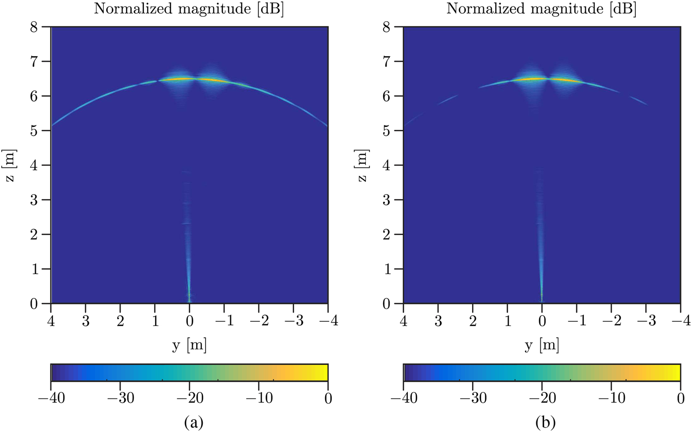
Fig. 11. Radar images along a horizontal cross-section (x = 0) obtained in the second scenario: square MIMO concept (a) and fractal MIMO concept (b).
V. CONCLUSION
MIMO radar concepts based on fractal antenna arrays have been presented in this contribution. It has been shown that array geometries based on the Fudgeflake fractal and the Gosper island fractal are very suitable to improve the angular resolution and to reduce the side lobe level of MIMO radar systems, compared to antenna configurations based on two linear arrays. Furthermore, the two fractals have been combined in order to increase the flexibility of possible realizations concerning the number of transmitting and receiving antennas. The good side lobe suppression and the improved angular resolution have been confirmed by broadband radar measurements for a fractal MIMO concept with 21 transmitting and 21 receiving antennas.
 Christoph Dahl received his Master of Science degree in Electrical Engineering and Information Technology from the Ruhr-University Bochum, Bochum, Germany, in 2012; and he is currently working toward the Ph.D. degree. Since 2012, he has been a Research Assistant with the Institute of Microwave Systems, Ruhr-University Bochum. His current fields of research are concerned with antenna arrays and MIMO radar.
 Michael Vogt received the Dipl.-Ing. degree in Electrical Engineering and the Dr.-Ing. degree from the Ruhr-University Bochum, Germany, in 1995 and 2000, respectively. In 2008, he qualified as a university lecturer at the same location (Habilitation). From 1995 to 2016, he was with the High Frequency Engineering Research Group, and since 2016 he is working at the Institute of Electronic Circuits, both also at the Ruhr-University Bochum. His main areas of research are microwave and ultrasound imaging and measurement techniques, antennas, signal and image processing, and high-frequency electronics. In 2007, he joined Krohne Messtechnik GmbH, Duisburg, Germany, as an R&D scientist, where he is working on electromagnetic level measurement systems, ultrasonic flowmeters, and sensor systems.
 Ilona Rolfes received the Dipl.-Ing. and Dr.-Ing. degrees in Electrical Engineering from the Ruhr-University Bochum, Bochum, Germany, in 1997 and 2002, respectively. From 1997 to 2005, she was with the High Frequency Measurements Research Group, Ruhr-University Bochum, as a Research Assistant. From 2005 to 2009, she was a Junior Professor with the Department of Electrical Engineering, Leibniz Universitaet Hannover, Hannover, Germany, where in 2006, she became Head of the Institute of Radiofrequency and Microwave Engineering. Since 2010, she has been leading the Institute of Microwave Systems, Ruhr-University Bochum. Her fields of research concern high-frequency measurement methods for vector network analysis, material characterization, and noise characterization of microwave devices, as well as sensor principles for radar systems and wireless solutions for communication systems.


