2. TOTAL EXPORTS AND IMPORTS

Chile continues to be mainly a mining export economy. After independence the main products exported by Chile were wheat, silver and copper. Wheat was Chile’s main agricultural commodity until 1879, although it never surpassed the share of mining exports. From 1880 until the Great Depression, the leading Chilean export was saltpetre, or potassium nitrate (Butelmann et al. Reference Butelmann, Cortes-Douglas and Videla1981). Between 1906 and 1910, nitrates comprised 75 per cent of total exports, and direct taxes on exports accounted for 58 per cent of fiscal revenues (Meller Reference Meller1998).

It should be noted that after independence, Chile maintained its former colonial markets with neighbouring countries, together with the new markets of the United Kingdom and the east coast of the United States; which demanded a huge quantity of products due to their economic expansion during the Industrial Revolution. In addition, taking advantage of the fall in trade costs and the expansion of new settler economies, new markets were added: the west coast of the United States and Australia (Collier and Sater Reference Collier and Sater2004).

The war with Peru and Bolivia between 1879 and 1883 was a dramatic turning point for the Chilean economy. The occupation of the northern regions allowed Chile to expand nitrate production (and nitrate exports), and the political instability of its neighbours broke the former colonial trade networks. Exports underwent a severe concentration process, both of product and of market destination (nitrates and the United Kingdom, respectively). By the end of the mining cycle, just four countries imported more than 90 per cent of total Chilean exports (Great Britain, the United States, France and Germany), while other countries played a secondary role, specifically Chile’s existing trade with its South American neighbours (Carreras-Marín et al. Reference Carreras-Marín, Badia-Miró and Peres Cajías2013).

2.1. The Main Sources

As Mamalakis (Reference Mamalakis1978) states, Chile has a broad collection of trade, current account and balance-of-payments statistics. The most important primary source of trade and balance-of-payments statistics for the pre-1925 years comprises the publications of the statistical and census bureau (Dirección General de Estadistica). The report of the «Societe des Nations» (1928: pp. 201-203), indicated that prior to 1916, import values for Chile were official values that commenced in 1897 and were revised every 5 years to obtain a better adjustment to real values. After 1916, the Chilean statistics comprised «declared values». Export values were declared free on board, «a precio corriente de plaza». From 1925 onwards, the reports of the Central Bank became the main source of information.

Díaz et al. (Reference Díaz, Rolf and Wagner2016) provide figures for total exports and imports by splicing various sources. The original trade data came from official sources and were reported in various units of account provided by the following sources (all of them were converted to current dollars):

• ∙ 1810-1844: based on estimates provided by Rector (Reference Rector1985) and interpolated with data from Ibáñez (Reference Ibáñez1912). Data for this period are scarce and unreliable, especially when compared to the later period, so this indicator should be treated as provisional. However, general trends of production, the foreign trade statistics of partner countries and the figures provided by Salazar (2009), taken together corroborate consideration of these numbers as reasonable guesstimates.

• ∙ 1844-1861: the data came from Ibáñez (Reference Ibáñez1912) in current pesos and were converted to dollars with the exchange rate of Díaz et al. (Reference Díaz, Rolf and Wagner2016).

• ∙ 1862-1925: the data came from Oficina Central de Estadística (OCE) (1925). The original data were in 6d pesos; «a fictional unit of constant gold content», as Llona (2012) put it, and were converted to dollars with the exchange rate of Díaz et al. (Reference Díaz, Rolf and Wagner2016).

• ∙ 1926-1930: Servicio Nacional de Estadísticas y Censos de Chile SNECCh (1930). The original data were in 6d pesos.

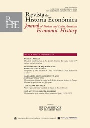
Most of the international databases used reported data for the total imports and exports of Chile, broadly speaking, although the original sources are diverse. Federico and Tena-Junguito (Reference Federico and Tena-Junguito2016) considered the figures of Braun et al. (Reference Braun, Braun, Briones, Díaz, Lüders and Wagner2000) in current dollars, for the period 1810-1938. For total exports in U.S. dollars, Montevideo-Oxford Latin American Database (MOXLAD) (2011) considered Palma’s (Reference Palma1979) growth rate of exports in pounds sterling, for the period 1900-1905. For the rest of the period, they considered Hofman’s (Reference Hofman2000) figures. Imports from MOXLAD (2011) are also taken from Hofman (Reference Hofman2000). Barbieri and Keshk (Reference Barbieri and Keshk2012) and Barbieri et al. (Reference Barbieri, Keshk and Pollins2009) showed total import and total exports in U.S. dollars from secondary sources. They show some discrepancies with the other databases reported, especially prior to 1895. RICardo (2016) also shows data for total exports and imports of Chile in local currency and in pounds sterling. When we apply the exchange rate suggested by Federico and Tena-Junguito (Reference Federico and Tena-Junguito2016) to convert trade figures into current dollars, some discrepancies with the previous figures appear (see Figures 1 and 2).

FIGURE 1 TOTAL EXPORTS OF CHILE, 1845-1938 ($U.S. CURRENT). Sources: Díaz et al. (Reference Díaz, Rolf and Wagner2016), Barbieri et al. (Reference Barbieri, Keshk and Pollins2009), RICardo (2016) and MOXLAD (2011).

FIGURE 2 TOTAL IMPORTS OF CHILE, 1845-1938 ($U.S. CURRENT). Sources: Díaz et al. (Reference Díaz, Rolf and Wagner2016), Barbieri et al. (Reference Barbieri, Keshk and Pollins2009), RICardo (2016) and MOXLAD (2011).

For the period before 1880, RICardo (2016) and Díaz et al. (Reference Díaz, Rolf and Wagner2016) show a close similarity because they used the same original sources. For subsequent years, through the 1880s and the beginning of the 20^th century, RICardo (2016) shows a stagnation in export and import figures. On the other hand, Díaz et al. (Reference Díaz, Rolf and Wagner2016) and Barbieri and Keshk (Reference Barbieri and Keshk2012) show a similar pattern after 1895 and a positive trend during the early 1900s and 1910s. In most of the series, although we observe a peak in 1910, the levels reached were below the levels of the 1920s. However, MOXLAD (2011) figures show big differences before World War I, with nitrate expansion pushing exports to their maximum in 1910, at similar levels to those reached during the 1920s.

As all the series considered reported the same original sources, discrepancies must come either from differences in the exchange rate used in the conversion, or from differences in the treatment of the unit of account reported in the source. As we have said, official Chilean trade figures were reported using «a fictional unit of constant gold content», and its conversion into current values is not simple (Llona 2012).

Comparing all these sources, we confirm that the best available figures to understand Chilean total trade performance are those provided by Díaz et al. (Reference Díaz, Rolf and Wagner2016). They consider the original local sources with the most widely used exchange rates. They also report the shortcomings assumed, which ensures replicability and the capacity for later improvements. At the same time, other economic indicators and secondary sources observed, for the nitrate cycle, fit quite well with the peak in saltpetre exports just before World War I (WWI).

2.3. Quantum Indexes of Exports and Imports

Implicit quantum indexes can be obtained as the ratio between a value index and a price index. In our case, we will compare the quantum index of exports and imports which results from both price indexes: the one provided by Díaz et al. (Reference Díaz, Rolf and Wagner2016) and that provided by Badia-Miró and Carreras-Marín (Reference Badia-Miró and Carreras-Marín2016). Both exports and imports expanded in quantum during the nitrate cycle, until World War I. It seems clear that the expansion started before the Pacific War and the occupation of the Northern provinces. Quantum growth was also important during the wheat and copper export expansion of the 1860s and 1870s. Nevertheless, the export quantum stagnated during the 1920s, with a higher level of volatility. We also observe a coincidence in the dramatic fall of the Great Depression, where the contraction in quantities was as important as the price collapse.

When observing export quantum (see Figure 3), discrepancies in both series are small because the export price indexes in both sources are quite similar, due to the predominance of saltpetre as the leading export commodity during most of the period, and the use of international prices (non-corrected).

FIGURE 3 EXPORT QUANTUM INDEX, 1850-1938 (1913=100). Sources: Badia-Miró and Carreras-Marín (Reference Badia-Miró and Carreras-Marín2016) and Díaz et al. (Reference Díaz, Rolf and Wagner2016).

The expansion of the import quantum was also important during the second half of the 19^th century, following the expansion of exports (see Figure 4). However, this reached its peak at the beginning of the 20^th century. From then, until the Great Depression, we observe stagnation with a high level of volatility, just as for the export quantum. The impact of the Great Depression on imports quantum was profound, following the evolution of the export quantum and the collapse in export and import prices.

FIGURE 4 IMPORT QUANTUM INDEX, 1850-1938 (1913=100). Sources: Badia-Miró and Carreras-Marín (Reference Badia-Miró and Carreras-Marín2016) and Díaz et al. (Reference Díaz, Rolf and Wagner2016).

Discrepancies between both series are important before the 20^th century, due to differences observed in import prices. In Badia-Miró and Carreras-Marín (Reference Badia-Miró and Carreras-Marín2016), the figures for the 1880s showed higher levels (in 1880, e.g., their figures are nearly double those of Díaz et al. (Reference Díaz, Rolf and Wagner2016)), which also implies a smaller growth rate in quantum during the nitrate expansion. Although the period covered by Díaz et al. (Reference Díaz, Rolf and Wagner2016) is broader and provides a long-run view of trade performance in Chile, the methodology proposed by Badia-Miró and Carreras-Marín (Reference Badia-Miró and Carreras-Marín2016) seems to achieve more accuracy. For these reasons we consider both series in later sections of this paper.

3. CHILEAN TRADE: COMPOSITION, ORIGIN AND DESTINATION

The Chilean official reports of international trade were very detailed concerning the types of tradable goods. However, those reports did not provide a systematic and regular classification that made aggregation and standardisation into homogeneous categories easy, at least, not until the end of the 19^th century (Cuevas Reference Cuevas1901). Díaz et al. (Reference Díaz, Rolf and Wagner2016) made great efforts to compile and provide the shares of exports reclassified into big sectors: Agricultural, Mining, Manufactured and Others. These figures could then be transformed into current dollars, multiplying the shares by the total exports value. To build this series, they considered the following sources:

• ∙ 1844-1869: shares from Carmagnani (Reference Carmagnani1971: Appendix 10).

• ∙ 1870-1930: shares from Kirsch (Reference Kirsch1977: pp. 161-162) and Butelmann et al. (Reference Butelmann, Cortes-Douglas and Videla1981: Table 8).

As can be observed in Figure 5, the main exports of Chile between 1844 and 1940 were mineral products, especially copper and nitrate.

FIGURE 5 CHILEAN EXPORTS COMPOSITION, 1844-1940. Sources: Díaz et al. (Reference Díaz, Rolf and Wagner2016).

Regarding the main destinations for Chilean exports, the conventional picture of the British market as the main destination of Chilean exports during the 19^th century, does not appear to be well founded. As Llona-Rodríguez (Reference Llona-Rodríguez2012) has pointed out, between 1870 and 1903, the official reports registered the destination of exports in terms of the «destination of the vessel». This procedure does not take into account the problem of transhipment: ships going to London, for example, might have carried cargoes whose final destination was France, Germany or other Mediterranean ports. For the years 1902 and 1903, Estadística Comercial published both the destination of the vessel and final destination of the shipment. Starting in 1904, the destination of exports seems to be computed in terms of the final destination of the shipment. The share of exports to Britain is greatly reduced when using this second accounting method. From 1914 to 1921 and from 1929 to 1935, a large percentage of nitrate exports were a la orden, meaning without destination at the time of the shipment (Llona-Rodríguez Reference Llona-Rodríguez2012: p. 8). Nevertheless, most of the authors who have worked on this topic assume the Chilean statistics to be reliable. According to Bulmer-Thomas (Reference Bulmer-Thomas2003: Table 3.6), in 1913 the main destinations of Chilean exports were the United Kingdom (38.9 per cent), Germany (21.5 per cent), the United States (21.3 per cent) and France (6.2 per cent). Therefore, although it is plausible to suppose that Europe was the main market for Chilean products during the export-led growth model, the real size of the demand from each country is still open to debate.

As for imports, the Chilean official reports of international trade did not provide a systematic and regular classification that aggregated imports by standardised categories, until the end of the 19^th century. To overcome this, Díaz et al. (Reference Díaz, Rolf and Wagner2016) also compiled shares of imports by sector, classified as Agricultural, Mining, Manufactured and Others. As before, when these shares are multiplied by the total import values, we obtain the levels in current dollars. The sources are:

• ∙ 1844-1910: shares of Carmagnani (Reference Carmagnani1971: Appendix 9).

• ∙ 1911-1966: shares of Díaz and Wagner (Reference Díaz and Wagner2004), based on official reports.

During the period 1844-1940, the main imports of Chile were manufactured goods and coal (Figure 6).

FIGURE 6 CHILEAN IMPORTS COMPOSITION, 1844-1940. Source: Díaz et al. (Reference Díaz, Rolf and Wagner2016).

Ducoing and Tafunell (Reference Ducoing and Tafunell2013) discuss the accuracy of the manufactured imports figures, checking the Chilean reports against official trade statistics from Germany, the United States and Great Britain. They conclude that, although problems in goods classification persist, both series show a similar trend. Nevertheless, it is not easy to identify the origin of Chilean imports. Between 1870 and 1903, the official source, Estadística Comercial, assigned imports to the country of the port of origin of the vessel, while from 1904, imports were allocated according to the country of origin of the goods (when it was known). In other cases, the former rule was applied (Llona-Rodríguez Reference Llona-Rodríguez2012).

With the above-mentioned caveat in mind, Table 1 shows a reduction in the share of British imports and an increase in the prominence of Germany and the United States, as import suppliers to Chile, between 1880 and 1913.

TABLE 1 CHILEAN IMPORTS BY ORIGIN AS PERCENTAGE OF TOTAL IMPORTS

Sources: 1870-1900, Estadística Comercial, selected years; 1913, Bulmer-Thomas (Reference Bulmer-Thomas2003: Table 3.7).

4. ACCURACY OF FIGURES ON CHILEAN BILATERAL TRADE WITH ITS MAIN PARTNERS

Allen and Ely (Reference Allen and Ely1953) and Morgernstern (Reference Morgernstern1963) criticised the use of foreign trade statistics sources, due to their low level of accuracy when comparing different sources recording the same flow (imports of country A from country B should be the same as the exports of country B to country A). The criticisms in these works were later qualified by Federico and Tena-Junguito (Reference Federico and Tena-Junguito1991) and Tena-Junguito (Reference Tena-Junguito1991), who claimed that foreign trade sources could be a useful tool for the study of economics history before World War II, if the shortcomings in geographical and sectorial assignment were considered. Other works have focused on the study of Latin American foreign trade statistics. Authors such as Carreras-Marín and Badia-Miró (Reference Carreras-Marín and Badia-Miró2008)Footnote ⁴ , validate the use of this source and point out its superior quality owing to a better geographical assignment. Other authors have deeply analysed and validated specific countries’ statistics, such as Argentina (Tena-Junguito and Willebald Reference Tena-Junguito and Willebald2013; Carreras-Marín and Rayes Reference Carreras-Marín and Rayes2015), Uruguay (Bonino-Gayoso et al. Reference Bonino-Gayoso, Tena-Junguito and Willebald2015) and Brazil (Absell and Tena-Junguito Reference Absell and Tena-Junguito2016). Morgernstern (Reference Morgernstern1963) quantifies the level of accuracy of a country thus:

$$I_{{ij}} \, {\equals}\, {{X_{{ij}} } \over {M_{{ji}} }}\cdot100$$

where I _ij is the Morgernstern index, X _ij the exports of country i to country j and M _ji the imports of country j from country i. Discrepancies found between the industrialised countries were huge; most of the 25 per cent was expected, due to differences between Cost, Insurance and Freight or Free on Board valuations, and with unexpected signs. Later, Federico and Tena-Junguito (Reference Federico and Tena-Junguito1991) consider geographical assignment problems and correct this index with a regional index which includes the sum of bilateral imports and exports of both sources. The results obtained by these authors, as we have said, substantially reduce the levels of inaccuracy. Their method is expressed thus:

$$FT_{{ij}} \, {\equals}\, {{\sum^ X_{{ij}} } \over {\sum^ M_{{ji}} }}\cdot100$$

where FT _ij is the Federico and Tena index, X _ij are the exports of country i to country j and M _ji the imports of country j from country i. This equation could equally consider whole countries or regions.

If we compute the Morgernstern index for Chile and its main trade partners (namely the United States, the United Kingdom, Germany, Belgium, France, Argentina and Bolivia), we observe a clear pattern of accuracy, worsening around the end of the 1920s and 1930s, in most cases (see Figure 7). Exchange rate volatility associated with the Great Depression could explain most of the discrepancies. However, we observed better results when comparing trade with the United States, the United Kingdom, France and Argentina before WWI, during the nitrate expansion after the Pacific War. We could also include Germany in this group, except for the years around 1880 when discrepancies arise. The case of Belgium has to be considered separately because we observe huge discrepancies during most of the period. The reason behind that (and the lower level of trade reported by Belgium) could be related to a bad geographical assignment of the Belgium trade statistics for imports.

FIGURE 7 MORGERNSTERN INDEX FOR CHILEAN EXPORTS TO THEIR MAIN TRADE PARTNERS, 1850-1938. Notes: ARG: Argentina, GER: Germany, BEL: Belgium, FRA: France. Calculation based on sources described in the text. Lines indicate the upper and the lower band for 25 per cent error around 100 which indicate that both sources show the same figures.

When considering Chilean imports and European exports, the accuracy worsened (Figure 8). Only trade with the United Kingdom and the United States seem to fit quite well. Germany and France joined Belgium in the group of countries with poor levels of accuracy. We can confirm that when we considered exports of these countries to the whole of South America, the huge discrepancies observed when considering bilateral trade, disappeared (so these were mainly due to bad geographical assignment, as Carreras-Marín and Badia-Miró (Reference Carreras-Marín and Badia-Miró2008) pointed out). At the same time, these results confirm our hypothesis that the Chilean sources were good enough to be used.

FIGURE 8 MORGERNSTERN INDEX FOR CHILEAN IMPORTS TO THEIR MAIN TRADE PARTNERS, 1850-1938. Notes: ARG: Argentina, GER: Germany, BEL: Belgium, FRA: France. Calculation based on sources described in the text. Lines indicate the upper and the lower band for 25 per cent error around 100 which indicate that both sources show the same figures.

We also obtained the Federico and Tena index for the accuracy of Chilean exports to their main European partners (with and without the United States). In this case, the results do not confirm the hypothesis that some of the discrepancies could be explained by bad geographical assignments. That is, Chilean trade statistics did not suffer from bad geographical assignment, while previous results would confirm that European trade statistics did suffer from this problem. Figure 9 shows that only a few years exhibited discrepancies lower than the 25 per cent threshold assumed by the authors. Although we have not considered other European countries, such as Spain, Italy or The Netherlands, we could assume that the sample is representative of most European trade. Other possible explanations for these discrepancies could be related to differences between domestic and international prices or high trade costs that were not reported. When we repeat the exercise considering only the European sample or other South American countries, the results are similar and the conclusions are the same.

FIGURE 9 TENA INDEX FOR CHILEAN EXPORTS WITH THEIR MAIN TRADE PARTNERS, 1850-1938. Note: Calculation based on sources described in the text.

By comparison, when we observe Figure 10, we can confirm that Chilean imports and European exports were very similar, assuming the differential of 25 per cent, at least for the years before World War I. The Federico and Tena index performs better when we consider only Europe, at least, for the figures before the 1920s. This result confirms the explanation of bad geographical assignment in some European sources. Moreover, huge problems arose during the Great Depression, jointly with the lack of availability of data in Europe and the United States during the wars. By contrast, Chilean trade statistics are available for the whole period.

FIGURE 10 TENA INDEX FOR CHILEAN IMPORTS WITH THEIR MAIN TRADE PARTNERS, 1850-1938. Note: Calculation based on sources described in the text.

To sum up, the accuracy in matching foreign trade statistics supports the view that the use of Chilean foreign trade statistics to analyse Chilean trade is acceptable. However, discrepancies are higher for imports than for exports, because problems related to geographical assignment are significant, specifically for European countries. Moreover, we observe important valuation problems during the 1920s, after WWI.

5. FINAL REMARKS

Chilean foreign trade statistics are usually considered one of the most reliable sets of figures in Latin America. We discuss most of the existing total import and export figures used in works focused on Chile. In all cases, the original data come from the Chilean official source of foreign trade statistics and the existing discrepancies among them lie in the exchange rate used (local currency to $U.S. or to pounds sterling), or in the price index considered to convert current figures to constant figures. Accuracy tests partially confirm the reliability of bilateral data, especially when we assume the existence of some problems related to geographical assignments.

Above all, these figures confirm the high impact of exports on economic growth, especially during the nitrate era, due to the purchasing power of exporters alongside the expansion of aggregate exports, the downward trend in import prices (which is still being debated), and the high level of fiscal revenues.

By contrast, import price index series (and terms of trade) are still a subject of debate, and the existing figures show very different patterns, especially for import prices during the nitrate cycle. If we observe the main trends, there is a rebound in export prices, from the end of the 19^th century, associated to the saltpetre expansion. Import prices followed a downward trend, which started in the mid-19^th century and lasted until World War I, after which prices became stagnant during the 1920s, until the arrival of the Great Depression.