


1 Introduction
We study a new pension contract that operates in the accumulation phase of a pension scheme. It can be used by an insurance company to smooth the investment return for customers. In contrast to traditional with-profits products, it has a transparent structure and a clearly defined rule for bonus distribution. We compare the new contract to another two similar contracts, which have been studied intensively in previous papersFootnote 1 . Our results show that the new contract is a more attractive contract for a customer under the Cumulative Prospect Theory, which suggests that guarantees should be included in pension contracts.
Pension saving and investment play an important role in an individual’s lifetime wealth management. Thanks to the development of science and health care, people live much longer than before. In order to have a decent lifestyle in retirement, people should have sufficient savings before they are out of the workforce. As Samuelson (Reference Samuelson1958) suggests, people should save some of their income during their working years for their retirement.
For customers, choosing a pension contract is making a decision under uncertainty. Hence, decision theory is often used in designing pension and insurance contracts. One widely used decision theory is Expected Utility Theory (Von Neumann & Morgenstern, Reference Von Neumann and Morgenstern1944) which is a dominant theory in the last century to explain individuals’ behaviour under uncertainty. The calculation of expected utility is easy to understand and implement. Specifically, the expected utility of investment is just the sum of the utility of each possible outcome weighted by its probability. However, there are critics of Expected Utility Theory (henceforth called EUT) as it fails to explain people’s behaviour in some cases. Tversky & Kahneman (Reference Tversky and Kahneman1992) summarise five violations of EUT in explaining people’s behaviour under uncertainty. The most famous examples are Allais’ (Reference Allais1953) paradox and Ellsberg’s (Reference Ellsberg1961) paradox.
A new theory to describe individual’s behaviour, Cumulative Prospect Theory (and its original version of Prospect TheoryFootnote 2 ), is becoming more popular in evaluating how people make a decision under uncertainty. Cumulative Prospect Theory (henceforth called CPT) is proposed by Tversky & Kahneman (Reference Tversky and Kahneman1992) to explain the choice made by people violating the standard EUT. The most distinct part of CPT is that it values outcomes based on gains or losses relative to a reference level of wealth rather than on the absolute value of the wealth at retirement. In addition, people tend to overvalue small probabilities and undervalue moderate and high probabilities. Instead of using real-world probability, CPT uses a cumulative weighting function which is a distortion of the probability.
This paper focusses on the accumulation of the pension savings. In this sense, the pension contract works as a long-term saving product which helps people accumulate money during the working years, and its proceeds can be used to provide them with an income after their retirement. How to design an attractive pension product for customers is of significance to the product development department of life insurance companies and pension providers. Chen et al. (Reference Chen, Hentschel and Klein2015) suggests there are generally two ways to design a pension contract. One is to solve an optimisation problem for a specific utility theory and reversely design the contract from the optimal strategy. This method has been used by Bruhn & Steffensen (Reference Bruhn and Steffensen2013) to reversely engineer an optimal product under EUT. Hens & Rieger (Reference Hens and Rieger2014) also use this method to approximate the optimal payoff under the Prospect Theory. The other way is to find out the contract that delivers the highest utility value among some contracts on the perspective of the customer. This can be done by calculating the utility of different products using a chosen utility function. The product generating the highest utility is the most attractive one (this is done in Døskeland & Nordahl, 2008 Reference Døskeland and Nordahlb ; Branger et al., Reference Branger, Mahayni and Schneider2010; Chen et al., Reference Chen, Hentschel and Klein2015). Another widely used method is to find the optimal portfolio which gives the largest utility for customers. If one contract exists in the optimal portfolio while the other does not, then the former should be viewed as a more attractive product for customers (see Døskeland & Nordahl, 2008 Reference Døskeland and Nordahla ).
As we design the contract first, the second method is chosen in this paper. Specifically, we compare our new contract against the other two similar contracts as well as a risky asset and a risk-free asset in two methods, finding the contract generates the highest utility and investigating the optimal portfolio under both the CPT and EUT, by assuming customers use a buy-and-hold strategy. As individual pension investors tend not to review their investment holdings frequently, buy-and-hold is a more reasonable investment strategy. The comparison results show that our contract is an attractive contract to a CPT-maximising customer. However, we do not reach the same conclusion for an EUT-maximising customer.
For a CPT investor, Døskeland & Nordahl (2008 Reference Døskeland and Nordahlb ) and Dichtl & Drobetz (Reference Dichtl and Drobetz2011) provide the evidence that investment guarantees increase an investor’s utility. This explains why many traditional pension contracts in the market incorporate guarantees, either in the form of interest rate guarantees or as a sum assured. Hens & Rieger (Reference Hens and Rieger2014) suggest that an optimal structured product should not only have downside protection but also retain the potential of upside return. Their finding is consistent with the design fashion of including a bonus feature into pension contracts. Hence, our new contract is presented as the combination of a ratchet type guarantees and a possible bonus. This kind of structure removes the risk of loss for a policyholders investment and keeps the opportunity to make a positive return.
There are some pension products studied in the literature with a similar structure in terms of ratchet style guarantees, a smoothing mechanism and a possible bonus. They are different from each other mainly because of their bonus determination method. As Zemp (Reference Zemp2011) suggests, most of these products can be grouped into two categories. One is a return-based bonus distribution. For instance, Bacinello (Reference Bacinello2001) determines the bonus by comparing the annual investment return with the guaranteed rate while Haberman et al. (Reference Haberman, Ballotta and Wang2003) use the past 3 years’ average return. The other category is a reserve-based bonus distribution. These contracts generally have a target buffer ratio or a target reserve level for the insurance company, as Grosen & Jørgensen (Reference Grosen and Jørgensen2000) and Hansen & Miltersen (Reference Hansen and Miltersen2002) show. In contrast to these approaches, the bonus determination method of our new contract is to compare the value of a specified investment account and the customer account. It has a well-defined return distribution rule and a transparent product structure.
The remainder of the paper is organised as follows. In section 2, we introduce the new pension contract. The pricing and some characteristics of the new contract are also given in this part. Additionally, two similar pension contracts, one with a similar product structure but without guarantee embeddedFootnote 3 and the other providing similar guarantees but with an entirely different product structureFootnote 4 , are introduced in this part as well. Section 3 compares the new contract with these two contracts under CPT. In section 4, some robustness and sensitivity test is carried out. In order to know how these two contracts perform for an EUT customer, we also provide a comparison of these three contracts under EUT in section 5. The last part of this paper is the conclusion.
2 Product design
Mortality, surrender and expense are not considered in this paperFootnote 5 , as we are more interested in the savings aspect of pension products. Here, the new contract is introduced in detail. A brief introduction of the other two similar contracts is also given in this part.
2.1 Financial market model
It is assumed that the investment takes over a finite time horizon [0, T], where T is a strictly positive integer. There are only two underlying assets in the market. One is the risk-free asset and the other is the risky asset. The risk-free asset can be a government bond while the risky asset could be an equity index. The prices of both assets are available in the market. Pension contracts are derivatives of these two underlying assets. The evolution of the value of the risk-free asset B t is
 $$dB_{t} {\equals}rB_{t} dt,\quad B_{0} {\equals}b$$
where r>0 is the constant risk-free interest rate and b>0 is a constant. The price of the risky asset follows the following geometric Brownian motion.
 $$dS_{t} {\equals}\mu \,S_{t} dt{\plus}\sigma \,S_{t} \,dW_{t} ,\quad S_{0} {\equals}s$$
where the expected growth rate µ, volatility σ and initial value s are positive constants. W is a standard Brownian motion defined on the filtered probability space (Ω,
![]() $${\Bbb F}$$
,(
$${\Bbb F}$$
,(
![]() $${\cal F}$$
t), ℙ). All the perfect market assumptions suggested by Black & Scholes (Reference Black and Scholes1973) hold here. The Black–Scholes model is widely used in literature for the study of insurance and pension contracts, e.g., Døskeland & Nordahl (2008
Reference Døskeland and Nordahlb
), Branger et al. (Reference Branger, Mahayni and Schneider2010) and Bauer et al. (Reference Bauer, Kiesel, Kling and Ruß2006).
$${\cal F}$$
t), ℙ). All the perfect market assumptions suggested by Black & Scholes (Reference Black and Scholes1973) hold here. The Black–Scholes model is widely used in literature for the study of insurance and pension contracts, e.g., Døskeland & Nordahl (2008
Reference Døskeland and Nordahlb
), Branger et al. (Reference Branger, Mahayni and Schneider2010) and Bauer et al. (Reference Bauer, Kiesel, Kling and Ruß2006).
2.2 New contract
The inspiration for the new contract arises from Guilléen et al. (Reference Guilléen, Jørgensen and Nielsen2006). In their paper, they study a pension product with the features of a transparent structure and no embedded guarantee. We refer to this contract as the GJN contract, although it appears to be a contract that is sold in DenmarkFootnote 6 .
The GJN contract enjoys the return from the underlying asset but cannot provide the protection for policyholders against the downside risk if the market performs badly. However, according to the findings of Hens & Rieger (Reference Hens and Rieger2014), incorporating the feature of downside capital protection while keeping the exposure to the upward return makes structured products more attractive. Hence, by modifying the return distribution rule in the GJN contract, we obtain a new pension contract whose value to the customers has a lower bound. In addition, the payoff of the new contract is determined by the performance of a specified asset whose price is known to the public. Along with the clear profit distribution rule, this ensures that the return from the new contract is transparent.
2.2.1 Structure of new contract
Our new contract consists of three accounts: the investment account A, the customer account D and the smoothing account U. The value of the investment account is always equal to the sum of customer account D and smoothing account U. Mathematically,
 $$A_{t} {\equals}D_{t} {\plus}U_{t} ,\quad {\rm for}\,{\rm all}\,\,t\in\left[ {0,T} \right]$$
The investment account A is a notional account which replicates the trend of the risky asset. For simplicity, the customer is assumed to pay a one-off premium P>0 at the start. Then the value of the investment account of this customer is given as:
 $$A_{t} {\equals}P\,{\rm exp}\left[ {\left( {\mu {\minus}{1 \over 2}\sigma ^{2} } \right)\,t{\plus}\sigma W_{t} } \right],\quad {\rm for}\,{\rm all}\,t\in\left[ {0,T} \right]$$
On the expiration date T, the customer will receive all the money in the customer account D. At the end of year n, the nominal value of the customer account increases at a pre-declared guaranteed rate g n (it is generally declared at the beginning of the year, in practice). Apart from this guaranteed return, the customer account is credited an annual bonus which is defined as a fixed proportion α ∈[0, 1] of the excess value of the investment account over the guaranteed value of customer account. The proportion α is generally called the participation rate or distribution ratio. The other part, 1−α of the excess value, goes to the smoothing account U which provides the customer account with the guaranteed return when the market performance is bad. The value of customer account and smoothing account are updated only at the end of each year. The value of the customer account is:
 $$D_{n} {\equals}\left\{ {\matrix{ {P,} & {n{\equals}0,} \cr {\left( {1{\plus}g_{n} } \right)D_{{n{\minus}1}} {\plus}\alpha \,{\rm max}\left[ {A_{n} {\minus}\left( {1{\plus}g_{n} } \right)D_{{n{\minus}1}} ,0} \right],} & {n\in\left\{ {1,2,...,T} \right\}} \cr } } \right.$$
At the end of each year, the customer receives a positive return, or so-called bonus, if the value of the investment account is larger than the value of the customer account in the previous year increased at the guaranteed rate g n ≥0. Otherwise, the bonus is zero and the customer account only increases at the guaranteed rate. According to equations (3)–(5), the value of the smoothing account is
 $$U_{n} {\equals}\left\{ {\matrix{ {\,\,\,\,\,\,\,\,\,\,\,\,\,\,\,\,\,\,\,\,\,\,\,\,\,\,\,\,\,\,\,\,\,\,\,\,\,\,\,\,\,\,\,\,\,\,\,\,\,\,\,\,\,0,} \hfill & {n{\equals}0,} \hfill \cr {A_{n} {\minus}\left( {1{\plus}g_{n} } \right)D_{{n{\minus}1}} {\minus}\alpha \,{\rm max}\left[ {A_{n} {\minus}\left( {1{\plus}g_{n} } \right)D_{{n{\minus}1}} ,0} \right],} \hfill & {n\in\left\{ {1,2,...,T} \right\}} \hfill \cr } } \right.$$
From equation (6), we can see that the smoothing account can be negative in which case the value of the investment account is less than the customer account.
It is important to note that the value of the customer account or smoothing account is a nominal value. It is not the market value of each account, although the nominal value and the market value have the same initial value and terminal value. There is no cash-flow to the customer account at the end of each year before the maturity date T. The only cash-flow happens at time T when the insurer pays the terminal value D T to the policyholder. The advantage of the contract is that the customers can understand what they receive at the terminal time T. In addition, the investment strategy that replicates their terminal payoff is not, in general, to invest their premium entirely in the risky asset. Thus, the value of the replicating portfolio is not likely to be equal to the value of the customer account before the maturity date T. This is discussed in Guilléen et al. (Reference Guilléen, Jørgensen and Nielsen2006) in relation to the contract that they study.
2.2.2 Terminal value of the customer account
In the following, we give an expression for the terminal value of the customer account. The customer of our new contract receives an annual bonus which can never be negative, as can be seen from equation (5). The annual bonus is the payoff of a 1-year call option with underlying price A n and strikes price K n =(1+g n )D n−1. We let C n denote the payoff of nth year option, i.e.
 $$C_{n} {\equals}{\rm max}\left[ {A_{n} {\minus}\left( {1{\plus}g_{n} } \right)D_{{n{\minus}1}} ,0} \right],\,n\in\left\{ {1,2,...,T} \right\}$$
For simplicity, the guaranteed rate g n is assumed to be a constant value g, i.e., g n =g for n∈{1, 2, … , T}. After recursive substitution of the second part in equation (5), we get
 $$D_{n} {\equals}D_{j} \left( {1{\plus}g} \right)^{{n{\minus}j}} {\plus}\alpha \mathop{\sum}\limits_{i{\equals}j{\plus}1}^n {C_{i} \left( {1{\plus}g} \right)^{{n{\minus}i}} ,\,{\rm for } \ 0 \ \leq j\,\lt\,n\leq T} {\rm \ztbnd }$$
where j∈{0, 1, … , T}. If we let j=0 and n=T, then the value of the customer account at the maturity date is
 $$D_{T} {\equals}D_{0} \left( {1{\plus}g} \right)^{T} {\plus}\alpha \mathop{\sum}\limits_{i{\equals}1}^T {C_{i} \left( {1{\plus}g} \right)^{{T{\minus}i}} } $$
From equation (9), we can separate the value of customer account into two parts. The first part is a pure risk-free bond with the interest rate g and the second part is a series of consecutive forward start 1-year call options (ratchet style). All options begin from the start of the contract but only the first option’s strike price is known at the start. In year n, there are T−n+1 contracts in force and only the strike price of nth option is known. Hence, the terminal value in the customer account depends not only on the participation rate α, guarantee rate g and the contract term T, but also on the paths of
 $\left\{ {A_{n} } \right\}_{{n{\equals}0}}^{T} $
.
$\left\{ {A_{n} } \right\}_{{n{\equals}0}}^{T} $
.
2.2.3 Fair pricing of the contract
In this section, we show how to fairly price this contract and present some of its characteristics. We have shown the payoff of the new contract above. But it is also important for insurers to know the market value of the new contract during its lifetime.
Pricing pension contracts are generally carried out under an equivalent martingale measure (Harrison & Kreps, Reference Harrison and Kreps1979). There are many papers using this method in the pricing of pension contracts, like Bacinello (Reference Bacinello2001), Grosen & Jørgensen (Reference Grosen and Jørgensen2000) and Bauer et al. (Reference Bauer, Kiesel, Kling and Ruß2006).
Let r
f
=e
r
−1 be the discretely compounded annual risk-free interest rate and V
D
(t) denote the market value of the customer account at time t. Discounting the terminal value D
T
back to time 0 under the equivalent martingale measure
![]() $${\Bbb Q}$$
, we get the initial price of this contract. That is
$${\Bbb Q}$$
, we get the initial price of this contract. That is
 $$V^{D} \left( 0 \right){\equals}\left( {{{1{\plus}g} \over {1{\plus}r_{f} }}} \right)^{T} D_{0} {\plus}{\alpha \over {\left( {1{\plus}r_{f} } \right)^{T} }}{\Bbb E}^{{\Bbb Q}} \left( {\mathop{\sum}\limits_{i{\equals}1}^T {{\rm max}\left[ {A_{i} {\minus}\left( {1{\plus}g} \right)D_{{i{\minus}1}} ,0} \right]\left( {1{\plus}g} \right)^{{T{\minus}i}} } } \right)$$
If the expected discounted value of the terminal value in the customer account V D (0), at time 0, is equal to customer’s initial premium P, then this contract is viewed as a fair contract for the customer. We also can price this contract from the perspective of the insurer. The insurer does not put any money into the smoothing account at the start of the contract and will keep the terminal value in the smoothing account which can be positive or negative. For a fair contract, the expected discounted value of the smoothing account is zero. However, as equation (6) shows, valuing the smoothing account is a matter of valuing the customer account first and then subtracting its value from the investment account. That is, V U (0)=A 0−V D (0), where V U (t) is the market value of the smoothing account at time t. Thus, we only need to show the pricing based on the customer account.
Observe from equation (10) that the first component,
 $\left( {{{1{\plus}g} \over {1{\plus}r_{f} }}} \right)^{T} \,D_{0} $
, is the present value of a fixed income asset with the interest rate g. The second part is the present value of a series of the payoffs of call options. The payoff for each of these call options is worth at least zero. Thus we must have g≤r
f
to make this contract fair. As we cannot get a closed form solution for the pricing of the new product due to the path-dependency of the options, Monte Carlo simulation is used to price this contract.
$\left( {{{1{\plus}g} \over {1{\plus}r_{f} }}} \right)^{T} \,D_{0} $
, is the present value of a fixed income asset with the interest rate g. The second part is the present value of a series of the payoffs of call options. The payoff for each of these call options is worth at least zero. Thus we must have g≤r
f
to make this contract fair. As we cannot get a closed form solution for the pricing of the new product due to the path-dependency of the options, Monte Carlo simulation is used to price this contract.
Under a risk-neutral measure ℚ, the value of the investment account can be expressed as
 $$A_{t} {\equals}P\,{\rm exp}\left[ {\left( {r{\minus}{1 \over 2}\sigma ^{2} } \right)t{\plus}\sigma \,W_{t}^{{\Bbb Q}} } \right],\,{\rm for}\,{\rm all}\,\,t\in\left[ {0,T} \right]$$
For a contract with fixed-term T, the guarantee rate g and participation rate α are two parameters under the insurer’s control which could be adjusted to make this contract a fair one. In order to identify the relationship between g and α, we fix the value of one parameter and find out the value of the other which makes the contract fair. Newton’s method is used to solve this problem.
Figure 1 shows the relationship between these two parameters for a 20-year contract with risk-free rate r f =0.04 and volatility σ∈{0.1, 0.2, 0.3}. The participation rate α decreases with the increase of the guarantee rate g. This is intuitive, as the customer should have a lower share of the excess return with the increase of the guaranteed return. If the guaranteed return equals the risk-free rate, then the customer only holds a pure risk-free bond. The figure also shows that the higher the volatility σ, the lower the participation rate α. As the market becomes more volatile, the investment account is more likely to make a loss, the guarantees become more valuable and thus lead to a smaller participation rate.

Figure 1 Relationship between guarantee rate g and participation rate α. T=20 years, r f =0.04 and σ∈{0.1, 0.2, 0.3}.
As we mentioned earlier, the value of the customer account D t tends to be different from the market value of the customer account V D (t) at any time t∈(0,T), though the start value and the terminal value of the two are the same. In order to show how the customer account value and the market value of customer account evolve in different market scenarios, we choose two different scenarios simulated from equation (4). The parameters we used in the simulation are r f =0.04, μ=0.065 and σ=0.15Footnote 7 .
∙ Bull market scenario.
The value of the risky asset mainly follows an upward trend.
∙ Bear market scenario.
The value of the risky asset mainly follows a downward trend.
Figure 2 shows the behaviour of the nominal value of the customer account, the market value of customer account and the investment account value in a bull market scenario. The customer account value D t rises in a step-wise fashion every year. It never decreases due to the guarantee of the participation in the risky asset return, unlike the contract studied in Guilléen et al. (Reference Guilléen, Jørgensen and Nielsen2006). In the first 5 years, the market value of customer account V D (t) follows closely with the investment account A t . In contrast, it follows closely the customer account value D t in the later period of the contract. At the terminal time, V D (T)=D T . In this scenario, the investment account has a much higher terminal value than the customer account.

Figure 2 The behaviour of account balance D t , the market value of customer account V D (t) and investment account A t in bull market. α=0.13, T=20 years, g=0.02, r f =0.04, μ=0.065 and σ=0.15. In the simulation, there are 100 steps in each year.
In Figure 3, the bear market scenario, the market value of customer account V D (t) also tracks closely the investment fund for the first few years and moves along the customer account value during the last few years. But this time the customer account has a much larger terminal value than the investment account. In other words, the customer’s money still increases even when the risky asset performs badly.

Figure 3 The behaviour of account balance D t , the market value of customer account and investment account A t in bear market. α=0.13, T=20 years, g=0.02, r f =0.04, μ=0.065 and σ=0.15. In the simulation, there are 100 steps in each year.
2.2.4 Investment strategy
Rather than investing all of the customer’s premium in the risky asset, the insurer could construct the replicating portfolio to replicate the market value of the customer account. This could mitigate the hedging error to which the former strategy exposes the insurer. The weight in the risky asset, or the Delta of the portfolio, can be calculated by using a Monte Carlo method. Figure 4 shows the average weight of portfolio in the risky asset, which is calculated using a finite difference approximation. We can see that as the contract approaches the maturity date, the weight of the risky asset in the portfolio is decreasing. The hedging portfolio shows a life-style investment strategy. In other words, you should put more money in the risky asset if you are young and hold less in the risky asset when you are old. If the insurer follows the replicating portfolio, then at time T, the value of the replicating portfolio is V D (T)=D T , a.s.

Figure 4 The mean of portfolio weight in the risky asset. It is calculated by simulating 100 paths. α=0.13, T=20 years, r f =0.04, μ=0.065 and σ=0.15.
Suppose the insurer does not follow the replicating portfolio. Instead, they invest all the premium into the risky asset at the start and hold until the maturity. This approach leads to a hedging error, A t −V D (t), which equals the market value of the smoothing account, V U (t). The smoothing account belongs to the insurer, which makes sense as the hedging error is the responsibility of the insurer too. If the insurer chooses not to follow the replicating strategy for the contract, then it should bear the financial consequences, rather than the customers. In this sense, if we are in the bull scenario (Figure 2), the excess investment gains, A T −D T , goes into the smoothing account, which belongs to the insurer. If we are in the bear scenario as Figure 3 shows, the insurer needs to use its own money to meet the full terminal value of the customer account D T by injecting the amount, D T −A T , at time T.
2.3 GJN contract
In this part, we briefly introduce the pension contract which is discussed in Guilléen et al. (Reference Guilléen, Jørgensen and Nielsen2006), as we will compare the new contract against this contract in next section. The structure of GJN contracts is similar to our new contract. The only difference is GJN contract lacks protection for the downside risk. Specifically, each year, the value of customer account increases at a constant discretely compounded reference policy interest rate r
p
. The reference policy interest rate r
p
in the GJN contract is analogous to the guaranteed rate g in the new contract. In addition to this, the policyholder can receive a fixed portion of the difference between the value of the investment account A
n
and the value of the previous year’s customer account
 $D_{{n{\minus}1}}^{'} $
accumulated at the reference policy interest rate r
p
. Mathematically, the development of the customer account in the GJN contract is expressed as
$D_{{n{\minus}1}}^{'} $
accumulated at the reference policy interest rate r
p
. Mathematically, the development of the customer account in the GJN contract is expressed as
 $$D{\rm '}_{n} {\equals}\left\{ {\matrix{ {P,} & {n{\equals}0,} \cr {\left( {1{\plus}r_{p} } \right)D{\rm '}_{{n{\minus}1}} {\plus}\alpha {\rm '}\left[ {A_{n} {\minus}\left( {1{\plus}r_{p} } \right)D{\rm '}_{{n{\minus}1}} } \right],} & {n\in\{ 1,...,T\} } \cr } } \right.$$
where the constant α′∈[0, 1] is the participation rate. Similar to the new contract, the value of the smoothing account in GJN contract is U′ n =A n −D′ n .
It is worth mentioning here that if the investment account A n has a lower value than the guaranteed value of customer account, the value of [A n −(1+r p )D′ n−1] can be negative. That is to say that the customer account is credited with a negative bonus and the value of customer account decreases. This is the critical difference between the GJN contract and the new contract. In the new contract, the customer will never have a loss in the customer account.
For both contracts, the smoothing account accumulates wealth when the market performance is good and gives the money back when the market performs badly. Ideally, the smoothing account is expected to even out the short-term fluctuations over a long term. In some situations when the market returns are too bad, the smoothing account in both contracts would end up with a negative value, i.e., a loss. In some other situations, the smoothing account ends up with a positive balance and generates profit for the insurance company. As we discussed before, this is only a true profit or loss if the company does not follow the replicating strategy for the terminal value of the customer account.
2.4 DN contract
Døskeland & Nordahl (2008
Reference Døskeland and Nordahlb
) introduce a contract which consists of four accounts: the investment account A″
t
, customer account L
t
, bonus account I
t
and insurer account E
t
. For easier comparison, we change the wording and notation of this contract. Specifically, at time 0, the customer pays the premium P into the customer account, i.e., L
0=P. Different from the other two contracts, the insurer also needs to put money in at the outset for this contract and the money is deposited into the insurer account. The money in the customer account and insurer account are invested into the risky asset. The market value of this investment is denoted by the investment account A″
t
. That the insurer does not follow the replicating portfolio is a critical distinction for the DN contract. The proportion of the premium relates to the value of the investment account at the start,
 $\psi {\equals}{P \over {A{\rm ''}_{0} }}$
, is called the capital structure parameter. The initial value of the insurer account is
$\psi {\equals}{P \over {A{\rm ''}_{0} }}$
, is called the capital structure parameter. The initial value of the insurer account is
 $E_{0} {\equals}{{1{\minus}\psi } \over \psi }P$
. Thus, A″0=L
0+E
0. Additionally, the bonus account has an initial value I
0=0.
$E_{0} {\equals}{{1{\minus}\psi } \over \psi }P$
. Thus, A″0=L
0+E
0. Additionally, the bonus account has an initial value I
0=0.
The mathematical expression of the customer account L t , the bonus account I t and the insurer account E t for t=1, 2, … , T are given as
 $$L_{t} {\equals}\left\{ {\matrix{ {A{\rm ''}_{t} ,} \hfill & {{\rm if }\,A{\rm ''}_{t} \leq L_{{t{\minus}1}} \left( {1{\plus}g{\rm ''}} \right)} \hfill \cr {L_{{t{\minus}1}} \left( {1{\plus}g{\rm ''}} \right),} \hfill & {{\rm otherwise }\,A{\rm ''}_{t} \leq \left( {L_{{t{\minus}1}} {\plus}E_{{t{\minus}1}} } \right)\left( {1{\plus}g{\rm ''}} \right){\plus}I_{{t{\minus}1}} } \hfill \cr {L_{{t{\minus}1}} \left( {1{\plus}g{\rm ''}} \right){\plus}\psi \eta \left( {1{\minus}\theta } \right)} \hfill & {} \hfill \cr { \cdot \left( {A{\rm ''}_{t} {\minus}\left[ {\left( {L_{{t{\minus}1}} {\plus}E_{{t{\minus}1}} } \right)\left( {1{\plus}g{\rm ''}} \right){\plus}I_{{t{\minus}1}} } \right]} \right),} \hfill & {{\rm if }\,A{\rm ''}_{t} \,\gt\,\left( {L_{{t{\minus}1}} {\plus}E_{{t{\minus}1}} } \right)\left( {1{\plus}g{\rm ''}} \right){\plus}I_{{t{\minus}1}} } \hfill \cr } } \right.$$
 $$I_{t} {\equals}\left\{ {\matrix{ {0,} \hfill & {{\rm if }\,A{\rm ''}_{t} \leq L_{{t{\minus}1}} \left( {1{\plus}g{\rm ''}} \right){\plus}E_{{t{\minus}1}} } \hfill \cr {A{\rm ''}_{t} {\minus}L_{{t{\minus}1}} \left( {1{\plus}g{\rm ''}} \right){\minus}E_{{t{\minus}1}} ,} \hfill & {{\rm otherwise}\,{\rm }A{\rm ''}_{t} \leq L_{{t{\minus}1}} \left( {1{\plus}g{\rm ''}} \right){\plus}E_{{t{\minus}1}} {\plus}I_{{t{\minus}1}} } \hfill \cr {I_{{t{\minus}1}} ,} \hfill & {{\rm otherwise }\,A{\rm ''}_{t} \leq \left( {L_{{t{\minus}1}} {\plus}E_{{t{\minus}1}} } \right)\left( {1{\plus}g{\rm ''}} \right){\plus}I_{{t{\minus}1}} } \hfill \cr {I_{{t{\minus}1}} {\plus}\psi \eta \theta } \hfill & {} \hfill \cr { \cdot \left( {A{\rm ''}_{t} {\minus}\left[ {\left( {L_{{t{\minus}1}} {\plus}E_{{t{\minus}1}} } \right)\left( {1{\plus}g{\rm ''}} \right){\plus}I_{{t{\minus}1}} } \right]} \right),} \hfill & {{\rm if }\,L_{t} \,\gt\,L_{{t{\minus}1}} \left( {1{\plus}g{\rm ''}} \right){\plus}E_{{t{\minus}1}} \left( {1{\plus}g{\rm ''}} \right){\plus}I_{{t{\minus}1}} } \hfill \cr } } \right.$$
 $$E_{t} {\equals}A{\rm ''}_{t} {\minus}L_{t} {\minus}I_{t} $$
where η∈[0, 1] is the customer share of the profits and θ∈[0,1] is the proportion of declared bonuses credited to the bonus account.
The customer receives at the expiration date D″ T is the sum of the value of the customer account L T and the bonus account I T . In the paper of Døskeland & Nordahl (2008 Reference Døskeland and Nordahlb ), the insurer is allowed to go into bankruptcy (A″ t <L t−1(1+g″)), in which case the terminal payoff to the customers is the value of the investment account at the time of bankruptcy, accumulated at the risk-free rate to the maturity date of the contract. That is
 $$D{\rm ''}_{T} {\equals}A_{\tau } \left( {1{\plus}r_{f} } \right)^{{T{\minus}\tau }} $$
where τ∈(0,T) is the bankruptcy time. As the customer account is only updated at the end of each year, the bankruptcy time can only be an integer time. It is noted that in the case of bankruptcy, the annual guarantees cannot be met. In other words, customers may receive less than the guaranteed value.
3 Comparison under CPT
In this part, we compare the new contract with the GJN contract and the DN contract in detail. The results provide the evidence that the new contract is more preferable than the other two. CPT is used in this section to compare these three contracts. The comparison is based on the results of Monte Carlo simulations. An alternative test using EUT is given in section 5.
3.1 CPT
Now we examine the performance of these three contracts under the behavioural model, CPT. Compared to EUT, CPT assumes that a person values an investment by gains or losses rather than the terminal wealth. The gains and losses are calculated by comparing the terminal value of an investment to a reference point which is often the current wealth. In this paper, we choose the initial investment, the premium P, as the reference point. If the terminal value the customer received
 $D_{T}^{{\rm {\asterisk}}} $
(D
T
,
$D_{T}^{{\rm {\asterisk}}} $
(D
T
,
 $D_{T}^{\prime} $
',
$D_{T}^{\prime} $
',
 $D_{T}^{\prime\prime} $
') is smaller than the premium, i.e.,
$D_{T}^{\prime\prime} $
') is smaller than the premium, i.e.,
 $X{\equals}D_{T}^{{\rm {\asterisk}}} {\minus}P\,\lt\,0$
, the outcome is viewed as a loss. Otherwise, it is a gain. An investment consisting of m outcomes of losses and n outcomes of gains is expressed as a risk prospect f=(x
−m
, p
−m
; x
−m
+
1, p
−m
+
1; … ; x
i
, p
i
; … ; x
n−1, p
n−1; x
n
, p
n
), where x
i
is a potential outcome of the prospect and p
i
is the corresponding probability for i={−m,−m+1, 0, … n−1, n}. CPT evaluates gains and losses separately, and the overall utility is the sum of the utility of the positive part f+ and the negative part f
−.
$X{\equals}D_{T}^{{\rm {\asterisk}}} {\minus}P\,\lt\,0$
, the outcome is viewed as a loss. Otherwise, it is a gain. An investment consisting of m outcomes of losses and n outcomes of gains is expressed as a risk prospect f=(x
−m
, p
−m
; x
−m
+
1, p
−m
+
1; … ; x
i
, p
i
; … ; x
n−1, p
n−1; x
n
, p
n
), where x
i
is a potential outcome of the prospect and p
i
is the corresponding probability for i={−m,−m+1, 0, … n−1, n}. CPT evaluates gains and losses separately, and the overall utility is the sum of the utility of the positive part f+ and the negative part f
−.
 $$V\left( f \right){\equals}V\left( {f^{{\plus}} } \right){\plus}V\left( {f^{{\minus}} } \right){\equals}\mathop{\sum}\limits_{i{\equals}0}^n {\pi _{i}^{{\plus}} v\left( {x_{i} } \right){\plus}\mathop{\sum}\limits_{i{\equals}{\minus}m}^0 {\pi _{i}^{{\minus}} v\left( {x_{i} } \right),{\rm }{\minus}m\,\lt\,i\,\lt\,n} } $$
where v(x
i
) is the value function of outcome x
i
and
 $\pi _{i}^{{{\plus}({\minus})}} $
the decision weight of this outcome. The value function shows how the individual values the outcomes. The decision weight is calculated by weighting function w: [0, 1]→[0, 1] (Choquet, Reference Choquet1954) which is a distortion of real probability. The weighting function describes how people deal with probabilities. For a positive outcome x
j
, the decision weight
$\pi _{i}^{{{\plus}({\minus})}} $
the decision weight of this outcome. The value function shows how the individual values the outcomes. The decision weight is calculated by weighting function w: [0, 1]→[0, 1] (Choquet, Reference Choquet1954) which is a distortion of real probability. The weighting function describes how people deal with probabilities. For a positive outcome x
j
, the decision weight
 $\pi _{j}^{{\plus}} $
is
$\pi _{j}^{{\plus}} $
is
 $$\pi _{j}^{{\plus}} {\equals}w\left( {p_{j} {\plus}...{\plus}p_{n} } \right){\minus}w\left( {p_{{j{\plus}1}} {\plus}...{\plus}p_{n} } \right)$$
On the other hand, the decision weight for a negative outcome x i is:
 $$\pi _{i}^{{\minus}} {\equals}w\left( {p_{{{\minus}m}} {\plus}...{\plus}p_{i} } \right){\minus}w\left( {p_{{{\minus}m}} {\plus}...{\plus}p_{{i{\minus}1}} } \right)$$
The value function used in this paper is proposed by Tversky & Kahneman (Reference Tversky and Kahneman1992):
 $$v\left( x \right){\equals}\left\{ {\matrix{ {x^{\beta } ,\,{\rm if}\,x\geq 0} \cr {{\minus}\lambda \left( {{\minus}x} \right)^{\beta } ,\,{\rm if}\,x\,\lt\,0} \cr } } \right.$$
where λ=2.25 and β=0.5. λ>1 is the loss aversion parameter, which shows individuals are much more sensitive to losses than gains. β is the sensitivity of customers to the increasing gains or losses. Prelec (Reference Prelec1998) proposes a one parameter weighting function, namely the Prelec’s weighting function:
 $$w\left( p \right){\equals}e^{{{\minus}\left( {{\minus}{\rm ln}p} \right)^{\varphi } }} $$
Døskeland & Nordahl (2008 Reference Døskeland and Nordahlb ) suggest Prelec’s weighting function is based on behavioural axioms rather than mathematical convenience. In this section, we follow Døskeland & Nordahl (2008 Reference Døskeland and Nordahlb ) to use the Prelec’s weighting function and their chosen parameter φ=0.75. There are other possible choices of the weighting functions, one of which we investigate in section 4.
3.2 Analysis of products under CPT
A pension contract is a long-term investment. Once a customer purchases a pension contract, it is not likely for him to sell this policy or change his investment portfolio. Hence, a buy-and-hold strategy is a reasonable assumption which we make for all the comparisons below. We find that our new contract generates the highest certainty equivalent value (CEV) of CPT utility, compared to other available investments.
It is assumed that a customer has an initial wealth of 1 unit and plans to invest the money with a horizon of T years. There are five possible investment opportunities for the customer: the new contract, the GJN contract, the DN contract, the risk-free asset and the risky asset. Each asset has an initial price of 1, and for the pension contracts, the price is the premium. It is possible to buy any amount of the above five assets.
3.2.1 Holding exactly one asset or contract
In the first analysis, we find out holding all of the customer’s wealth in a single asset or contract for T years results in the largest CPT utility at the end of the time horizon. Numerical simulation of 1,000,000 paths is used to solve this problem. For the parameters of simulation, we follow Guilléen et al. (Reference Guilléen, Jørgensen and Nielsen2006) and let the investment horizon be T=20 years which is a reasonable investment horizon for a pension contract. The risk-free rate is assumed as r=0.04. For the risky asset, the expected return is μ=0.065 and the volatility is assumed as σ=0.15. In order to match the properties of the new contract and the DN contract, we arbitrarily choose the same guarantee rate g=g″=0.02 for both contractsFootnote 8 . Making the new contract fair, the corresponding participation ratio can be solved by letting equation (10) equal the initial investment P under the risk-neutral measure ℚ. The numerical result gives α=0.13. We use the same method to find the fair value of the parameter ψ for the adjusted DN contract. Guilléen et al. (Reference Guilléen, Jørgensen and Nielsen2006) show that a fair GJN contract only requires r p =r f if the underlying asset follows a geometric Brownian motion. Hence we can also set the participation rate of GJN model equal to 0.13 so that both contracts have the same participation rate.
Based on the simulation paths, we calculate the expected terminal wealth, the standard deviation of the terminal wealth and the CEV of the CPT utility for holding each of the above five investments under a buy-and-hold strategy. CEV is the amount of money which generates with absolute certainty the same expected CPT utility as a given risky asset. The results are given in Table 1. From the CEV row, we can see that holding only the new contract generates the highest CEV which suggests it produces the highest CPT utility for a 20-year investment horizon. The GJN contract generates slightly higher CPT utility than the risky asset. The risk-free asset produces the smallest CPT utility. In other words, if the customer can hold exactly one of the above assets or contracts for 20 years, then the new contract is the best choice. This result is consistent with the result in Døskeland & Nordahl (2008 Reference Døskeland and Nordahlb ) which shows holding a contract with annual guarantees gives higher CPT utility than holding the underlying asset itself. It is important to point out that the DN contract does not give a high CPT utility. Compared to the other two contracts, the expected terminal value is much less. This is because the insurer of DN contract is so likely to go into bankruptcy (with a probability of 69%). After bankruptcy, the DN contract works as a risk-free asset. This also explains the small standard deviation of the DN contract.
Table 1 Certainty equivalent value (CEV) of Cumulative Prospect Theory (CPT) utility, the expected value (
![]() $${\Bbb E}$$
) and standard deviation (SD) of the terminal wealth by holding exactly one of the GJN contract, the new contract, the DN contract, the risk-free asset and the risky asset.
$${\Bbb E}$$
) and standard deviation (SD) of the terminal wealth by holding exactly one of the GJN contract, the new contract, the DN contract, the risk-free asset and the risky asset.

Note: The value in the bracket is the annualised continuously compounded return of the expected terminal wealth. The CPT utility is calculated by equations (20) and (21). The parameters are g=g″=0.02, r p =0.04, p=1, α=0.13, T=20, r f =0.04, μ=0.065, σ=0.15, ψ=0.9, θ=0.2, φ=0.75 and β=0.5.
3.2.2 Holding a combination of the assets and contracts
If the customer could choose any combination of the above five assets instead of holding only one of them, what is the optimal portfolio generates the largest CPT utility? Now the optimisation problem is to find the weights of the above five assets in the optimal portfolio. In general, individual investors will not do borrowing and short selling. Hence, short selling and borrowing are not allowed here. Additionally, re-balancing investments are not common in practice for individual pension investors, so the buy-and-hold strategy is also assumed here (Table 2).
Table 2 Proportion of the new contract, the GJN contract, the DN contract, risk-free asset and the risky asset in the optimal portfolio under CPT.

Note: The parameters are g=g″=0.02, r p =0.04, p=1, α=0.13, T=20, r f =0.04, μ=0.065, σ=0.15, ψ=0.9, θ=0.2, φ=0.75 and β=0.5. The Certainty equivalent value of Cumulative Prospect Theory utility of this optimised portfolio is 2.9150.
The simulation result shows, in the optimal portfolio, the new contract takes up 44% of the optimised portfolio while the risky asset receives 43%. The DN contracts occupy the remaining weight. No weight is assigned to the GJN contract and risk-free asset. The CEV of CPT utility of this optimised portfolio is 2.9150, which is larger than holding any one asset or contract in Table 1. That is to say; the optimal pension investment portfolio consists of only the new contract, the DN contract and the risky asset. Holding any other asset leads to a loss of CPT utility. In this sense, pension contracts with guarantees are more attractive than those without. Based on the results from sections 3.2.1 and 3.2.2, we can conclude that under both methods, the new contract is preferred to the GJN contract and the DN contract from the perspective of a CPT-maximising customer.
3.3 Sensitivity analysis
In the market, pension contract customers are from different age groups. It is natural that customers tend to buy a pension contract with the term that best matches their time until retirement. In this part, we investigate how the proportion of the optimal portfolio would change for different investment horizons.
We calculate the optimised portfolio in terms of the above five investment opportunities for different investment horizons from 1 to 30 years. The result is presented in Figure 5. The new contract and the risky asset dominate the optimal portfolio. Specifically, the new contract takes up the largest proportion in the optimal portfolio for horizons from 1 to 17 years while the risky asset becomes the dominant component for investment horizon with 18 years or more. The reason is that the risky asset is much more volatile and thus is more likely to make a loss for a short horizon. As the investment horizon increases, its higher expected return makes the risky asset more attractive. DN contract emerges in year 5 and then increases with the investment horizon. For horizons longer than 25 years, the proportion of DN contract starts to decrease gradually. As before, we find that the GJN contract is not in the optimal portfolio for any investment horizon. As it neither avoids the investment losses for short horizons nor has a higher return in the long term, it is not surprising that it is not in the optimal portfolio for any investment horizon.

Figure 5 The composition of the optimal portfolio for different investment horizons. The parameters are p=1, r f =0.04, μ=0.065, σ=0.15, φ=0.75 and β=0.5.
One important feature of DN contract worth mentioning here. For DN contract, the insurer also needs to invest money in at the outset. In addition, as the expected return of a risky asset is higher than the guaranteed return of insurer account, the bonus the customer receives is higher than the other two contracts. So the expected return for DN contract is actually higher than the new contract and the GJN contract for short horizons. However, once the insurer goes into bankruptcy, the guarantees cannot be met. For customers with short investment horizons, keeping the deposit safe is very important. This is proved by Figure 5 that only the risk-free asset and the new contract are in the optimal portfolio. For longer investment horizons, both the new contract and DN contract tend to have a good expected return if the market performs good. However, for those bear market scenarios, the DN contract is likely to go into bankruptcy. In this case, the value of DN contract accumulates at the risk-free rate (4%) which is higher than the guaranteed rate (2%). As the correlation between DN contract and the risky asset is much less than the correlation between the new contract and the risky asset, the combination of risky asset and the DN contract is a better portfolio. This explains why the proportion of DN contract increases with the investment horizons for most of the time.
With a higher μ and σ,Footnote 9 a broadly similar result is obtained (Figure 6). Both results are consistent with the well-known pension investment advice that if customers are young, they should put more money in the risky asset to benefit from the higher expected returns, whereas older people should buy less risky products. There is a distinct point in Figure 6, which is the dramatic decline of the proportion of the DN contract when the investment horizon changes from 13 to 14 years. The proportion slumps from 43% for a 13-year-length contract to 0% for a 14-year-length contract.

Figure 6 The composition of the optimal portfolio for different investment horizons. The parameters are p=1, r f =0.04, μ=0.1, σ=0.2, φ=0.75 and β=0.5.
In order to show this sudden drop in detail, we examine the CPT CEV for all combinations of the risky asset and the DN contract for investment horizons of 13 and 14 years (Figure 7). With the increase of the investment horizon, the CPT CEV of holding either 100% in the risky asset or 100% in the DN contract is rising. But the CPT CEV of holding 100% in the risky asset increases much faster than holding 100% in the DN contract. This is consistent with the increased investment in the risky asset in the optimal portfolio as the investment horizon gets longer (Figure 5). As the risky asset giving a larger boost to the CPT CEV, and the CPT CEV being reasonably flat for initial portfolios with between 50% and 100% in the risky asset at the 14-year-time horizon (Figure 7(b)). From 13-year horizon to 14-year horizon, the optimal point changes from an internal point to a left end point. This explains the plummet of the proportion of DN contract in Figure 6.

Figure 7 The Cumulative Prospect Theory certainty equivalent value (CPT CEV) for combinations of the DN contract and the risky asset. The parameters are r f =0.04, μ=0.1, σ=0.2. (a) T=13; (b) T=14.
4 Robust testing of the CPT-based results
In this part, some robust tests of our result are presented. First, we calculate the result using an alternative CPT weighting function that is proposed in Tversky & Kahneman (Reference Tversky and Kahneman1992), but keeping the same value function, equation (20). The new weighting function is given as:
 $$\left\{ {\matrix{ {w^{{\plus}} \left( p \right){\equals}{{p^{\nu } } \over {\left( {p^{\nu } {\plus}\left( {1{\minus}p} \right)^{\nu } } \right)^{{{1 \over \nu }}} }}} \cr {w^{{\minus}} \left( p \right){\equals}{{p^{\delta } } \over {\left( {p^{\delta } {\plus}\left( {1{\minus}p} \right)^{\delta } } \right)^{{{1 \over \delta }}} }}} \cr } } \right.$$
where ν=0.61 and δ=0.69. Otherwise, we use the same parameter values as in section 3.2.
The CPT CEV for holding only one of the five assets or contracts using the new weighting function is calculated (Table 3). Ordering by the CEV value, the same ranking is obtained as before (Table 1), albeit with different values. Calculating the optimal portfolio, again we find that only the new contract (28% of the initial optimal portfolio), the DN contract (34% of the initial optimal portfolio) and the risky asset (38% of the initial optimal portfolio) are in it, for a 20-year-time horizon. Even under a different weighting function, the GJN contract, which does not have guarantees embedded, is not in the optimal portfolio.
Table 3 Certainty equivalent value (CEV) of Cumulative Prospect Theory (CPT) utility, the expected value (
![]() $${\Bbb E}$$
) and standard deviation (SD) of the terminal wealth by holding exactly one of the GJN contract, the new contract, the DN contract, the risk-free asset and the risky asset.
$${\Bbb E}$$
) and standard deviation (SD) of the terminal wealth by holding exactly one of the GJN contract, the new contract, the DN contract, the risk-free asset and the risky asset.

Note: The value in the bracket is the annualised continuously compounded return of the expected terminal wealth. The CPT utility is calculated by equations (20) and (22). The parameters are g=g″=0.02, r p =0.04, p=1, α=0.13, T=20, r f =0.04, μ=0.065, σ=0.15, ψ=0.9, θ=0.2, φ=0.75, ν=0.61 and δ=0.69.
Furthermore, calculating the optimal portfolio at different time horizons, we obtain similar figures to Figures 5 and 6. In Figure 8, the risky asset appears in the optimal portfolio for time horizons of 11 years or more, compared to 5 years or more in Figure 5. In Figure 9, the risky asset forms 100% of the optimal portfolio for time horizons of 18 years or more, compared to 15 years or more in Figure 6.

Figure 8 The composition of the optimal portfolio for different terms using the value function and weighting function defined in Tversky & Kahneman (Reference Tversky and Kahneman1992). T f =0.04, µ=0.065 and σ=0.15.

Figure 9 The composition of the optimal portfolio for different terms using the value function and weighting function defined in Tversky & Kahneman (Reference Tversky and Kahneman1992). T f =0.04, µ=0.1 and σ=0.2.
Next, we use a different parameterisation of the value function (20) (the weighting function is given by equation (21), which we used in section 3.3). The parameter β controls the curvature of the value function. With the increase of β, the value function shows less risk aversion for gains and less risk seeking for losses.
The optimal portfolio for different horizons is re-calculated with β=0.88, as used by Tversky & Kahneman (Reference Tversky and Kahneman1992) (Figure 10, otherwise using the same parameters as Figure 5). The risk-free asset is not in the optimal portfolio for any investment horizon. Additionally, the risky asset has a much higher percentage of the optimal portfolio than before. This result reflects a lower aversion to loss by the customer.

Figure 10 The composition of the optimal portfolio for different investment horizons. The parameters are r f =0.04, μ=0.065, σ=0.15 and β=0.88.
5 Comparison under EUT
In this part, we compare the new contract against the GJN contract and the DN contract under EUT. Although the EUT has some weaknesses to explain individual’s behaviour under uncertainty, it is still worth showing how these contracts perform under EUT. It is assumed that the policyholder’s preference can be expressed by a constant relative risk aversion (CRRA) utility function as follows:
 $$u\left( M \right){\equals}{1 \over {1{\minus}\gamma }}M^{{1{\minus}\gamma }} ,\,\gamma \,\gt\,0,\gamma \,\ne\,1$$
where M>0 is the terminal wealth of the customer and γ is the relative risk aversion coefficient.
Reworking with CEV results of section 3.2.1, we find that the risk-free bond has the highest value when γ=5 and γ=7 (Table 4). However, the DN contract is the most attractive when γ=3 (Table 4). In all cases, holding 100% in the risky asset is least attractive because of its high volatility.
Table 4 Expected utility of the terminal wealth of holding the GJN contract, the new contract, the DN contract, the risk-free asset and the risky asset under the utility function defined by equation (23).

Note: CEV, certainty equivalent value. The parameters are α=0.13. T=20, r f =0.04, μ=0.065, σ=0.15, g=g''=0.02, r p =0.04 and p=1.
Similarly, we re-calculate the results of section 3.2.2 with γ=5, for a 20-year-time horizon. The optimal buy-and-hold portfolio is to invest 5% in the GJN contract, 79% in the risk-free asset and the remainder in the risky asset. The new contract and DN contract are not in the optimal portfolio despite they having a higher CEV than the risky asset (Table 4).
Figure 11 shows how the optimal portfolio changes against the investment horizons under EUT. We can see that the optimal portfolio is mainly composed of the GJN contract, the risk-free asset and the risky asset. As we have calculated the static optimal portfolio rather than the dynamic optimal portfolio, the optimal investment strategy is different to the well-known Merton’s solution for the dynamic optimal portfolio. Merton (Reference Merton1969) shows the optimal dynamic investment strategy for a CRRA utility function is that a constant proportion of wealth should be invested in risky asset and a risk-free asset, respectively. Our results show a relatively stable proportion of three different assets and contracts, the GJN contract, risky-free asset and risky asset, in the optimal portfolio beyond 2-year-time horizon. The only exception is the DN contract emerges in the optimal portfolio for short horizons (1 and 2 years). This is due to the special structure of DN contract. As we discussed above, because the insurer also needs to put money in at the outset, the customer of DN contract tend to receive a higher bonus and thus have a higher expected return for short investment horizons. However, once the insurer goes bankrupt, the DN contract works as a risk-free asset.
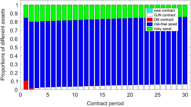
Figure 11 The composition of the optimal portfolio for different terms using the value function and weighting function defined in Tversky & Kahneman (Reference Tversky and Kahneman1992). r f =0.04, μ=0.1 and σ=0.2.
As the Figure 11 shows, GJN contract is an attractive contract under the EUT. Especially, with the increase of the investment horizon, the proportion of the GJN contract is increasing gradually while the proportion of risky asset is decreasing. As the replicating portfolio of the GJN contract consists of the more risky asset (less risk-free asset) for long-horizon contracts than shortFootnote 10 , the optimal portfolio in Figure 11 seems to provide an approximated strategy to the Merton’s solution.
6 Conclusion
In this paper, we examine a new pension contract in the accumulation phase of a pension scheme. This new contract occupies the characteristics of guarantees and bonuses but has a transparent structure and clear profit distribution rule. Under CPT, the contract gives higher utility than the contract introduced in Guilléen et al. (Reference Guilléen, Jørgensen and Nielsen2006) and the contract studied by Døskeland & Nordahl (2008 Reference Døskeland and Nordahlb ).
The result shows that shielding customers from poor stock market returns is attractive to the customer. By the application of financial engineering techniques in pricing and risk management, the insurer can manage the additional risk which it faces in issuing such guarantees. In addition, we show that with the increase of policyholder’s investment horizon, the proportion of the risky asset in the optimal portfolio grows larger while the proportion of the risk-free asset decreases. This result conforms to traditional pension investment advice that young people should invest more money in the risky asset while old people should reduce their exposure to risky assets.
There are much more we can investigate to continue our research. For example, as we only find the best buy-and-hold strategy among some different sub-optimal dynamic strategies. Hence, finding the product which matches the dynamic optimal investment strategy is an interesting area for future research.
Acknowledgements
The author thanks an anonymous referee for kindly reviewing the paper. He gratefully appreciates the supervising from Catherine Donnelly, Andrew Cairns and Torsten Kleinow. Support for this research from the Actuarial Research Centre of the Institute and Faculty of Actuaries is gratefully acknowledged.


