1. INTRODUCTION
Attitude estimation using Micro Electro-Mechanical Systems (MEMS)-based inertial sensors is an essential task for an Unmanned Aerial Vehicle (UAV) for flight control. Attitude estimation can be achieved by fusing data obtained from Inertial Measurement Units (IMUs) composed of a three-axis gyroscope, a three-axis accelerometer and a three-axis magnetometer (Lou et al., Reference Lou, Neal, Labrosse and Cao2011; Edwan et al., Reference Edwan, Zhang, Zhou and Loffeld2011; Hoflinger et al., Reference Hoflinger, Muller, Zhang, Reindl and Burgard2013). However, the use of inertial/magnetic sensor modules to estimate attitude has some significant challenges. Since the gyroscope has high drift and noise, it is inaccurate to directly integrate the angular velocity of the gyroscope. Therefore, as an auxiliary sensor for correcting the drift, an accelerometer and a magnetometer are employed, but the accelerometer is sensitive under dynamic motion conditions. However, magnetometers are easily hindered by the electrical noise of electrical devices or appliances made of ferrous materials (Bachmann et al., Reference Bachmann, Yun and Brumfield2007). For micro-UAV, attitude estimation can be realised using only accelerometer and gyroscope data (Hyde et al., Reference Hyde, Ketteringham, Neild and Jones2008; Zhang et al., Reference Zhang, Xian, Zhao and Zhang2015).
Generally, the attitude estimation of data from an IMU can be implemented by using an algorithm based on a Kalman filter, such as an Extended Kalman Filter (EKF) or Complementary Kalman Filter (Hide et al., Reference Hide, Moore and Smith2003; Marina et al., Reference Marina, Pereda, Giron-Sierra and Espinosa2012; Wang, Reference Wang2013; Markley and Sedlak, Reference Markley and Sedlak2008; Xue et al., Reference Xue, Leung, Wang, Liu and Wu2015; Ligorio and Sabatini, Reference Ligorio and Sabatini2015; Chang et al., Reference Chang, Chan and Jin2016). These Kalman filter-based algorithms are prone to divergence and have several problems both in theory and in practice, due to computation of noise model and covariance (Nowicki et al., Reference Nowicki, Wietrzykowski and Skrzypczynski2015).
Attitude estimation can also be solved by using iterative methods, such as particle filtering, (Carmi and Oshman, Reference Carmi and Oshman2012; Cappello et al., Reference Cappello, Sabatini, Ramasamy and Marino2015), Mahony filtering (Grip et al., Reference Grip, Fossen, Johansen and Saberi2012), Gradient Descent Algorithm (GDA) (Madgwick et al., Reference Madgwick, Harrison and Vaidyanathan2011); Cheguini and Ruiz, Reference Cheguini and Ruiz2012) and Gauss-Newton Algorithm (GNA) (Liu et al., Reference Liu, Li, Wang and Liu2014); (Jategaonkar, Reference Jategaonkar2015; Barrau and Bonnabel, Reference Barrau and Bonnabel2013). However, these algorithms are expensive in computational terms and unsuitable for a micro-UAV with small scale embedded processors, even if most are effective.
Though the EKF is considered to be the standard framework for solving attitude estimation problems in navigation, in practice a much simpler Complementary Filter (CF) is often applied in micro-UAV with limited resources (Euston et al., Reference Euston, Coote, Mahony and Kim2008; Mahony et al., Reference Mahony, Tarek and Jean-Michel2008; Tseng et al., Reference Tseng, Li, Sheng, Hsu and Chen2011; Chang et al., Reference Chang, Mu and Shen2011; Wu et al., Reference Wu, Zhou, Chen, Fourati and Li2016). It contains a simple calculation process, but the performance is poor (Nowicki et al., Reference Nowicki, Wietrzykowski and Skrzypczynski2015). This limitation of complementary filters can be overcome by using adaptive-gain. Calusdian et al., (Reference Calusdian, Yun and Bachmann2011) presented a complementary filtering algorithm for attitude estimation which utilises a single gain that can be self-adjusted to achieve a satisfactory performance when tracking two or more different types of motion. Tian et al., (Reference Tian, Wei and Tan2013) presented an analytically derived method for an adaptive-gain complementary filter based on the convergence rate from the Gauss-Newton optimisation algorithm. Widodo et al. (Reference Widodo, Edayoshi and Wada2014) presented a design of an adaptive mechanism to adjust gain using a fuzzy logic controller, and dynamic acceleration and change in dynamic acceleration can be used as inputs for the controller.
In this paper, a novel complementary filter algorithm with a self-adjusted gain is proposed. The proposed algorithm combines translation attitude estimation from the accelerometer output with rotation attitude estimation from the gyroscope output, which utilises a gain that can be self-adjusted to reach a good performance.
There are two main contributions of this paper: firstly, the attitude calculated by the accelerometer data is transformed to a solution of a linearly discrete dynamic system to reduce the computing time. Secondly, a novel complementary filter structure is proposed.
This paper is organised as follows. Section 2 introduces attitude estimation calculated using the measurement data from accelerometer and gyroscope. In Section 3, the main structure of the proposed algorithm is explained. Simulation and experimental results are shown in Section 4 to evaluate the performance compared with conventional algorithms. Finally, Section 5 presents conclusions.
2. ATTITUDE ESTIMATION
The attitude of an UAV can be measured through the attachment of an IMU module. In this paper, a IMU consisting of a tri-axis accelerometer and a tri-axis gyroscope is adopted to estimate the attitude. To represent the rotation between different coordinate systems (body coordinate system and Earth coordinate system), there are three mathematical rotation representations: Euler angles, rotation matrix and quaternion. In this paper, the quaternion representation is used because of its high computational efficiency, which is shown as follows:
 $${\bf q}=\left[{\matrix{{q_0 } & {q_1 } & {q_2 } & {q_3 }}}\right]^{\rm T} $$
where q represents the rotation of three-dimensional space, which consists of four components; and  $q_{0}^{2} +q_{1}^{2} +q_{2}^{2} +q_{3}^{2} =1$.
2.1. Attitude from gyroscope data
The angular velocity measured by gyroscope is represented by the following equation in the body coordinate system b:
 $${\bf M}_g^b =\lpar {\omega_x \comma \; \omega_y \comma \; \omega_z} \rpar ^{\rm T} $$
where  ${\bf M}_{g}^{b}$ is the angular velocity measured by the gyroscope in the body coordinate system, which consists of three components, and
  $\omega _{x} \comma \; \omega _{y} \comma \; \omega _{z}$ are the measurements of gyroscopes in the x-axis, y-axis and z-axis, respectively.
The derivative of attitude angle provided by the gyroscope in the body frame relative to the Earth frame can be calculated as shown in the following equation using the quaternion representation.
 $${\dot {\bf q}}_{g\comma t} = \displaystyle{1 \over 2}{\bf R}_g \otimes {\bf q}_{g\comma t - 1} $$
where  ${\dot{\bf q}}_{g\comma t}$ is the derivative of attitude angle provided by the gyroscope and
  ${\bf q}_{g\comma t-1}$ is the quaternion representation of the angle estimated by the gyroscope at time t − 1. Rg is a 4 × 4 skew-symmetric matrix, which can be represented as:
 $${\bf R}_g =\left[{\matrix{ 0 & {-\omega_x } & {-\omega_y } & {-\omega_z } \cr {\omega_x } & 0 & {\omega_z } & {-\omega_y }\cr {\omega_y } & {-\omega_z } & 0 & {\omega_x }\cr {\omega_z } & {\omega_y } & {-\omega_x } & 0\cr }}\right]$$
2.2. Attitude from accelerometer data
The measurement provided by accelerometer in the Earth coordinate system (North-East-Down) is shown in Equation (5):
 $$\left\{{\matrix{{\bf M}_a^b =\lpar {a_x \comma \; a_y \comma \; a_z } \rpar^{\rm T} \hfill \cr {\bf M}_a^b ={\bf C}_e^b {\bf M}_a^e \hfill \cr {\bf M}_a^e =\lpar {0\comma \; 0\comma \; 1} \rpar^{\rm T} \hfill \cr}}\right. $$
where  ${\bf M}_{a}^{b}$ and
  ${\bf M}_{a}^{e}$ are the measurement vectors of the accelerometer in the body coordinate system b and Earth coordinate system e, respectively and a x, a y, a z are the measurements of the accelerometers in the x-axis, y-axis and z-axis, respectively.
  ${\bf C}_{e}^{b}$ is the Direction Cosine Matrix (DCM) from the Earth coordinate system to the body coordinate system.
The matrix  ${\bf C}_{e}^{b}$ can be expressed as:
 $${\bf C}_e^b =\left[{\matrix{{q_0^2 +q_1^2 -q_2^2 -q_3^2 } & {2\lpar {q_1 q_2 +q_0 q_3 } \rpar } & {2\lpar {q_1 q_3 -q_0 q_2 } \rpar } \cr {2\lpar {q_1 q_2 -q_0 q_3 } \rpar } & {q_0^2 -q_1^2 +q_2^2 -q_3^2} & {2\lpar {q_0 q_1 +q_2 q_3 } \rpar } \cr {2\lpar {q_1 q_3 +q_0 q_2 } \rpar } & {2\lpar {q_2 q_3 -q_0 q_1 } \rpar } & {q_0^2 -q_1^2 -q_2^2 +q_3^2}\cr}}\right]$$
Hence, Equation (5) can be expressed as:
 $${\bf M}_a^b =\left[{\matrix{{2\lpar {q_1 q_3 -q_0 q_2 } \rpar } \cr {2\lpar {q_0 q_1 +q_2 q_3 } \rpar } \cr {q_0^2 -q_1^2 -q_2^2 +q_3^2 } \cr}}\right]=\left[{\matrix{ {-q_2 } & {q_3 } & {-q_0 } & {q_1 } \cr {q_1 } & {q_0 } & {q_3 } & {q_2 } \cr {q_0 } & {-q_1 } & {-q_2 } & {q_3 } \cr}}\right]\left[{\matrix{{q_0 } \cr {q_1 } \cr {q_2 } \cr {q_3 } \cr }} \right]={\bf Pq}_a $$
where qa is the quaternion representation of the angle estimated by the accelerometer and P can be expressed as:
 $${\bf P}=\left[{\matrix{{-q_2 } & {q_3 } & {-q_0 } & {q_1 } \cr {q_1 } & {q_0 } & {q_3 } & {q_2 } \cr {q_0 } & {-q_1 } & {-q_2 } & {q_3} \cr }}\right]$$
Therefore, Equation (7) can be transformed into the following equation:
 $$\eqalign{{\bf q}_a & = {\bf P}^{\prime}{\bf M}_a^b \cr & \Rightarrow \left[{\matrix{{q_0 } \cr {q_1 } \cr {q_2 } \cr {q_3} }}\right]=\left[{\matrix{{-q_2 } & {q_1 } & {q_0 } \cr {q_3 } & {q_0 } & {-q_1 } \cr {-q_0 } & {q_3 } & {-q_2 } \cr {q_1 } & {q_2 } & {q_3} \cr}}\right]\left[{\matrix{{a_x } \cr {a_y } \cr {a_z }\cr }}\right]= \left[{\matrix{{-a_x q_2 +a_y q_1 +a_z q_0} \cr {a_x q_3 +a_y q_0 -a_z q_1 } \cr {-a_x q_0 +a_y q_3 -a_z q_2 } \cr {a_x q_1 +a_y q_2 +a_z q_3} \cr}}\right]\cr & \Rightarrow \left[{\matrix{{q_0 } \cr {q_1 } \cr {q_2 } \cr {q_3 } \cr}}\right]=\left[{\matrix{{a_z } & {a_y } & {-a_x } & 0 \cr {a_y } & {-a_z } & 0 & {a_x } \cr {-a_x } & 0 & {-a_z } & {a_y } \cr 0 & {a_x } & {a_y } & {a_z } \cr}} \right]\left[{\matrix{{q_0 } \cr {q_1 } \cr {q_2 } \cr {q_3 } \cr}}\right]={\bf R}_a {\bf q}_a}$$
One can observe that:
 $${\bf R}_a^2 =\left[{\matrix{{a_z } & {a_y } & {-a_x } & 0 \cr {a_y } & {-a_z } & 0 & {a_x } \cr {-a_x } & 0 & {-a_z } & {a_y } \cr 0 & {a_x } & {a_y } & {a_z } \cr }}\right]^2={\bf I}_{4\times 4} $$
Equation (9) can be denoted as the following equation:
 $${\bf q}_{a\comma t} = {\bf R}_a {\bf q}_{a\comma t-1} $$
where qa,t−1 is the quaternion provided by accelerometer measurement at time t − 1.
A continuous system and a linear discrete constant dynamic system can be represented as Equation (12).
 $$\left\{\matrix{{\dot {\bf x}}\lpar t\rpar = {\bf Ax} + {\bf Bu}\lpar t\rpar \hfill \cr {\bf x}\lpar k + 1\rpar = {\bf Gx}\lpar k\rpar + {\bf Hu}\lpar k\rpar }\right. $$
where u is the system input and x is the status of the system, A and G are the system matrices, B and H are the input matrices.
According to modern control theory (Liu and Tang, Reference Liu and Tang2006), we can derive the following equation:
 $${\bf G} = \exp ^{{\bf A} \tau } $$
Therefore, Equation (11) can be seen as a linear discrete constant dynamic system with input u(k) = 0.
Then,
 $${\bf R}_a = {\bf G} = \exp ^{A\tau } $$
The approximate solution can be obtained as:
 $${\bf R}_a ={\bf I}_{4\times 4} +{\bf A}\tau \Rightarrow {\bf A}=\displaystyle{{{\bf R}_a -{\bf I}_{4\times 4}}\over{\tau}} $$
Using the Taylor series expansion method for Equation (14):
 $$\exp ^{{\bf A}\tau }={\bf I}_{4\times 4} +{\bf A}\tau +\displaystyle{{{\bf A}^2\tau ^2}\over{2!}}+\cdots +\displaystyle{{{\bf A}^n\tau ^n}\over{n!}} $$
where:
 $$\eqalign{{\bf A}^{\rm 2} & =\left({\displaystyle{{{\bf R}_a -{\bf I}_{4\times 4} }\over{\tau }}} \right)^2 =\displaystyle{{{\bf R}_a^2 -2{\bf R}_a +{\bf I}_{4\times 4} }\over{\tau ^2}} \cr &=-\displaystyle{{2}\over{\tau }}\displaystyle{{{\bf R}_a -{\bf I}_{4\times 4}}\over{\tau}}=-\displaystyle{{2}\over{\tau }}{\bf A} \cr {\bf A}^3&=\left({-\displaystyle{{2}\over{\tau}}} \right)^2{\bf A}}$$
Therefore, Equation (16) becomes:
 $$\eqalign{\exp^{{\bf A}\tau} &={\bf I}_{4\times 4} +{\bf A}\tau +\displaystyle{{-2}\over{2!}}{\bf A}\tau +\displaystyle{{\lpar {-2} \rpar ^2}\over{3!}}{\bf A}\tau +\cdots +\displaystyle{{\lpar {-2} \rpar ^{n-1}}\over{n!}}{\bf A}\tau \cr & ={\bf I}_{4\times 4} +{\bf A}\tau \left({1+\displaystyle{{-2}\over{2!}}+\displaystyle{{\lpar {-2} \rpar^2}\over{3!}}+\cdots +\displaystyle{{\lpar {-2}\rpar^{n-1}}\over{n!}}} \right)} $$
Define:
 $$\Pi = 1 + \displaystyle{{ - 2} \over {2!}} + \displaystyle{{{\lpar - 2\rpar }^2} \over {3!}} + \cdots + \displaystyle{{{\lpar - 2\rpar }^{n - 1}} \over {n!}} $$
 $$- 2\Pi = \lpar - 2\rpar + \displaystyle{{{\lpar - 2\rpar }^2} \over {2!}} + \displaystyle{{{\lpar - 2\rpar }^3} \over {3!}} + \cdots + \displaystyle{{{\lpar - 2\rpar }^n} \over {n!}} $$
Hence:
 $$\eqalign{1-2 \Pi &= 1+\lpar {-2} \rpar +\displaystyle{{\lpar {-2} \rpar ^2}\over{2!}}+\displaystyle{{\lpar {-2} \rpar ^3}\over{3!}}+\cdots +\displaystyle{{\lpar {-2} \rpar ^n}\over{n!}} \cr &=\exp ^{-2}} $$
Equation (17) becomes:
 $$\exp ^{{\bf A}\tau}={\bf I}_{4\times 4} +\displaystyle{{1-\exp ^{-2}}\over{2}}\lpar {{\bf R}_a -{\bf I}_{4\times 4} } \rpar $$
Equation (11) can be transformed into the following equation:
 $${\bf q}_{a\comma t} =\exp^{{\bf A}\tau }{\bf q}_{a\comma t-1} =\left({\displaystyle{{1+\exp^{-2}}\over{2}}{\bf I}_{4\times 4} +\displaystyle{{1-\exp^{-2}}\over{2}}{\bf R}_a}\right){\bf q}_{a\comma t-1}$$
 $$\Delta {\bf q}_{a\comma t} =\displaystyle{{1-\exp ^{-2}}\over{2}}\lpar {{\bf R}_a -{\bf I}_{4\times 4} } \rpar {\bf q}_{a\comma t-1} $$
3. FAST ADAPTIVE COMPLEMENTARY FILTER (FACF)
A Complementary Filter (CF) is designed for two noise sources with complementary spectral characteristics. The idea is to pass the accelerometer signals through a low-pass filter and the gyroscope signals through a high-pass filter, then combine them to obtain the final results. This is particularly well suited to fusing data for attitude estimation of a UAV, because the relations between attitude angular rate and attitude in different dynamical modes of a quad-rotor include high and low frequency. A low-pass filter is used in translational motion and a high-pass filter is used in rotation motion.
The standardised first order complementary filter estimated attitude is given by Equation (24):
 $${\bf q}_{CF\comma t} =k\; {\bf q}_{g\comma t} +\lpar {1-k} \rpar {\bf q}_{a\comma t}\comma \; \quad k\in \lpar {0\comma \; 1} \rpar $$
where qg,t and qa,t are the angle calculated by gyroscope data and the angle calculated by accelerometer data, respectively. k is the gain of the CF and qCF,t is the estimated attitude from the CF.
The estimated attitude can be described by Equation (25):
 $${\bf q}_{CF\comma t} ={\bf q}_{CF\comma t-1} +\dot{{\bf q}}_{CF\comma t} \Delta t $$
whereΔ t is the sampling time.
Hence, Equation (25) can be expressed as Equation (26) using Equations (3), (22) and (24):
 $$\eqalign{{\bf q}_{CF\comma t} & ={\bf q}_{CF\comma t-1} +\lsqb {k\; \dot{{\bf q}}}_{g\comma t} +\lpar {1-k} \rpar \dot{{\bf q}}_{a\comma t}\rsqb \Delta t \cr &=\lsqb {k\; {\bf q}_{g\comma t-1} +\lpar {1-k} \rpar {\bf q}_{a\comma t-1} } \rsqb \; +\displaystyle{{k}\over{2}}{\bf R}_g {\bf q}_{g\comma t-1}\Delta t+\lpar {1-k} \rpar \Delta {\bf q}_{a\comma t} \cr & =\left[{k\left({{\bf I}+\displaystyle{{1}\over{2}}{\bf R}_g \Delta t}\right)\ \lpar {1-k} \rpar \left[{\displaystyle{{\lpar {1-\exp^{-2}} \rpar {\bf R}_a }\over{2}}+\displaystyle{{\lpar {1+\exp^{-2}} \rpar {\bf I}_{4\times 4} }\over{2}}}\right]}\right]\lsqb {{\bf q}_{g\comma t-1} \; \; {\bf q}_{a\comma t-1} } \rsqb ^T}$$
The block diagram of the FACF is shown in Figure 1. Data retrieved from the accelerometer is filtered through a low pass filter. Then the attitude angle can be calculated from the accelerometer data. Data provided by the gyroscope is adjusted through the gyroscope bias and then the attitude angle can be calculated from the gyroscope data. Finally, the angle from the accelerometer data and the angle from the gyroscope data are fused by the FACF with an adaptive weight coefficient.
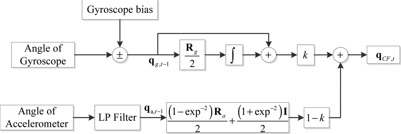
Figure 1. The block diagram of the proposed algorithm.
The accuracy of filter output is determined by the value of the feedback gain k. Because of the flexible and fast manoeuvring of a UAV, the value of gain k should be designed to be adjustable. Generally speaking, a larger value is preferred when the UAV is in the state of rotational motion. Conversely, a smaller value is preferred when the UAV is in the state of translational motion. The value range of gain k is set as: [0·6, 0·95] based on experience and tests, and the initial value is 0·8.
4. SIMULATION AND EXPERIMENTAL RESULTS
4.1. Experiment setup
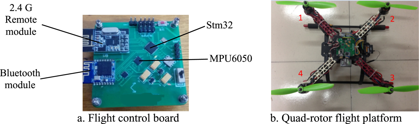
To verify the proposed algorithm, a platform as shown in Figure 2 was developed with programming implemented using the C language. The developed IMU sensors contain a tri-axis gyroscope and a tri-axis accelerometer (MPU6050). The chip also has an embedded processor (stm32) for computation and Bluetooth module to transmit data. All sensor signals are sampled at 50 Hz and interfaced to a ground station via the Bluetooth module which is convenient for data analysis. The basic specification of the quad-rotor in the experiment is shown in Table 1.

Figure 2. Experimental platform.
Table 1. The basic specification of the quad-rotor.
4.2. Experiment results and discussion
4.2.1 Test 1: Sensor calibration
Due to the characteristics of its material, the accuracy and stability of the gyro's output are mainly affected by the resonant frequency of the gyro. The relationship between resonant frequency and temperature can be expressed in the following equation:
 $${}^b\omega \lpar T\rpar ={ }^b\omega \lpar {T_0 } \rpar \lsqb {1-1/2k_{ET} \Delta T} \rsqb $$
where k ET is the variation coefficient of the gyro whose value is usually in the order of 10−6. Δ T is the variation in temperature compared to the room temperature and ω is the measurement provided by the gyroscope.
Temperature is the most important effect on the physical characteristics of the gyroscope. The slowly time-varying bias can be compensated by modelling the curve of temperature and bias. This is done by placing the gyro in the refrigerator to keep it at 0°C. Then it is placed in an environment with a room temperature of 30°C. The outputs of the gyro are recorded and fitted; the fitted equation and curve are shown in Equation (20) and Figure 3.
Figure 3. The fitted curves of gyroscope outputs.
 $$\eqalign{g_{out}^x &=-1\cdot4\ast \exp ^{\lpar {-\lpar {\lpar {t-8\cdot3} \rpar /50\cdot4} \rpar^2} \rpar } \cr g_{out}^y &=0\cdot8\ast \exp ^{\lpar {-\lpar {\lpar {t-26\cdot2} \rpar /30\cdot3} \rpar^2} \rpar } \cr g_{out}^z &=7\cdot52\exp -07\ast t^4-2\cdot05\exp -05\ast t^3-0\cdot000275\ast t^2+0\cdot023\ast t-2\cdot95} $$
where t is the temperature of the gyroscope, and  $g_{out}^{x} \comma \; g_{out}^{y}\comma \; g_{out}^{z}$ are the output of the gyroscope in x-axis, y-axis and z-axis after temperature compensation, respectively.
Because of the installation error and the characteristics of the accelerometer, the accuracy and stability of the gyro's output are poor. Therefore, calibration of the data provided from the gyro is needed. In order to reduce the installation error, an offset should be subtracted from the output of the accelerometer by taking the average value of the first 400 outputs of the accelerometer in its initial state. In order to reduce the error due to the characteristics of the accelerometer, the moving average filtering expressed in Equation (29) is adopted.
 $${}^b{a}_{out}\lsqb i\rsqb = \displaystyle{1 \over n}\sum\limits_{j = 0}^{n - 1} {{}^{b}{\tilde a}_{out}\lsqb i + j\rsqb } $$
where  ${ }^{b}a_{out} \; \hbox{and}{ }^{b}\; \tilde {a}_{out}$ are the accelerometer measurements in the body coordinate system before and after filtering respectively, and n is the sampling spot number.
The adjusted output of the accelerometer is shown in Figure 4.
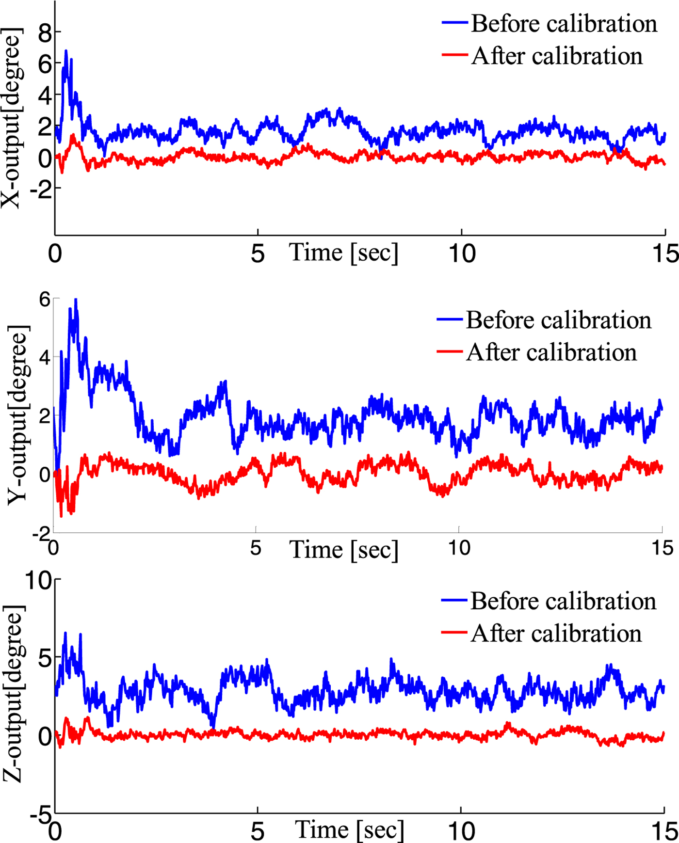
Figure 4. Results of accelerometer calibration.
4.2.2. Test 2: Hovering
In order to test the accuracy and reliability of the proposed algorithm, an open source platform (Pixhawk flight control system) was chosen to test it. The self-stabilisation mode was selected to fly indoors. In this mode, only the attitude control loop is implemented. Therefore, the attitude of the UAV can maintain a stable state, but the position will drift. In this experiment, the UAV is in a translational state and the rotation motion is very small. Therefore the reliability of accelerometers is relatively high and the weight given to the accelerometer in the algorithm is increasing and the value of k is lowered from 0·8 to about 0·6. The responses are depicted in Figure 5 and the specific performance indices are shown in Table 2. Results show that FACF has a slightly worse performance in accuracy compared with EKF. This is because the angular velocity of the UAV is very small (about 2°/s) in this situation and the proposed algorithm takes a few seconds (about 4 seconds) to adjust the gain (k = k − 0·05).
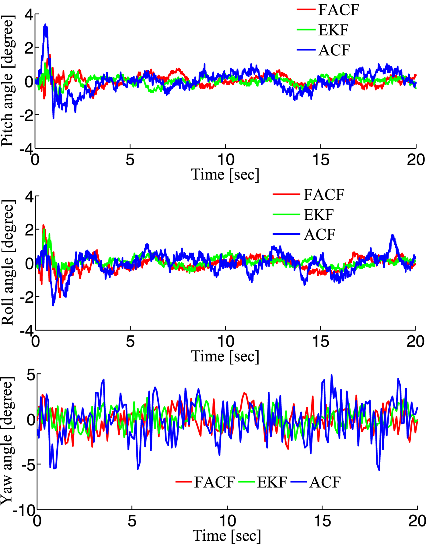
Figure 5. Responses with three algorithms in Test 2.
Table 2. The performance indices of three algorithms during hovering.

The reason why the accuracy of the CF is relatively poor is that the gain is fixed. In order to improve the accuracy of the algorithm, the gain should be designed to be adjustable with time according to the different motion states. In Calusdian et al., (Reference Calusdian, Yun and Bachmann2011), the method proposed only adjusts the gain with three fixed numbers corresponding to the acceleration. The accuracy of this algorithm has not been greatly improved. Therefore, FACF has a better performance compared with the Adaptive-gain Complementary Filter (ACF) proposed by Calusdian et al. (Reference Calusdian, Yun and Bachmann2011).
4.2.3. Test 3: Large angle reference tracking in coupling condition
In this simulation the attitudes are required to track the sinusoidal signal reference at different times. The amplitude of the signal reference in attitude angle is from –10o to 10o. The responses are depicted in Figure 6 and the specific performance indices (Max error and Root Mean Square Error (RMSE)) are shown in Table 3. In this situation the UAV is in a rotation state and the translational motion is very small. Therefore the reliability of the gyroscope is relatively high and the weight given to the gyroscope in the algorithm is increasing and the value of k immediately increases from 0·8 to 0·95 (k = k + 0·1). Results show that FACF has a similar performance in accuracy compared with EKF, but a better performance compared with ACF.
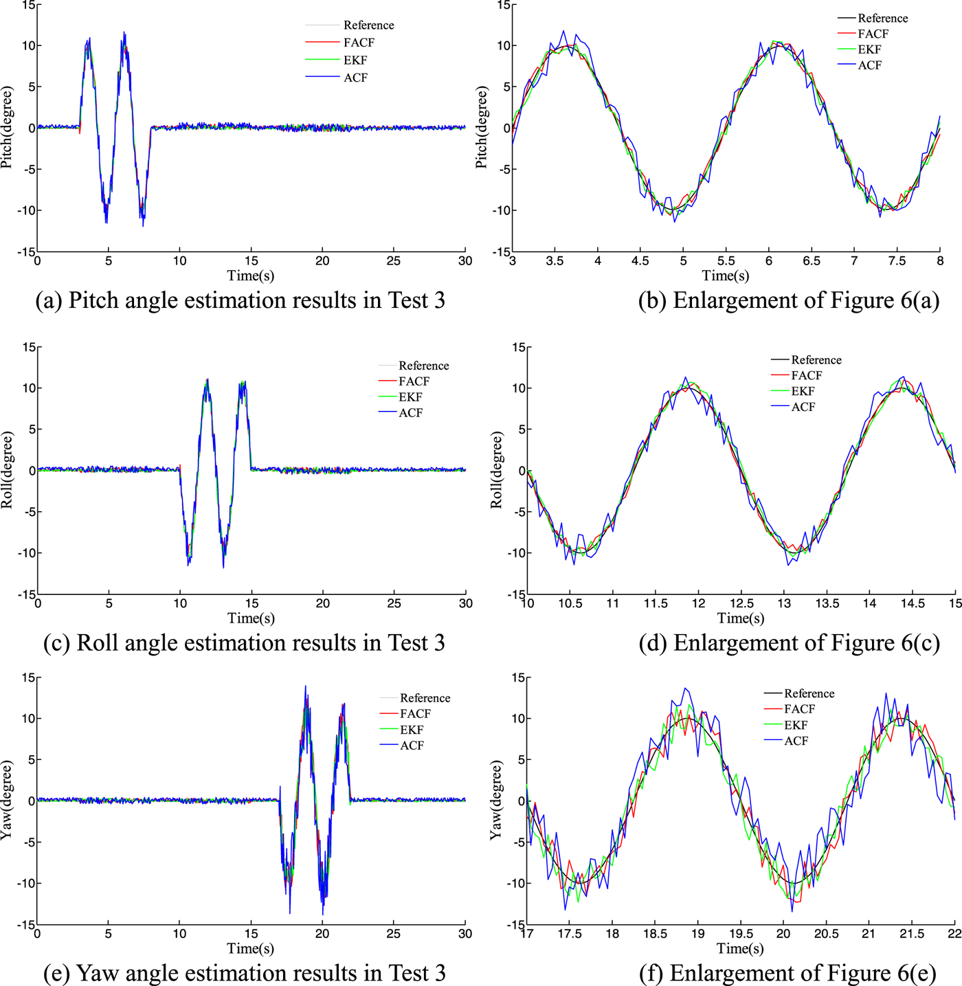
Figure 6. Responses with three algorithms in Test 3.
Table 3. The performance indices of three algorithms during large angle tracking.
4.2.4. Test 4: Computing time
The aim of this test is to compare the run time of the three algorithms. A semi-physical simulation was adopted in this test. The IMU data was obtained through the serial port and the three algorithms then ran 1,000 times and output the time consumption.
The times required to perform 1,000 repetitions of FACF, EKF (an algorithm adopted by the open-source platform Pixhawk) and ACF are shown in Table 4. The result shows that the computing time of FACF is less than EKF and about the same as ACF. This is because the EKF requires a massive amount of matrix operations. Though FACF and ACF have the same time consumption, the accuracy of FACF is better than ACF. Therefore, the proposed FACF finds a balance between accuracy and time consumption.
Table 4. The time required to perform 1,000 repetitions of three algorithms (seconds).

4.3. Discussion
In engineering applications, a good algorithm should find a balance between time consumption and accuracy. The advantages of the CF are that it is simple for computation and has the property of a small amount of calculations. Therefore, the primary objective of an algorithm based on a complementary filter is to improve the performance in accuracy. Due to the structural problems of a complementary filter, an algorithm based on a complementary filter can be considered as a good algorithm if the performance in accuracy is similar to EKF.
As mentioned above, results show that when the UAV is hovering or makes a rotational motion, the value of gain will be adjusted according to the scale value of angular velocity. Simulation and experimental results show that the accuracy performance of the proposed algorithm is as good as EKF. The performance of the proposed algorithm in time consumption ranks ahead of EKF and is as good as ACF. Therefore, the proposed algorithm successfully finds a balance between time consumption and accuracy.
5. CONCLUSION
A fast adaptive-gain complementary filter is proposed to estimate the attitude of a UAV using IMU sensors (gyroscope and accelerometer). In order to improve the accuracy of a complementary filter, a novel structure of complementary filter is proposed. Moreover, a novel attitude estimation algorithm calculated from accelerometer data is proposed to reduce the computing time. The experimental results show the validity and accuracy of the proposed algorithm, which has advantages of strong robustness and lower time consumption.
FINANCIAL SUPPORT
This research received no specific grant from any funding agency, commercial or not-for-profit sectors.