I. Introduction
Whenever consumers have access to perfect information, the Bertrand model indicates that the equilibrium price of goods and services equals its marginal cost. In practice, however, the law of one price is the exception rather than the rule. In fact, most markets are characterized by substantial price dispersion. This is particularly true for experience goods, for which quality is known only after purchase and consumption. However, it is costly to acquire information for consumers. The pioneering research by Akerlof (Reference Akerlof1970) and Nelson (Reference Nelson1970) established that information asymmetries that pertain to the quality of a product might influence markets in a detrimental way.
Brands (Montgomery and Wernerfelt, Reference Montgomery and Wernerfelt1992), advertising (Ackerberg, Reference Ackerberg2003), quality labeling (Jin and Leslie, Reference Jin and Leslie2003), and expert endorsement (Salop, Reference Salop1976) all constitute transmission channels that provide consumers with information about a product's quality. Although there are experts in a variety of domains—art, economics, weather forecasting, sport, gastronomy, cars, and electronics—it is extremely difficult to assess their influence and the quality of their opinions on products. Reinstein and Snyder (Reference Reinstein and Snyder2005) concluded that movie reviews do not affect a film's box office earnings. Sorensen and Rasmunssen (Reference Sorensen and Rasmussen2004) demonstrated that book reviews, whether favorable or unfavorable, boosted sales, thereby confirming the old adage “there is no such thing as bad publicity.” Indeed, empirical studies face a major methodological problem: high-quality products obtain high scores because they are, in fact, of high quality. Thus, it becomes difficult to determine the extent to which expert endorsements stimulate demand. Recent papers by Hodgson (Reference Hodgson2008, Reference Hodgson2009) question the consistency of expert wine judges in a wine competition setting and demonstrate that wine experts make mistakes. Ashton (Reference Ashton2011) and Lecocq and Visser (Reference Lecocq and Visser2006) point out, however, that judgment errors can be reduced by pooling the opinions of several experts.
Bordeaux wine represents an experience good that requires a great deal of expertise in order to determine each wine's final quality and, hence, its price. This paper seeks to establish whether the experts, including the most renowned, Robert Parker, provide pertinent information for consumers and whether their scores influence wine prices.
For Ashenfelter (Reference Ashenfelter1989), the fallibility of Parker's judgment allows buyers to profit from his errors of judgment when wines are sold at auction. According to Ashenfelter (Reference Ashenfelter2008), a wine's age, the average temperature from April to September, the rainfall in August and September and then from October to March, and the vintage are the main factors behind price variations. Ashenfelter and Jones (Reference Ashenfelter and Jones2013) show that expert scores on Bordeaux wine do not provide useful information in poor years and correlate only with market prices, at best, in good years. Experts tend to disregard key data such as weather conditions during the growing season, which crucially determine the wine's quality. As there is detailed information about local weather conditions, in particular, available privately to each individual château (Di Vittorio and Ginsburgh, Reference Di Vittorio and Ginsburgh1994), the experts merely transmit publicly available information to the consumer. Ginsburgh et al. (Reference Ginsburgh, Monzak and Monzak1992) apply the hedonic pricing model to a sample of 102 Médoc wines in order to show that expert ratings do not provide a better explanation for price than climate conditions, the 1855 classification, terroir, or production technique. Sixty-six percent of price variations could be explained by weather conditions or differences in vineyard practices. This percentage rose to 85% when the 1855 classification was taken into account. Di Vittorio and Ginsburgh (Reference Di Vittorio and Ginsburgh1994) come to the same conclusion. A hedonic function, calculated on the basis of the auction prices of 58 Médoc crus classés, indicate that the 1855 classification plays a greater role in explaining a wine's price than any alternative rating system drawn up by experts.
For Jones and Storchmann (Reference Jones and Storchmann2001), Parker's scores influence prices in a differentiated fashion. Their analysis suggests that a rise of one point may cause price increases between 4% and 10%, with an average increase of 7%. This result, obtained from prices for 21 prestigious Bordeaux wines, indicates that the sensitivity of a wine's price relative to Parker's scores is greater for wines made from Cabernet-Sauvignon than for those made from Merlot. Hilger et al. (Reference Hilger, Rafert and Villas-Boas2011), adopting a more experimental approach, also showed the impact of expert ratings. They analyzed wine sales in a supermarket by choosing a random sample of 150 wines from 476 rated wines and displaying each wine's score on supermarket shelves. Sales of the selected wines increased by an average of 25%, and sales of those with the best scores increased more quickly than those with lower scores. This led to the conclusion that the advertising surrounding expert endorsement produces a positive effect on global demand as it reduces information asymmetry. Storchmann et al. (Reference Storchmann, Mitterling and Lee2012) argued that expert opinion has a negative effect on the price dispersion of American wines evaluated by the Wine Spectator between 1984 and 2008. The authors show that expert opinion distorts the relationship between quality and price, especially in the case of poor-quality wines. Roma et al. (Reference Roma, Di Martino and Perrone2013) constructed a hedonic price model to determine the variables influencing the prices in a sample of Sicilian wines. They concluded that price depends on traditional objective variables and sensorial variables as well as on the ratings published in specialized reviews. Using five years of data on expert opinions published in six Swedish periodicals, Friberg and Grönqvist (Reference Friberg and Grönqvist2012) showed how a positive review induced an increase in demand of 6% the week after publication. This positive effect then declined but was still significant 20 weeks later. A neutral expert opinion led to a small increase in demand, whereas a negative opinion had no effect.
The debate about the impact of expert opinion on price is even more complicated for Bordeaux wines. Bordeaux crus classés can be sold en primeur in the futures market six months after harvesting and are delivered to the purchaser only two or three years later. This creates a great deal of uncertainty concerning the wine's ultimate quality. It is the expert's role to ascertain this ultimate quality, which, consequently, influences the sale prices of primeur wines. Ali and Nauges (Reference Ali and Nauges2007), using a sample of 108 châteaux for vintages from 1994 to 1998, showed that the price en primeur is determined chiefly by reputation. Parker's scorings have a significant but marginal effect—an increase of one point triggered a rise in price of 1.01%.
Simply put, the role of experts in influencing the price of any wine remains uncertain and differs from one study to another. Wine is not a homogeneous product but varies according to a set of characteristics. Some of these characteristics—color or grading, for example—are easy to measure inexpensively. Others, such as sensorial or taste characteristics, are difficult to measure before consumption. Expert opinions are purported to summarize quality characteristics of wine. These opinions may convey less information than a complete description of characteristics. In addition, these opinions might be imperfect because they fail to capture, for example, the quality experienced by consumers. This imperfection can have implications for prices and consumer welfare.
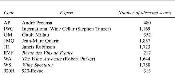
The present research aims to investigate the question of the impact of expert opinion on fixing the retail price of wine. It is based on exhaustive data concerning the scores attributed to different wines by a broad panel of nineFootnote 1 wine experts from three different countries over 11 years (2000 to 2010). Our main objective is to reduce the systematic econometric bias that is bound up with expert opinion and to test the impact on prices of a consensus or divergence among experts. Evidence of this bias has been revealed by Lecocq and Visser (Reference Lecocq and Visser2006) as well as Oczkowski (Reference Oczkowoski2001).
As a first attempt to correct the measurement error bias, we aggregate a solid body of information from those nine experts to reduce the risk of error from any one expert. Because we use their average score, such a risk was reduced, thereby minimizing individual bias. Most other research uses data from a single expert, so this methodological approach allows us to reduce such errors of judgment (Ashton, Reference Ashton2011). Moreover, examining the opinions of several experts allows us to underline the specific impact of each with regard to prices. Additionally, because the key role played by Robert Parker is often highlighted, we can compare the impact of his opinion with that of other experts. According to Lecoq and Visser (Reference Lecocq and Visser2006), use of the average score might not prevent the measurement error. Assuming that the measurement errors are independent and zero mean, the average tends to approach zero when the number of expert approaches infinity. The key issue is: how many experts are required to correctly estimate the impact of scores on price? If the number of observed scores for each wine is insufficient, then scores are considered endogenous and the estimates are downward biased. In order to address this issue, we use weather data as the instruments for the scores. This method allows us to extract both the objective component of the scores and the measurement errors, then, to estimate their respective impacts on price in an augmented regression.
Further, the gathered data permit us to test the influence of the dispersion of the score on prices. One argument for this influence is that consumers might be wary of the true quality of a wine when its scores vary among the experts. This uncertainty is perceived negatively by risk-averse consumers, which then decreases their demand, thus decreasing the equilibrium price. We test that hypothesis by using the standard deviation of scores for each wine as a determinant of the price.
We first examine the methodology adopted and the data used before presenting the econometric results obtained and then offer our conclusion.
II. Model
A. The Naive Model
Rosen's hedonic model (Reference Rosen1974) is traditionally used to determine the price of agricultural produce (Costanigro and McCluskey, Reference Costanigro, McCluskey, Lusk, Roosen and Shogren2011). A hedonic function is the relation between differentiated prices for a given good and the quantity of constituent characteristics possessed by that good (Triplett, Reference Triplett2004).Footnote 2 In the case of wine, prices are determined by factors including appellations, vintage, climatic conditions, expert opinions, and reputation (Benfratello et al., Reference Benfratello, Piacenza and Sacchetto2009; Cardebat and Figuet, Reference Cardebat and Figuet2004, Reference Cardebat and Figuet2009; Combris et al., Reference Combris, Lecocq and Visser1997; Landon and Smith, Reference Landon and Smith1998; Oczkowski, Reference Oczkowski1994, Reference Oczkowoski2001; etc.; for a survey, see Costanigro and McCluskey, Reference Costanigro, McCluskey, Lusk, Roosen and Shogren2011). Our design aims to give structure to the relation between price and its determinants. The focus here is on the relation between quality, experts' grades, and prices.
We assume here that wine prices are determined by intrinsic quality, age, and the reputation of the producers. Several variables are available to control for these factors: the names of the producers, the vintage, the experts' scores, and the weather conditions of growth. We assume that the impact of reputation is captured by a producer-specific fixed effect, instead of lagged scores, as in Oczkowski (Reference Oczkowoski2001). As the data are a cross section of those for 2011, the reputation of the producers is the same for all vintages: it is the reputation of the producer in 2011. The issues related to the use of a fixed-effects model have been addressed by Dubois and Nauges (Reference Dubois and Nauges2010). They explain why those fixed effects cannot be used for the purpose of controlling for quality. Therefore, we interpret these fixed effects in terms of reputation. Age is easily calculated by the vintage. The real issue is the quantitative estimation of quality. Our best indicators of quality are the scores, but they need to be corrected (see Dubois and Nauges, Reference Dubois and Nauges2010; Lecocq and Visser, Reference Landon and Smith2006; Oczkowski, Reference Oczkowoski2001). To deal with this issue, we use the following measurement error model:
 $$scor{e_{ite}} = {\rm} {q_{it}} + {\rm} {o_{ite}}$$
where score ite is the score of producer i for the vintage t with the expert e, q it is the objective quality of this wine, and o ite is the personal opinion of the expert e on this wine. We assume that the quantity q it is the objective component of the score, and that o ite is its subjective component. Since the experts aim to evaluate the intrinsic quality of wine, their opinions o ite are seen as measurement errors.
We still need to evaluate the qualities q it. A first naive method is to assume that o ite are independent and identically distributed (i.i.d.), with zero mean. Under this hypothesis, we can apply the law of large numbers (LLG):
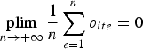 $$\mathop {{\rm plim}}\limits_{n \to + \infty} \displaystyle{1 \over n}\mathop \sum \limits_{e = 1}^n {o_{ite}} = 0$$
In this design, the average score among the nine experts for each wine is thus a consistent estimator of the objective score. We estimate the following price model:
 $$\ln ({\,p_{it}}) = \gamma {\overline {score} _{it}} + \delta t + {\mu _i}$$
where p it is the price of the wine of age t of producer i,  ${\overline {score} _{it}}$ is its average score among the nine experts, and μ i is the fixed effect of producer i.Footnote 3 These fixed effects aim to capture the effect of reputation on prices given the score and the age. The coefficient δ measures the storage cost, the quality improvements due to the keeping, and the scarcity value all at once. Remember that the data are a cross section, which means that the vintage, t of wine i, determines solely the age.
We estimate equation (2) with the generalized least squares (GLS). We use the Newey-West variance estimator, since the residuals faced both heteroscedasticity (the variance of the errors differs among producers) and autocorrelation (there is some inertia across vintages). The  ${\hat \gamma} $ obtained with the average score is compared to those obtained when we replace the average score with the score of a few major experts. We then use a subsample of wines that have been graded by at least the four main experts. One of these experts is Robert Parker (The Wine Advocate, WA), who enjoys a reputation as a wine guru with great influence on prices (Ali et al., Reference Ali, Lecocq and Visser2008; Jones and Storchmann, Reference Jones and Storchmann2001). Others include the Wine Spectator (WS), Jancis Robinson (JR), and Stephen Tanzer (International Wine Cellar, IWC). This cut leaves us with 737 prices of wines from 137 châteaux of Bordeaux, with vintages from 2000 to 2010. The use of this subsample allows us to conduct a multi-expert regression that controls for the correlations between the experts' grades. In the expert-specific regressions, the impacts of the different experts are not taken into account simultaneously, although the real impacts are indeed linked to one another. We therefore obtain more accurate estimates of experts' respective influences. This also provides an idea of the error made when only one expert is considered.
B. The Two-Stage Model
This naive model has some major limitations. The first one is the application of the LLG with at most nine experts for each wine. As Lecocq and Visser (Reference Lecocq and Visser2006) pointed out, it seems hardly acceptable that the opinions of the nine experts correct each other perfectly. Worse, the opinions o ite must be i.i.d. in order to validate the LLG. That is problematic since the grading behavior of experts depends on both their taste and their grading scale. As we shall see, some experts grade systematically using the average score and others grade systematically above the average. Given that information, this first model should be abandoned.
Another key limit of the naive model is that it assumes that the opinions have no influence on price. The underlying hypothesis is that the price is determined solely by the objective component of the scores, while the subjective component is irrelevant to the price equation. This point is mostly unacceptable, since the only observable score comprises both the objective and the subjective components. Moreover, some consumers might be interested in the differentiated opinions of the experts, acknowledging that each expert has his own tastes. This point has been highlighted by Lecoq and Visser (Reference Lecocq and Visser2006). When a consumer feels well represented by one expert, he is likely to be deeply influenced by the subjective opinion of this expert and might not look at the comments of the others.
We have shown the necessity of integrating the objective and subjective components in the price equation. Of course, this is achieved by using the raw scores, but this specification implies that the two components have the same coefficient. Testing this hypothesis is another goal of the present article. Hence, we need to disentangle q it from o ite in equation (1). To this end, we use the weather data as determinants of quality and identifying variables.
It seems reasonable to assume that quality is determined solely by the soil quality, the skills of the producer (including the viticulture ability, the reaper's precision during harvest, the maturation process, and the varietal blend), and the weather conditions during growth. Making the assumption that the two first factors can be captured by producer-specific fixed effects and a trend, we design the following model of objective quality:
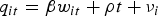 $${q_{it}} = \beta {w_{it}} + \rho t + {\nu _i}$$
where w it is the vector of the weather variables, and ν i is the fixed effect of the producer i on quality. In this design, the fixed effects are indicators of soil quality and producer skills. The trend aims to take into account the global improvements in technology. In order to limit the number of coefficients, we assume that the impact of the weather variables on the objective scores is the same for all producers.
We obtain the reduced form of scores by combining equations (1) and (3):
 $$scor{e_{ite}} = \beta {w_{it}} + \rho t + {\mu _i} + {o_{ite}}$$
which can be estimated using the GLS, thereby minimizing variation among the opinions. Again, we use the Newey-West variance estimator, as the opinions o ite showed heteroscedasticity and autocorrelation.
This first-stage regression gives us an estimate  ${\hat {\!o}_{ite}}$ of the opinions of the experts. Let
  ${\hat {\!o}_{it}}$ be the vector that includes the
  ${\hat {\!o}_{ite}}$. Adding this variable to the model (2) and replacing the average score with any expert score allows us to estimate the differentiated impacts of quality and experts' opinions on prices. This is stated formally as follows:
 $$\ln ({\,p_{it}}) = \gamma scor{e_{it{e_1}}} + \theta \,{\hat {\!o}_{it}} + \lambda t + {\rm \mu _i}$$
where e 1 is the chosen reference expert, and μi still aims to estimate the influence of reputation of producer i on price given the scores. Splitting the variable  $scor{e_{it{e_1}}}$ into its objective component
  ${\hat {\!q}_{it}}$ and its subjective component
  ${\hat {\!o}_{it{e_1}}}$, we get the detailed effects of scores on prices:
 $$\ln ({\,p_{it}}) = \gamma \,{\hat {\!q}_{it}} + (\gamma + {\theta _1})\,{\hat {\!o}_{it{e_1}}} + {\theta _2}\,{\hat {\!o}_{it{e_2}}} + \;. \;. \;. \; + {\theta _n}\,{\hat {\!o}_{it{e_n}}} + \lambda t + {\rm \mu _i}$$
where n is the number of experts. That is why the choice of expert does not matter. The coefficients are estimated using the bootstrap method to correct the sampling error in the ordinary least squares (OLS) variance estimates in the second stage (due to the replacement of (q, o) by $\left( {\hat {\!q},\hat {\!o}} \right)$). That is, we randomly draw with replacement a same-size subsample from the initial one, we conduct the two-stage estimation with this subsample, and we obtain the second-stage estimates that are calculated using OLS. We do this procedure 1,000 times and find that the convergent bootstrap estimate is the mean value of each coefficient. The variances in the bootstrap estimates are calculated nonparametrically using the empirical variance of the 1,000 estimates for each coefficient.
At this point, we should draw the link between our approach and instrumental variable techniques. Here, we use the weather data, the age of the wine, and producers' dummy variables as instruments for the raw scores. This IV procedure was used and discussed in Haeger and Storchmann (Reference Haeger and Storchmann2006). Our method is slightly different, however, since we use the residuals of this first-stage equation as a control variable for the second stage. Some tests are required to check our model:
- an endogeneity test, which is easily achieved by performing a t-test on the coefficient θe,
- an overidentification test, which is achieved by performing a Sargan test.
We provide these tests by bootstrapping the test statistics.
This procedure was first conducted on the entire sample by using only the mean score for each wine: this includes all wines graded by at least by one expert. Then we conduct the same analysis separately for each expert. As we did for the naive model, at the end we use the subsample of the 737 wines for further inter-expert analysis and as a robustness check. We compare these results to the naive model estimates.
C. Consumer Defiance Versus Marketing Effect
Our design allows us to provide precise estimates of the individual impacts of each expert, apart from the impact of the objective component of the scores. Yet it misses one indirect effect of the scores on price. As is often argued in the literature on marketing and consumer behavior (see, e.g., Martin-Consuegra et al., 2007), the standard deviation of grades is likely to negatively affect the buyer's trust in the scores. Assuming the consumer's risk aversion, a high dispersion of the scores decreases the equilibrium price because it lowers demand.
However, another indirect effect of the standard deviation on prices might occur. As shown by Hilger et al. (Reference Hilger, Rafert and Villas-Boas2011), when a retailer displays a score for a wine, its sales (or price) increase: the higher the exhibited score, the higher the increase in sales. A high standard deviation in scores for a wine implies that at least one expert liked the wine more than the others and gave it an above-average mark. Retailers know all the scores and can choose to talk about only the best. We call this positive correlation between the standard deviation of the scores and wine prices the “marketing effect.” The higher the standard deviation, the greater the likelihood that the retailer will display a good score (compared to the average) and the higher the price. Unexpectedly, the lack of consensus among experts allows retailers to improve their marketing and to increase their prices.
Our model allows us to test this hypothesis. Because the standard deviation of the scores is the standard deviation of the opinions, we add the latter to the regressors in the second stage of the multi-expert regression. To this end, we use the empirical standard deviations of estimated opinions for each wine as an estimate of the real deviation of the scores. The estimate of the coefficient and its related significance are obtained by bootstrap. We conduct this analysis on the subsample of 737 wines graded by all the experts, in order to maintain a constant number of grades per observation.
III. Data
Annual data were obtained for 203 wine producers, located mainly in the Bordeaux area (187 producers from 12 Appellation d'Origine Contrôlée (AOC) areas, with nine producers from Napa Valley, California, and seven from Spain) covering the period from 2000 to 2010. The prices were obtained from the website winedecider.com. This website offers prices on a wide range of wines from several countries and AOCs and is representative of the main wine sellers on the Internet, including Millesima. Here the listed price is the average retail price of a bottle packaged in a case of six or 12 bottles in 2011 prices before value-added tax (VAT) and transportation costs. Using the retail price means we can assume that these wines are priced after the experts have published their scores. This point is crucial to the relationship between wine prices and expert opinion. A retailer's pricing behavior will vary depending on whether he is aware of the expert ratings.
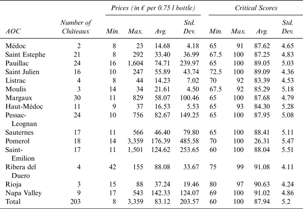
Table 1 provides descriptive statistics about the prices and the scores among the different appellations.
Table 1 2011 Prices and Scores Across Appellations

Source: Winedecider.com (as of the last week of May 2011).
Note: Scores are based on the average note given by the website for each château-vintage combination. For instance, the first line (Medoc) contains two wines, thus the statistics are given for 2 wines and 11 vintages (2000 to 2010), i.e., 22 observations. The prices correspond to the price of each château-vintage combination.
As in the hedonic approach, we include:
- Objective characteristics: name of the producer and vintage;
- Taste rating or subjective quality: scores from nine experts (each wine is graded by 4.5 experts on average);
- Weather as a determinant of objective quality: temperature and rainfall data from several meteorological stations in the heart of the AOC, due to the great heterogeneity of local weather conditions across the vast wine-producing area of Bordeaux (discussed below)
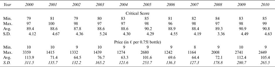
Table 2 examines the evolutions of the descriptive statistics in Table 1 on the entire sample of wines, across the several different vintages.
Table 2 Prices and Scores Across Vintages
Source: Winedecider.com.
Note: Min and max are calculated on the average score given by the winedecider.com website for each château-vintage combination, rounded to the nearest integer. S.D. = standard deviation.
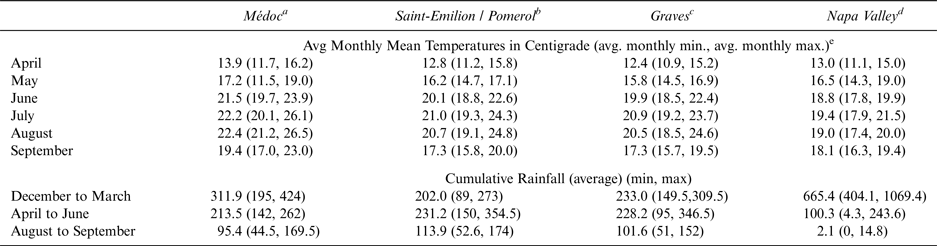
As for weather data, we obtain details of daily weather conditions for the three main areas of the Bordeaux region and for the Napa Valley. We define the three main climate areas of the Bordeaux appellations: Médoc, Saint-Emilion/Pomerol, and Graves. Meteorological studies related to wine reveal significant weather variability within the Bordeaux appellation (Bois, Reference Bois2007; Bois and Van Leeuwen, Reference Bois and Van Leeuwen2008). Table 3 shows the average temperatures and rainfalls across the four available stations in the areas.
Table 3 Descriptive Statistics of Weather Variables (2000–2010)
Sources: a weather station of Château Latour; b weather station of Château Grand Barrail; c weather stations of Château Haut-Bergey; d Monthly Report of California Irrigation Management Information System, Oakville weather station (CIMIS #77, Oakville), wwwcimis.water.ca.gov. e) averages of monthly means over 11 years.
Consistent with Bois and Van Leeuwen's (Reference Bois and Van Leeuwen2008) climate observations, this information is crucial to our study. It is essential to correlate not only data from the main meteorological station based in Mérignac but also the meteorological data from each of these three areas in the Bordeaux region. Although Lecocq and Visser (Reference Lecocq and Visser2006) show that the Mérignac station provided a reasonably acceptable proxy of the weather for the Bordeaux appellation as a whole between 1993 and 2002, they note the appearance of some differences: “The climate conditions prevailing in the main weather station [Mérignac] are thus clearly not representative of the Bordeaux wine region as a whole” (Lecocq and Visser, Reference Lecocq and Visser2006, p. 6). Our model aims to use meteorological data as an instrument for the scores. Consequently, if we want to maintain some heterogeneity in our fitted scores, we cannot use only one station.
We have gathered the monthly temperatures and levels of rainfall from three stations representative of the three main wine regions of Bordeaux. For the Médoc region, we use weather data from Château Latour (which is very close to Pauillac). In the Graves region, we use weather data from Château Haut-Bergey (in Léognan). For Saint-Emilion/Pomerol, we use data from Château Grand Barrail. All these weather stations are located directly in the vineyards. Our data for the Napa Valley refer to the Oakville meteorological station, which is located only in close proximity to vineyards. The exact location within certain meso-climates may explain the surprising fact that our Napa temperatures are below those in Bordeaux. We do not have weather conditions for the two Spanish appellations.
IV. Empirical Results
A. Results from the Naive Model
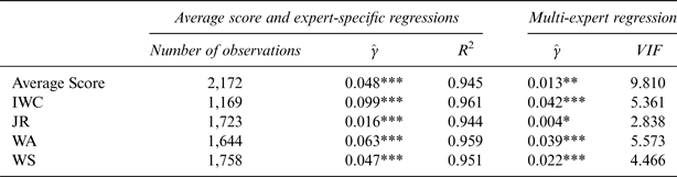
Table 4 gathers the γ estimates for the naive model.Footnote 4 We have estimated equation (2) first using the average of all available scores and then using scores from each of these experts. For these expert-specific regressions, we provide the number of observations and the coefficient of determination (R 2). Table 4 also lists the estimates of the multi-expert regression, including the average score. The last column shows the Variance Inflation Factors (VIFs), indicating potentially weak multicollinearity issues for the average score coefficient.
Table 4 Naive Model γ Estimates of Equation (2)
Note: The columns  $\hat \gamma $ contain the estimated influence of the average score and the experts on price for the two different specifications. Significance levels: ***1%, **5%, *10%.
The main observation is that the estimate of γ is significantly dependent on the specification of scores. The results displayed in column 3 underline the importance of using several experts in order to model wine prices, since they all have differentiated impacts.Footnote 5 According to the naive model, a one-point-increase in the objective score leads to a 4.8% increase in prices. Note that the coefficient of determination is not the highest for the average score model though it should be the best model. This suggests that the subjective opinions of the experts contribute to determining wine prices, which would invalidate the naive model.
The hierarchy of experts' influence is remarkably the same in the two models. In particular, Robert Parker (WA) is not the most influential expert: he is second to Stephen Tanzer (IWC). Both models conclude that Jancis Robinson (JR) has minimal influence and Wine Spectator (WS) has average impact . This is consistent with the results of Ashton (Reference Ashton2013) regarding correlations between experts: he found that JR was the most “out of line” expert and that her taste differed the most from that of WA.
B. The Two-Stage Model Results
(1) First Stage
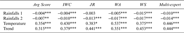
Table 5 shows the first-stage estimates related to equation (4), for each single-expert regression, for the average score regression, and for the multi-expert regression. We have tried numerous aggregated specifications of the weather data, since the estimates of the raw monthly temperatures and rainfalls coefficients were found to be rather inconsistent. We display the results using the following aggregates, which give the most robust and significant results:Footnote 6
- The total rainfall during the first part of the growing season: April to July (referred to as Rainfall 1),
- the total rainfall during the last part of the growing season: August and September (referred to as Rainfall 2),
- the average of the monthly average temperatures during the growing season (from April to September, referred to as Temperature).
Table 5 First-Stage Estimates of Equation (4)
Note: Five separate regressions explaining each expert score and the average score by referring to weather and a trend variable; multi-expert regression explaining the expert scores altogether with the same explanatory variables. Significance levels: ***1%, **5%, *10%.
We divided the growing season into two parts for the rainfall, because of the major expected impact of rainfall in the final months of the growth. At this point of growth, intense rainfall causes the grapes to rot, which jeopardizes the quality of the crop. To a lesser extent, rainfall still negatively affects the quality of the vintage during the rest of the growth season. The temperature showed important multicollinearity issues, which is why we focused on the average temperature during the growth season. We also show the estimated coefficients related to the trend, which is seen as the impact of overall progress in technology.
The signs of the coefficients are consistent with the literature in phenology: a good vintage is caused by a dry summer, with a high temperature. As expected, rainfall during August and September have a greater negative impact than rainfalls at the beginning of the growing season. This trend is also very significant, indicating great progress in technology through the trend in the scores.
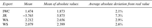
As a clue to the accuracy of the first-stage fitted values, in Table 6 we provide some descriptive statistics of the residuals of the multi-expert regression. Column 2 displays the mean opinion for each expert, column 3 displays the mean of the absolute values, and column 4 gives the average deviation from the real value in percentage.
a see also last column of Table 5.
Column 1 shows that JR is, on average, far below the mean score. This is due to the fact that she originally grades on a scale of 20 and that we remapped these grades onto a 100-point scale in order to create homogeneity among the results. At the opposite end of the spectrum, WA, WS, and IWC are generally above the mean score. This regression is fairly accurate, since scores are estimated with an average error ranging from 2.1% for IWC to 7.3% for JR. Recall that our goal here is not the precise estimation of the scores but, rather, estimation of the residuals. The accuracy of the first-stage regression is not the issue, since we actually expect some heterogeneity in the residuals.
(2) Second Stage
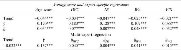
We now comment on the estimates of equation (5). Table 7 displays the bootstrap estimates for each expert-specific regression, for the average score regression, and for the multi-expert regression. None of the non-reported Sargan tests for overidentification allow rejection of the exogeneity of the instruments at the of 5% level. Hence, the exclusion condition for the validity of our instruments cannot be rejected.
Table 7 Second-Stage Estimates of Equation (5)
Note: Five separate augmented regressions explaining the prices by referring to fitted scores and first-stage residuals for each expert and the average score; multi-expert augmented regression explaining prices by referring to fitted score and all residuals for each expert from multi-expert first-stage. In the upper part,  $\hat \gamma $ contains the estimated influence of the objective score using either only the average score or only a specific expert, leading to six different estimates of the same value.
  $\hat {\!\theta} $ contains the estimated influence of the subjective scores for each regression. In the lower part, we show the same estimates obtained with the multi-expert regression, leading to only one estimate for the influence of the objective score (
 $\hat \gamma $). Significance levels: ***1%, **5%, *10%.
The results definitely reject the naive model as suitable for assessing the impact of the objective component of scores. Indeed, each of the subjective components included in any of the specifications has a significant impact on wine pricing. The naive model aims to dispose of the opinions in order to focus on the objective scores, but these opinions have a significant impact on prices. The naive model is thus flawed: the  ${\hat \gamma} $ displayed in Table 4 are all negatively biased. Two sources of bias are observed: the LLG is not valid because the opinions are not i.i.d., and the subjective components have a significant impact on prices. In addition, the systematic significance of the opinions also confirms the endogeneity of the raw scores and supports our two-stage model.
Furthermore, the opinions have different impacts. This means that one should use different experts in order to properly estimate the impact of the objective component, because they all influence wine prices in their own way. This is illustrated by the dispersion among the  $\hat {\!\gamma }$ obtained in the average score and expert-specific regressions (upper part of Table 7). Note that the hierarchy of the experts is still robust: IWC and WA are the most influential experts, and JR is the least.
All the  $\hat {\!\gamma }$ obtained with the two-stage procedure are much greater than those obtained with the naive model. This can be explained both by the downward measurement error bias (see Chesher, Reference Chesher1991; Lecocq and Visser, Reference Lecocq and Visser2006) and by the omitted variable bias, as the opinions are positively correlated with wine prices and mainly negatively correlated with the objective scores. It supports the use of our model to avoid those two biases. Note that the
  $\hat {\!\gamma }$ coefficients are also greater than their related
  ${\hat {\!\theta}} $ coefficients. This indicates that the objective component of the scores is more influential than the subjective one. In other words, our conclusions show that prices are determined more precisely by the fundamentals than by the subjective opinions of experts.
Another feature of these estimates is that the expert's respective influences are slightly lower in the multi-expert regression than in the naive model. This is consistent with Dubois and Nauges (Reference Dubois and Nauges2010), who also found an upward bias of the estimated influences when the unobserved quality, or the objective score as we call it here, are not controlled for. In our model, a one-point increase in the objective score is estimated to have a 13.7% impact on the price, whereas a one-point increase in the experts' opinion has a maximum impact of 4.5% on the price for IWC, 4.1% for WA, and 0.4% for JR. Indeed, these are purely visions, as we cannot observe the two components of the scores.
Finally, the trend is also very significant: in the multi-expert regression, we estimate that a wine becomes 2.2% more expensive each year due to storage costs, maturation, and scarcity value.
C. Marketing Effect
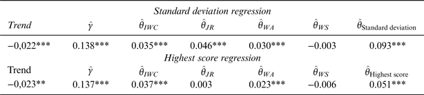
As an application of our model, we test the impact of the deviation among the scores on prices. Digressing slightly from our structural model, we add the empirical standard deviation of the opinions to equation (5) to assess the significance of its coefficient and the sign of the latter. The upper part of Table 8 shows the results of this estimation.
Table 8 Second-Stage Estimates of the Multi-Expert Design
Note: The interpretation of the estimates is the same as for the lower part of Table 7 except for the last column.  ${\hat {\!\theta} _{{\rm Standard\; deviation}}}$ and
  ${\hat {\!\theta} _{{\rm Highest\; score}}}$ refer to the respective influence of the empirical standard deviation of the opinions and of the highest score.
Significance levels: ***1%, **5%, *10%.
The model indicates a strong positive impact of the standard deviation of experts' opinions on the prices of wines. That correlation might result from what we introduced as the “marketing effect” in section II.C. In that case, we should find that the highest score has a major impact and is supposed to be the most publicized, hence the most important in the price equation.
We test this hypothesis by comparing the highest score to all the individual opinions in the two-stage model. The results of this estimation are displayed in the lower part of Table 8. The coefficient of the highest score is estimated to be the most important one. This is an argument in favor of the “marketing effect” interpretation. The highest score is the score most often exhibited , so it is the only hint of quality for consumers who have not searched for the other experts' grades (Hilger et al., Reference Hilger, Rafert and Villas-Boas2011). Therefore, the highest score has the greatest influence on the price.Footnote 7
The revealed impact of the highest score sheds new light on the respective influence of the experts. The idea of a marketing effect with regard to the diffusion of scores might explain why JR is deemed to have so little influence on prices. Because she often grades below the average, many sellers might not be eager to exhibit her scores. At the same time, the fact that WA and WS are usually above the mean score might play a role in their larger influence. This interpretation is consistent with the results of Table 8: the introduction of the highest score in the regression has lowered the coefficients of the above-the-mean-score experts.
V. Conclusion
This research aims to assess the role of expert opinion on Bordeaux wine prices using a methodology that, by including detailed meteorological data, fixed-effects models, and the systematic use of numerous expert scores, avoids endogeneity and bias rooted in errors of judgment. Like Dubois and Nauges (Reference Dubois and Nauges2010), Lecocq and Visser (Reference Lecocq and Visser2006), and Oczkowski (Reference Oczkowoski2001), we assume that the observed scores result from an error measurement model: they can be split into an objective component shared by all experts and a subjective component specific for each expert and each wine. The latter is often seen as something that should be corrected because it obscures the signs of quality indicated by the objective component. We provide evidence, however, that in a price equation one should not try to get rid of subjective components because they significantly affect wine prices. Worse, if not handled specifically, the correction of these components leads to downward-biased estimates of the impact of the scores as a quality indicator for wine prices. This result is consistent with Lecocq and Visser (Reference Lecocq and Visser2006).
The most important result of our findings is the light shed on the role of the standard deviation in the price equation. We find a strong positive correlation between wine pricing and the standard deviation of the scores. Our interpretation is based on the fact that a higher standard deviation indicates that at least one score is above the others. In line with the marketing literature, this highest score might be used in an advertisement by the sellers. Hence, this particular score is likely to be the most publicized. As a result, this is certainly the only score that the average consumers have heard of. This is what we call the “marketing effect”: the highest score is the most influential because it is the best known among consumers. Our interpretation is supported by the empirical analysis, since the highest score has the greatest impact on prices.
Nonetheless, we have to be cautious about this interpretation. There is another interpretation of our results: the consumers might be risk-takers. In this case, the standard deviation of the scores should also have a positive influence on demand and thus on prices. Economists generally agree that the ordinary consumer is rather risk averse, but the market we discuss here is very specific. The prices in our data range from $8 to $3,000, and the average price is $83. This is no market for the uninitiated. The consumers involved in this market are connoisseurs, professionals, or investors, and at least the last of these are likely to be risk-takers. However, we maintain our interpretation, assuming that market prices are more likely to be influenced by the marketing effect than by risk-taking behavior.
Appendix
Appendix Table 1 Experts' Scores