


1 Introduction
A real rough fracture is usually characterized by a heterogeneous structure composed of aperture zones and localized contact spots. Modelling of the fluid transport properties of channels having such complex topographies can be a challenging problem due to their multiscale nature. Indeed, the domain under study can have a length scale of the order of a few millimetres or more, while containing influential details down to the micrometre or less (Lorenz & Persson Reference Lorenz and Persson2009; Dapp & Müser Reference Dapp and Müser2016). Yet, the transport properties of such fractures represent a critical issue in many industrial applications as they can determine their success or failure. For example, one can cite the flow study through fractured rocks (Mourzenko, Thovert & Adler Reference Mourzenko, Thovert and Adler1995; Berkowitz Reference Berkowitz2002) for fluid recovery and for integrity of caprocks or for the leak rate determination of metal-to-metal mechanical seals (Marie et al. Reference Marie, Lasseux, Zahouani and Sainsot2003; Marie & Lasseux Reference Marie and Lasseux2007; Vallet et al. Reference Vallet, Lasseux, Sainsot and Zahouani2009; Ledoux et al. Reference Ledoux, Lasseux, Favreliere, Samper and Grandjean2011; Pérez-Ràfols, Larsson & Almqvist Reference Pérez-Ràfols, Larsson and Almqvist2016) intervening in the design of nuclear power plants or in ultrahigh vacuum applications among many others (Lefrançois Reference Lefrançois2004).
Noticing that, in general, the typical length scale of the roughness pattern is much smaller than the macroscopic size of the domain, many authors have thus been interested in a scale separation approach to describe an average flow model rather than a deterministic solution at the roughness scale. This was first addressed in the context of surface lubrication by splitting the problem into two scales, that is, a global scale and a smaller one taking into consideration the details at the roughness level. Moreover, when it is assumed that the local slopes of the roughness are small, the lubrication assumption holds and the flow is described by the Reynolds equation at the microscopic scale. Interested in the effect of a one-dimensional longitudinal or transverse roughness pattern on the flow, Christensen (Reference Christensen1970) developed a model based on statistical averaging of the Reynolds equation. Later, Patir & Cheng (Reference Patir and Cheng1978) published a study for a more general roughness structure while taking into account the possible contact between the surfaces. This analysis resulted in the inclusion of scalar ‘flow factors’ in the macroscale Reynolds equation to model the effect of roughness on the flow, thus making a link between the two scales of the problem. This concept has been extended by Tripp (Reference Tripp1983), who used a stochastic approach, while Prat, Plouraboué & Letalleur (Reference Prat, Plouraboué and Letalleur2002) made use of the method of volume averaging to obtain an averaged Reynolds equation involving a tensorial transmissivity. Such a formulation allows the description of the average flow for anisotropic roughness and basically reduces to Patir and Cheng’s model when the off-diagonal terms of the transmissivity tensor vanish, i.e. when expressed in the principal axes of the fracture. Fractures in geological formations can exhibit more complex structures for which the scale separation, from the scale of asperities to that of the fracture itself, is not always fulfilled. Moreover, fractures in this kind of material are often organized in complex networks (see Tsang & Tsang (Reference Tsang and Tsang1987), Lee, Lough & Jensen (Reference Lee, Lough and Jensen2001) and references therein), requiring careful attention for a proper description at the scale of an entire fracture or fracture network. Nevertheless, our approach developed below is restricted to the first upscaling, from the scale of asperities to that of a local element characterized by a local transmissivity, for which scale separation does not usually represent a critical constraint. In many other configurations, this constraint is even easily satisfied, such as, for instance, in assemblies of machined surfaces. Machining operates an upper cutoff on the characteristic size of asperities so that their scale is distinctly separated from that of waviness (Stout, Davis & Sullivan Reference Stout, Davis and Sullivan1990; Stout et al. Reference Stout, Blunt, Dong, Mainsah, Luo, Mathia, Sullivan and Zahouani2000; Stout & Blunt Reference Stout and Blunt2013), a sufficient requirement for this first upscaling to be applied. Further upscaling procedures, similar to the one developed here, can be envisaged to account for defaults at larger scale if appropriate.
Most of the work reported so far has concentrated on the flow of an incompressible liquid. In this work, interest is focused on the single-phase pressure-driven flow of a slightly compressible fluid between confined rough walls. When the aperture of the fracture is comparable to the mean free path of the fluid, a rarefaction effect (or Knudsen effect) may appear, which can significantly impact the mass, momentum and heat transfer through the aperture field. The existence of this flow regime can be characterized by the value of the Knudsen number,
 $Kn$
, defined as the ratio of the mean free path of the gas molecules at the pressure and temperature under consideration to a characteristic constriction length. According to Karniadakis, Beskok & Aluru (Reference Karniadakis, Beskok and Aluru2005), when
$Kn$
, defined as the ratio of the mean free path of the gas molecules at the pressure and temperature under consideration to a characteristic constriction length. According to Karniadakis, Beskok & Aluru (Reference Karniadakis, Beskok and Aluru2005), when
 $10^{-2}\lesssim Kn\lesssim 10^{-1}$
, the so-called slip flow regime is reached and the Navier–Stokes equations together with the classical no-slip boundary condition fail to model the rarefied flow properly. This is circumvented by introducing a finite slip velocity at the walls while the classical mass and momentum conservation equations remain the same as in the continuum regime (i.e. when
$10^{-2}\lesssim Kn\lesssim 10^{-1}$
, the so-called slip flow regime is reached and the Navier–Stokes equations together with the classical no-slip boundary condition fail to model the rarefied flow properly. This is circumvented by introducing a finite slip velocity at the walls while the classical mass and momentum conservation equations remain the same as in the continuum regime (i.e. when
 $Kn\lesssim 10^{-2}$
). Such a situation has been particularly studied in micro- and nanofluidic devices (Porodnov et al.
Reference Porodnov, Suetin, Borisov and Akinshin1974; Arkilic, Schmidt & Breuer Reference Arkilic, Schmidt and Breuer1997; Beskok & Karniadakis Reference Beskok and Karniadakis1999; Cai, Sun & Boyd Reference Cai, Sun and Boyd2007; Dongari, Agrawal & Agrawal Reference Dongari, Agrawal and Agrawal2007) or for gas flow in porous media for instance (Klinkenberg Reference Klinkenberg1941; Skjetne & Auriault Reference Skjetne and Auriault1999; Lasseux et al.
Reference Lasseux, Valdes Parada, Ochoa Tapia and Goyeau2014; Lasseux, Valdés Parada & Porter Reference Lasseux, Valdés Parada and Porter2016). The concept of a linear or first-order slip velocity boundary condition was initially introduced by Navier and later improved by Maxwell (Reference Maxwell1879). It is such that the slip velocity is tangential to the wall and proportional to the local shear rate. So as to increase the Knudsen number range of applicability of the slip regime, second-order and more general slip boundary conditions have been introduced (Karniadakis et al.
Reference Karniadakis, Beskok and Aluru2005), but may result in an erroneous velocity distribution along with numerical implementation difficulties (McNenly, Gallis & Boyd Reference McNenly, Gallis and Boyd2005). Hence, our objective in this article is to carefully derive a macroscopic model operating at the scale of a representative elementary portion of the fracture for slightly compressible slip flow (i.e. for sufficiently small values of the Knudsen number). To this end, the flow will be described by the classical continuum-based mass conservation and Navier–Stokes equations along with a Maxwell-type first-order slip boundary condition at the walls.
$Kn\lesssim 10^{-2}$
). Such a situation has been particularly studied in micro- and nanofluidic devices (Porodnov et al.
Reference Porodnov, Suetin, Borisov and Akinshin1974; Arkilic, Schmidt & Breuer Reference Arkilic, Schmidt and Breuer1997; Beskok & Karniadakis Reference Beskok and Karniadakis1999; Cai, Sun & Boyd Reference Cai, Sun and Boyd2007; Dongari, Agrawal & Agrawal Reference Dongari, Agrawal and Agrawal2007) or for gas flow in porous media for instance (Klinkenberg Reference Klinkenberg1941; Skjetne & Auriault Reference Skjetne and Auriault1999; Lasseux et al.
Reference Lasseux, Valdes Parada, Ochoa Tapia and Goyeau2014; Lasseux, Valdés Parada & Porter Reference Lasseux, Valdés Parada and Porter2016). The concept of a linear or first-order slip velocity boundary condition was initially introduced by Navier and later improved by Maxwell (Reference Maxwell1879). It is such that the slip velocity is tangential to the wall and proportional to the local shear rate. So as to increase the Knudsen number range of applicability of the slip regime, second-order and more general slip boundary conditions have been introduced (Karniadakis et al.
Reference Karniadakis, Beskok and Aluru2005), but may result in an erroneous velocity distribution along with numerical implementation difficulties (McNenly, Gallis & Boyd Reference McNenly, Gallis and Boyd2005). Hence, our objective in this article is to carefully derive a macroscopic model operating at the scale of a representative elementary portion of the fracture for slightly compressible slip flow (i.e. for sufficiently small values of the Knudsen number). To this end, the flow will be described by the classical continuum-based mass conservation and Navier–Stokes equations along with a Maxwell-type first-order slip boundary condition at the walls.
This paper is organized as follows. Assuming that the local slope of the fracture walls is everywhere small compared with unity, the first-order slip-corrected Reynolds equation is derived in § 2, starting from the microscale Stokes and continuity equations along with a first-order slip boundary condition at the walls. Then, the upscaling process is applied to the Reynolds equation in § 3, making use of the method of volume averaging and leading to the macroscopic flow model and to a closure problem that is to be solved to obtain the effective transmissivity tensor. An expansion of the closure problem at the first order in the Knudsen number is then performed to identify purely viscous and slip-correction effects separately. In § 4, numerical solutions to the closure problem, along with a comparison between the macroscopic model and its first-order approximation on a randomly rough fracture, are presented. The dependence of the macroscopic transmissivity tensor on the Knudsen number that appears in the average flow model is portrayed. Finally, conclusions of this study are proposed in § 5.
2 Microscale physical model
2.1 Scale analysis and simplified governing equations
The situation under consideration in this work is that of a stationary isothermal slightly compressible one-phase flow of a barotropic gas in a fracture made up of two rough surfaces. Moreover, the viscous flow is assumed to occur at small Reynolds number (creeping flow) so that it can be described by the Stokes equation at the roughness level. This can be shown starting from the compressible Navier–Stokes equations and performing an order of magnitude analysis on the different terms using length-scale constraints (see Quintard & Whitaker (Reference Quintard and Whitaker1996) and Lasseux et al. (Reference Lasseux, Valdes Parada, Ochoa Tapia and Goyeau2014) for the details). A first-order slip boundary condition is assumed at the solid–fluid interface, making the fluid velocity locally tangential to the wall. Such a condition takes the form of (2.1d ) as proposed in Lauga, Brenner & Stone (Reference Lauga, Brenner and Stone2007). Under these circumstances, while neglecting the effect of body forces, the flow can be described by the following set of equations:
 $$\begin{eqnarray}\displaystyle & \displaystyle \unicode[STIX]{x1D735}\boldsymbol{\cdot }(\unicode[STIX]{x1D70C}\boldsymbol{v})=0\quad \text{in }\unicode[STIX]{x1D6FA}_{\unicode[STIX]{x1D6FD}}, & \displaystyle\end{eqnarray}$$
 $$\begin{eqnarray}\displaystyle & \displaystyle -\unicode[STIX]{x1D735}p+\unicode[STIX]{x1D707}\unicode[STIX]{x1D6FB}^{2}\boldsymbol{v}=0\quad \text{in }\unicode[STIX]{x1D6FA}_{\unicode[STIX]{x1D6FD}}, & \displaystyle\end{eqnarray}$$
 $$\begin{eqnarray}\displaystyle & \displaystyle \unicode[STIX]{x1D70C}=\unicode[STIX]{x1D711}(p)\quad \text{in }\unicode[STIX]{x1D6FA}_{\unicode[STIX]{x1D6FD}}, & \displaystyle\end{eqnarray}$$
 $$\begin{eqnarray}\displaystyle & \displaystyle \boldsymbol{v}=-\unicode[STIX]{x1D709}\unicode[STIX]{x1D706}\boldsymbol{n}\boldsymbol{\cdot }\left(\unicode[STIX]{x1D735}\boldsymbol{v}+\unicode[STIX]{x1D735}\boldsymbol{v}^{\text{T}}\right)\boldsymbol{\cdot }(\unicode[STIX]{x1D644}-\boldsymbol{n}\boldsymbol{n})\quad \text{at }{\mathcal{A}}_{\unicode[STIX]{x1D70E}\unicode[STIX]{x1D6FD}}. & \displaystyle\end{eqnarray}$$
In problem (2.1),
 $\unicode[STIX]{x1D6FA}_{\unicode[STIX]{x1D6FD}}$
designates the fluid phase domain,
$\unicode[STIX]{x1D6FA}_{\unicode[STIX]{x1D6FD}}$
designates the fluid phase domain,
 ${\mathcal{A}}_{\unicode[STIX]{x1D70E}\unicode[STIX]{x1D6FD}}$
is the solid–fluid interface,
${\mathcal{A}}_{\unicode[STIX]{x1D70E}\unicode[STIX]{x1D6FD}}$
is the solid–fluid interface,
 $\unicode[STIX]{x1D70C}$
and
$\unicode[STIX]{x1D70C}$
and
 $p$
are respectively the density and pressure,
$p$
are respectively the density and pressure,
 $\unicode[STIX]{x1D707}$
is the dynamic viscosity which will be considered constant throughout this work (i.e. the fluid is Newtonian) and
$\unicode[STIX]{x1D707}$
is the dynamic viscosity which will be considered constant throughout this work (i.e. the fluid is Newtonian) and
 $\boldsymbol{v}$
is the velocity, the components of which in the orthonormal basis
$\boldsymbol{v}$
is the velocity, the components of which in the orthonormal basis
 $(\boldsymbol{e}_{x},~\boldsymbol{e}_{y},~\boldsymbol{e}_{z})$
(see figure 1) are
$(\boldsymbol{e}_{x},~\boldsymbol{e}_{y},~\boldsymbol{e}_{z})$
(see figure 1) are
 $(u,~v,~w)$
. In (2.1d
),
$(u,~v,~w)$
. In (2.1d
),
 $\unicode[STIX]{x1D644}$
is the identity tensor,
$\unicode[STIX]{x1D644}$
is the identity tensor,
 $\boldsymbol{n}$
is the unit normal vector at
$\boldsymbol{n}$
is the unit normal vector at
 ${\mathcal{A}}_{\unicode[STIX]{x1D70E}\unicode[STIX]{x1D6FD}}$
pointing from the fluid phase
${\mathcal{A}}_{\unicode[STIX]{x1D70E}\unicode[STIX]{x1D6FD}}$
pointing from the fluid phase
 $\unicode[STIX]{x1D6FD}$
towards the solid phase
$\unicode[STIX]{x1D6FD}$
towards the solid phase
 $\unicode[STIX]{x1D70E}$
and the superscript
$\unicode[STIX]{x1D70E}$
and the superscript
 $\text{T}$
represents the transpose of a second-order tensor. Moreover,
$\text{T}$
represents the transpose of a second-order tensor. Moreover,
 $\unicode[STIX]{x1D706}$
denotes the mean free path of the gas molecules at the pressure and temperature under consideration and
$\unicode[STIX]{x1D706}$
denotes the mean free path of the gas molecules at the pressure and temperature under consideration and
 $\unicode[STIX]{x1D709}$
is a factor that depends on the tangential-momentum accommodation coefficient (TMAC),
$\unicode[STIX]{x1D709}$
is a factor that depends on the tangential-momentum accommodation coefficient (TMAC),
 $\unicode[STIX]{x1D70E}_{v}$
, as (Maxwell Reference Maxwell1879)
$\unicode[STIX]{x1D70E}_{v}$
, as (Maxwell Reference Maxwell1879)
 $$\begin{eqnarray}\unicode[STIX]{x1D709}={\displaystyle \frac{2-\unicode[STIX]{x1D70E}_{v}}{\unicode[STIX]{x1D70E}_{v}}}.\end{eqnarray}$$
The TMAC was introduced by Maxwell to account for the type of molecule-to-wall reflection and is related to the tangential component of the shear stress at the wall. A value of
 $\unicode[STIX]{x1D70E}_{v}=0$
is representative of a purely specular reflection, whereas
$\unicode[STIX]{x1D70E}_{v}=0$
is representative of a purely specular reflection, whereas
 $\unicode[STIX]{x1D70E}_{v}=1$
refers to a purely diffusive one. Experimentally,
$\unicode[STIX]{x1D70E}_{v}=1$
refers to a purely diffusive one. Experimentally,
 $\unicode[STIX]{x1D70E}_{v}$
ranges from
$\unicode[STIX]{x1D70E}_{v}$
ranges from
 $0.75$
to
$0.75$
to
 $0.85$
for various gases, yielding values for
$0.85$
for various gases, yielding values for
 $\unicode[STIX]{x1D709}$
between
$\unicode[STIX]{x1D709}$
between
 $1.3$
and
$1.3$
and
 $1.7$
(Arkilic, Breuer & Schmidt Reference Arkilic, Breuer and Schmidt2001; Karniadakis et al.
Reference Karniadakis, Beskok and Aluru2005; Ewart et al.
Reference Ewart, Perrier, Graur and Méolans2007), while the TMAC seems to increase with the molar mass of the gas (Graur et al.
Reference Graur, Perrier, Ghozlani and Molans2009). For the important application of CO
$1.7$
(Arkilic, Breuer & Schmidt Reference Arkilic, Breuer and Schmidt2001; Karniadakis et al.
Reference Karniadakis, Beskok and Aluru2005; Ewart et al.
Reference Ewart, Perrier, Graur and Méolans2007), while the TMAC seems to increase with the molar mass of the gas (Graur et al.
Reference Graur, Perrier, Ghozlani and Molans2009). For the important application of CO
 $_{2}$
sequestration, one finds values of
$_{2}$
sequestration, one finds values of
 $\unicode[STIX]{x1D70E}_{v}$
in the range mentioned above or even larger (Arkilic et al.
Reference Arkilic, Breuer and Schmidt2001; Agrawal & Prabhu Reference Agrawal and Prabhu2008). Obviously,
$\unicode[STIX]{x1D70E}_{v}$
in the range mentioned above or even larger (Arkilic et al.
Reference Arkilic, Breuer and Schmidt2001; Agrawal & Prabhu Reference Agrawal and Prabhu2008). Obviously,
 $\unicode[STIX]{x1D709}$
is a factor of the order of unity and, for practical purposes, it will be considered as a constant throughout this work.
$\unicode[STIX]{x1D709}$
is a factor of the order of unity and, for practical purposes, it will be considered as a constant throughout this work.
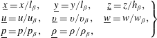
As sketched in figure 1, the fracture is composed of two rough surfaces which are both described by their heights
 $z=h_{i}(x,y)$
with respect to a reference set of coordinates; their normal unit vectors, which depend on the
$z=h_{i}(x,y)$
with respect to a reference set of coordinates; their normal unit vectors, which depend on the
 $(x,y)$
coordinates, are denoted by
$(x,y)$
coordinates, are denoted by
 $\boldsymbol{n}_{\boldsymbol{i}}(x,y)$
,
$\boldsymbol{n}_{\boldsymbol{i}}(x,y)$
,
 $i=1$
and
$i=1$
and
 $2$
for the bottom and top surfaces respectively. Furthermore, the local aperture field is denoted by
$2$
for the bottom and top surfaces respectively. Furthermore, the local aperture field is denoted by
 $h(x,y)=h_{2}(x,y)-h_{1}(x,y)$
, which can be positive or zero if contact occurs.
$h(x,y)=h_{2}(x,y)-h_{1}(x,y)$
, which can be positive or zero if contact occurs.
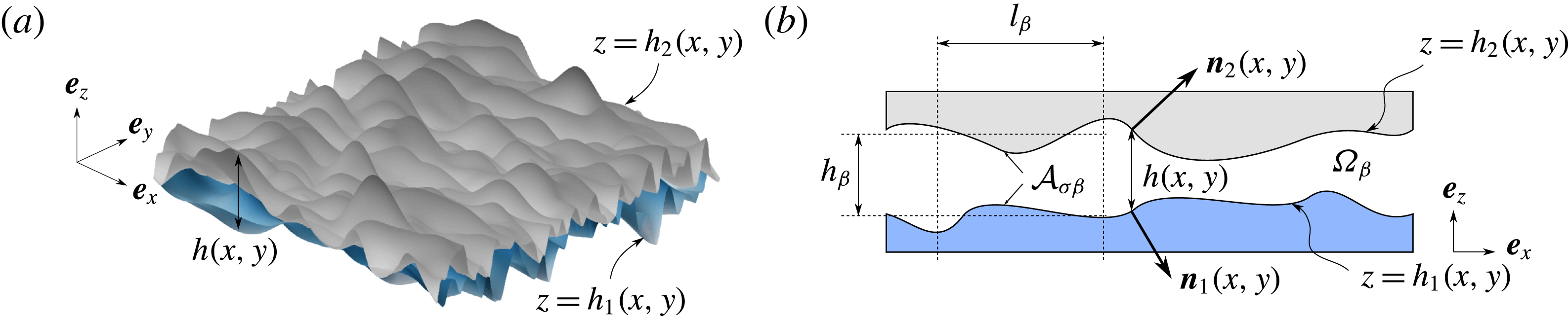
Figure 1. A fracture made of two rough surfaces and associated parameters.
If we assume that the aperture field is slowly varying with the in-plane coordinates
 $x$
and
$x$
and
 $y$
(i.e. that the slope of asperities is everywhere small compared with 1), it is of interest to derive the Reynolds equation from the problem (2.1). To this purpose, we introduce the following dimensionless quantities (denoted with an underline):
$y$
(i.e. that the slope of asperities is everywhere small compared with 1), it is of interest to derive the Reynolds equation from the problem (2.1). To this purpose, we introduce the following dimensionless quantities (denoted with an underline):
 $$\begin{eqnarray}\displaystyle \left.\begin{array}{@{}ccc@{}}\text{}\underline{x}=x/l_{\unicode[STIX]{x1D6FD}}, & \text{}\underline{y}=y/l_{\unicode[STIX]{x1D6FD}}, & \text{}\underline{z}=z/h_{\unicode[STIX]{x1D6FD}},\\[2.0pt] \text{}\underline{u}=u/u_{\unicode[STIX]{x1D6FD}}, & \text{}\underline{v}=v/v_{\unicode[STIX]{x1D6FD}}, & \text{}\underline{w}=w/w_{\unicode[STIX]{x1D6FD}},\\[2.0pt] \text{}\underline{p}=p/p_{\unicode[STIX]{x1D6FD}}, & \text{}\underline{\unicode[STIX]{x1D70C}}=\unicode[STIX]{x1D70C}/\unicode[STIX]{x1D70C}_{\unicode[STIX]{x1D6FD}},\end{array}\right\} & & \displaystyle\end{eqnarray}$$
where
 $l_{\unicode[STIX]{x1D6FD}}$
is the characteristic length scale over which the aperture field experiences significant variations in the
$l_{\unicode[STIX]{x1D6FD}}$
is the characteristic length scale over which the aperture field experiences significant variations in the
 $(x,y)$
directions while
$(x,y)$
directions while
 $h_{\unicode[STIX]{x1D6FD}}$
is the characteristic length scale of the aperture
$h_{\unicode[STIX]{x1D6FD}}$
is the characteristic length scale of the aperture
 $h$
. In addition,
$h$
. In addition,
 $u_{\unicode[STIX]{x1D6FD}}$
,
$u_{\unicode[STIX]{x1D6FD}}$
,
 $v_{\unicode[STIX]{x1D6FD}}$
and
$v_{\unicode[STIX]{x1D6FD}}$
and
 $w_{\unicode[STIX]{x1D6FD}}$
represent the characteristic velocity magnitudes in the
$w_{\unicode[STIX]{x1D6FD}}$
represent the characteristic velocity magnitudes in the
 $x$
,
$x$
,
 $y$
and
$y$
and
 $z$
directions respectively;
$z$
directions respectively;
 $p_{\unicode[STIX]{x1D6FD}}$
and
$p_{\unicode[STIX]{x1D6FD}}$
and
 $\unicode[STIX]{x1D70C}_{\unicode[STIX]{x1D6FD}}$
are the characteristic pressure and density. Substitution of these dimensionless quantities back into the continuity equation (2.1a
) yields
$\unicode[STIX]{x1D70C}_{\unicode[STIX]{x1D6FD}}$
are the characteristic pressure and density. Substitution of these dimensionless quantities back into the continuity equation (2.1a
) yields
 $$\begin{eqnarray}\unicode[STIX]{x1D70C}_{\unicode[STIX]{x1D6FD}}\frac{u_{\unicode[STIX]{x1D6FD}}}{l_{\unicode[STIX]{x1D6FD}}}{\displaystyle \frac{\unicode[STIX]{x2202}(\text{}\underline{\unicode[STIX]{x1D70C}}\text{}\underline{u})}{\unicode[STIX]{x2202}\text{}\underline{x}}}+\unicode[STIX]{x1D70C}_{\unicode[STIX]{x1D6FD}}\frac{v_{\unicode[STIX]{x1D6FD}}}{l_{\unicode[STIX]{x1D6FD}}}{\displaystyle \frac{\unicode[STIX]{x2202}(\text{}\underline{\unicode[STIX]{x1D70C}}\text{}\underline{v})}{\unicode[STIX]{x2202}\text{}\underline{y}}}+\unicode[STIX]{x1D70C}_{\unicode[STIX]{x1D6FD}}\frac{w_{\unicode[STIX]{x1D6FD}}}{h_{\unicode[STIX]{x1D6FD}}}{\displaystyle \frac{\unicode[STIX]{x2202}(\text{}\underline{\unicode[STIX]{x1D70C}}\text{}\underline{w})}{\unicode[STIX]{x2202}\text{}\underline{z}}}=0.\end{eqnarray}$$
To ensure that all of the terms in (2.4) have the same order of magnitude, following the principle of least degeneracy classical in the method of matched asymptotic expansions (Van Dyke Reference Van Dyke1975), it is required that
 $u_{\unicode[STIX]{x1D6FD}}$
and
$u_{\unicode[STIX]{x1D6FD}}$
and
 $v_{\unicode[STIX]{x1D6FD}}$
are equal and
$v_{\unicode[STIX]{x1D6FD}}$
are equal and
 $$\begin{eqnarray}\frac{w_{\unicode[STIX]{x1D6FD}}}{u_{\unicode[STIX]{x1D6FD}}}=\frac{h_{\unicode[STIX]{x1D6FD}}}{l_{\unicode[STIX]{x1D6FD}}}=\unicode[STIX]{x1D700}.\end{eqnarray}$$
In (2.5), the parameter
 $\unicode[STIX]{x1D700}$
denotes the ratio of the normal to the in-plane characteristic length scales (or velocity magnitudes). If we recall the small-slope hypothesis, i.e.
$\unicode[STIX]{x1D700}$
denotes the ratio of the normal to the in-plane characteristic length scales (or velocity magnitudes). If we recall the small-slope hypothesis, i.e.
 $h_{\unicode[STIX]{x1D6FD}}\ll l_{\unicode[STIX]{x1D6FD}}$
, then
$h_{\unicode[STIX]{x1D6FD}}\ll l_{\unicode[STIX]{x1D6FD}}$
, then
 $\unicode[STIX]{x1D700}$
is a small parameter compared with unity,
$\unicode[STIX]{x1D700}$
is a small parameter compared with unity,
 $\unicode[STIX]{x1D700}\ll 1$
.
$\unicode[STIX]{x1D700}\ll 1$
.
Similarly, by introducing the dimensionless quantities in (2.1b
) and making use of the definition of
 $\unicode[STIX]{x1D700}$
in (2.5) we obtain the non-dimensional form of the momentum conservation equation,
$\unicode[STIX]{x1D700}$
in (2.5) we obtain the non-dimensional form of the momentum conservation equation,
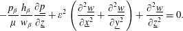
 $$\begin{eqnarray}\displaystyle & \displaystyle -\frac{p_{\unicode[STIX]{x1D6FD}}}{\unicode[STIX]{x1D707}}\frac{h_{\unicode[STIX]{x1D6FD}}^{2}}{u_{\unicode[STIX]{x1D6FD}}l_{\unicode[STIX]{x1D6FD}}}{\displaystyle \frac{\unicode[STIX]{x2202}\text{}\underline{p}}{\unicode[STIX]{x2202}\text{}\underline{x}}}+\unicode[STIX]{x1D700}^{2}\left({\displaystyle \frac{\unicode[STIX]{x2202}^{2}\text{}\underline{u}}{\unicode[STIX]{x2202}\text{}\underline{x}^{2}}}+{\displaystyle \frac{\unicode[STIX]{x2202}^{2}\text{}\underline{u}}{\unicode[STIX]{x2202}\text{}\underline{y}^{2}}}\right)+{\displaystyle \frac{\unicode[STIX]{x2202}^{2}\text{}\underline{u}}{\unicode[STIX]{x2202}\text{}\underline{z}^{2}}}=0, & \displaystyle\end{eqnarray}$$
 $$\begin{eqnarray}\displaystyle & \displaystyle -\frac{p_{\unicode[STIX]{x1D6FD}}}{\unicode[STIX]{x1D707}}\frac{h_{\unicode[STIX]{x1D6FD}}^{2}}{u_{\unicode[STIX]{x1D6FD}}l_{\unicode[STIX]{x1D6FD}}}{\displaystyle \frac{\unicode[STIX]{x2202}\text{}\underline{p}}{\unicode[STIX]{x2202}\text{}\underline{y}}}+\unicode[STIX]{x1D700}^{2}\left({\displaystyle \frac{\unicode[STIX]{x2202}^{2}\text{}\underline{v}}{\unicode[STIX]{x2202}\text{}\underline{x}^{2}}}+{\displaystyle \frac{\unicode[STIX]{x2202}^{2}\text{}\underline{v}}{\unicode[STIX]{x2202}\text{}\underline{y}^{2}}}\right)+{\displaystyle \frac{\unicode[STIX]{x2202}^{2}\text{}\underline{v}}{\unicode[STIX]{x2202}\text{}\underline{z}^{2}}}=0, & \displaystyle\end{eqnarray}$$
 $$\begin{eqnarray}\displaystyle & \displaystyle -\frac{p_{\unicode[STIX]{x1D6FD}}}{\unicode[STIX]{x1D707}}\frac{h_{\unicode[STIX]{x1D6FD}}}{w_{\unicode[STIX]{x1D6FD}}}{\displaystyle \frac{\unicode[STIX]{x2202}\text{}\underline{p}}{\unicode[STIX]{x2202}\text{}\underline{z}}}+\unicode[STIX]{x1D700}^{2}\left({\displaystyle \frac{\unicode[STIX]{x2202}^{2}\text{}\underline{w}}{\unicode[STIX]{x2202}\text{}\underline{x}^{2}}}+{\displaystyle \frac{\unicode[STIX]{x2202}^{2}\text{}\underline{w}}{\unicode[STIX]{x2202}\text{}\underline{y}^{2}}}\right)+{\displaystyle \frac{\unicode[STIX]{x2202}^{2}\text{}\underline{w}}{\unicode[STIX]{x2202}\text{}\underline{z}^{2}}}=0. & \displaystyle\end{eqnarray}$$
For least degeneracy, the characteristic pressure
 $p_{\unicode[STIX]{x1D6FD}}$
must be such that all the terms in (2.6a
) and (2.6b
) are of the same order of magnitude, and this is satisfied provided that
$p_{\unicode[STIX]{x1D6FD}}$
must be such that all the terms in (2.6a
) and (2.6b
) are of the same order of magnitude, and this is satisfied provided that
 $p_{\unicode[STIX]{x1D6FD}}=\unicode[STIX]{x1D707}u_{\unicode[STIX]{x1D6FD}}l_{\unicode[STIX]{x1D6FD}}/h_{\unicode[STIX]{x1D6FD}}^{2}$
. In this way, equations (2.6) can be rewritten as
$p_{\unicode[STIX]{x1D6FD}}=\unicode[STIX]{x1D707}u_{\unicode[STIX]{x1D6FD}}l_{\unicode[STIX]{x1D6FD}}/h_{\unicode[STIX]{x1D6FD}}^{2}$
. In this way, equations (2.6) can be rewritten as
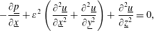 $$\begin{eqnarray}\displaystyle & \displaystyle -{\displaystyle \frac{\unicode[STIX]{x2202}\text{}\underline{p}}{\unicode[STIX]{x2202}\text{}\underline{x}}}+\unicode[STIX]{x1D700}^{2}\left({\displaystyle \frac{\unicode[STIX]{x2202}^{2}\text{}\underline{u}}{\unicode[STIX]{x2202}\text{}\underline{x}^{2}}}+{\displaystyle \frac{\unicode[STIX]{x2202}^{2}\text{}\underline{u}}{\unicode[STIX]{x2202}\text{}\underline{y}^{2}}}\right)+{\displaystyle \frac{\unicode[STIX]{x2202}^{2}\text{}\underline{u}}{\unicode[STIX]{x2202}\text{}\underline{z}^{2}}}=0, & \displaystyle\end{eqnarray}$$
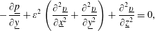 $$\begin{eqnarray}\displaystyle & \displaystyle -{\displaystyle \frac{\unicode[STIX]{x2202}\text{}\underline{p}}{\unicode[STIX]{x2202}\text{}\underline{y}}}+\unicode[STIX]{x1D700}^{2}\left({\displaystyle \frac{\unicode[STIX]{x2202}^{2}\text{}\underline{v}}{\unicode[STIX]{x2202}\text{}\underline{x}^{2}}}+{\displaystyle \frac{\unicode[STIX]{x2202}^{2}\text{}\underline{v}}{\unicode[STIX]{x2202}\text{}\underline{y}^{2}}}\right)+{\displaystyle \frac{\unicode[STIX]{x2202}^{2}\text{}\underline{v}}{\unicode[STIX]{x2202}\text{}\underline{z}^{2}}}=0, & \displaystyle\end{eqnarray}$$
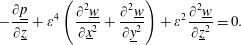 $$\begin{eqnarray}\displaystyle & \displaystyle -{\displaystyle \frac{\unicode[STIX]{x2202}\text{}\underline{p}}{\unicode[STIX]{x2202}\text{}\underline{z}}}+\unicode[STIX]{x1D700}^{4}\left({\displaystyle \frac{\unicode[STIX]{x2202}^{2}\text{}\underline{w}}{\unicode[STIX]{x2202}\text{}\underline{x}^{2}}}+{\displaystyle \frac{\unicode[STIX]{x2202}^{2}\text{}\underline{w}}{\unicode[STIX]{x2202}\text{}\underline{y}^{2}}}\right)+\unicode[STIX]{x1D700}^{2}{\displaystyle \frac{\unicode[STIX]{x2202}^{2}\text{}\underline{w}}{\unicode[STIX]{x2202}\text{}\underline{z}^{2}}}=0. & \displaystyle\end{eqnarray}$$
Using the fact that
 $\unicode[STIX]{x1D700}\ll 1$
, a truncation at
$\unicode[STIX]{x1D700}\ll 1$
, a truncation at
 $O(\unicode[STIX]{x1D700}^{2})$
yields the following form of the components of the momentum equation:
$O(\unicode[STIX]{x1D700}^{2})$
yields the following form of the components of the momentum equation:
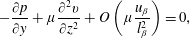
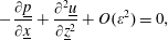 $$\begin{eqnarray}\displaystyle & \displaystyle -{\displaystyle \frac{\unicode[STIX]{x2202}\text{}\underline{p}}{\unicode[STIX]{x2202}\text{}\underline{x}}}+{\displaystyle \frac{\unicode[STIX]{x2202}^{2}\text{}\underline{u}}{\unicode[STIX]{x2202}\text{}\underline{z}^{2}}}+O(\unicode[STIX]{x1D700}^{2})=0, & \displaystyle\end{eqnarray}$$
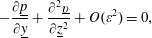 $$\begin{eqnarray}\displaystyle & \displaystyle -{\displaystyle \frac{\unicode[STIX]{x2202}\text{}\underline{p}}{\unicode[STIX]{x2202}\text{}\underline{y}}}+{\displaystyle \frac{\unicode[STIX]{x2202}^{2}\text{}\underline{v}}{\unicode[STIX]{x2202}\text{}\underline{z}^{2}}}+O(\unicode[STIX]{x1D700}^{2})=0, & \displaystyle\end{eqnarray}$$
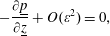 $$\begin{eqnarray}\displaystyle & \displaystyle -{\displaystyle \frac{\unicode[STIX]{x2202}\text{}\underline{p}}{\unicode[STIX]{x2202}\text{}\underline{z}}}+O(\unicode[STIX]{x1D700}^{2})=0, & \displaystyle\end{eqnarray}$$
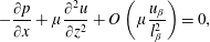 $$\begin{eqnarray}\displaystyle & \displaystyle -{\displaystyle \frac{\unicode[STIX]{x2202}p}{\unicode[STIX]{x2202}x}}+\unicode[STIX]{x1D707}{\displaystyle \frac{\unicode[STIX]{x2202}^{2}u}{\unicode[STIX]{x2202}z^{2}}}+O\left(\unicode[STIX]{x1D707}{\displaystyle \frac{u_{\unicode[STIX]{x1D6FD}}}{l_{\unicode[STIX]{x1D6FD}}^{2}}}\right)=0, & \displaystyle\end{eqnarray}$$
 $$\begin{eqnarray}\displaystyle & \displaystyle -{\displaystyle \frac{\unicode[STIX]{x2202}p}{\unicode[STIX]{x2202}y}}+\unicode[STIX]{x1D707}{\displaystyle \frac{\unicode[STIX]{x2202}^{2}v}{\unicode[STIX]{x2202}z^{2}}}+O\left(\unicode[STIX]{x1D707}{\displaystyle \frac{u_{\unicode[STIX]{x1D6FD}}}{l_{\unicode[STIX]{x1D6FD}}^{2}}}\right)=0, & \displaystyle\end{eqnarray}$$
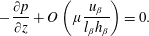 $$\begin{eqnarray}\displaystyle & \displaystyle -{\displaystyle \frac{\unicode[STIX]{x2202}p}{\unicode[STIX]{x2202}z}}+O\left(\unicode[STIX]{x1D707}{\displaystyle \frac{u_{\unicode[STIX]{x1D6FD}}}{l_{\unicode[STIX]{x1D6FD}}h_{\unicode[STIX]{x1D6FD}}}}\right)=0. & \displaystyle\end{eqnarray}$$
From (2.9c
), it can be seen that the pressure is independent of the
 $z$
coordinate. A double integration of (2.9a
) and (2.9b
) can thus be performed with respect to this coordinate, providing the two in-plane velocity profiles,
$z$
coordinate. A double integration of (2.9a
) and (2.9b
) can thus be performed with respect to this coordinate, providing the two in-plane velocity profiles,
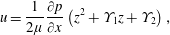 $$\begin{eqnarray}\displaystyle & \displaystyle u=\frac{1}{2\unicode[STIX]{x1D707}}{\displaystyle \frac{\unicode[STIX]{x2202}p}{\unicode[STIX]{x2202}x}}\left(z^{2}+\unicode[STIX]{x1D6F6}_{1}z+\unicode[STIX]{x1D6F6}_{2}\right), & \displaystyle\end{eqnarray}$$
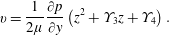 $$\begin{eqnarray}\displaystyle & \displaystyle v=\frac{1}{2\unicode[STIX]{x1D707}}{\displaystyle \frac{\unicode[STIX]{x2202}p}{\unicode[STIX]{x2202}y}}\left(z^{2}+\unicode[STIX]{x1D6F6}_{3}z+\unicode[STIX]{x1D6F6}_{4}\right). & \displaystyle\end{eqnarray}$$
In these equations,
 $\unicode[STIX]{x1D6F6}_{i}$
,
$\unicode[STIX]{x1D6F6}_{i}$
,
 $i=1,$
 $4$
, are four constants that need to be determined with the boundary condition in (2.1d
).
$4$
, are four constants that need to be determined with the boundary condition in (2.1d
).
2.2 Slip boundary condition
We now turn our attention to the first-order slip boundary condition in (2.1d
) with the purpose of a simplification consistent with an approximation at
 $O(\unicode[STIX]{x1D700}^{2})$
in accordance with the momentum balance equation. Denoting by
$O(\unicode[STIX]{x1D700}^{2})$
in accordance with the momentum balance equation. Denoting by
 $n_{xi}$
,
$n_{xi}$
,
 $n_{yi}$
and
$n_{yi}$
and
 $n_{zi}$
the
$n_{zi}$
the
 $x$
,
$x$
,
 $y$
and
$y$
and
 $z$
components of the normal unit vector
$z$
components of the normal unit vector
 $\boldsymbol{n}_{i}$
at the fracture wall
$\boldsymbol{n}_{i}$
at the fracture wall
 $z=h_{i}$
(
$z=h_{i}$
(
 $i=1$
,
$i=1$
,
 $2$
), where the velocity components are
$2$
), where the velocity components are
 $u_{i}$
,
$u_{i}$
,
 $v_{i}$
and
$v_{i}$
and
 $w_{i}$
, the general explicit form of (2.1d
) can be written as
$w_{i}$
, the general explicit form of (2.1d
) can be written as
 $$\begin{eqnarray}\displaystyle & \displaystyle u_{i}=-\unicode[STIX]{x1D709}\unicode[STIX]{x1D706}\left(A_{xi}\left(1-{n_{xi}}^{2}\right)-A_{yi}n_{xi}n_{yi}-A_{zi}n_{xi}n_{zi}\right), & \displaystyle\end{eqnarray}$$
 $$\begin{eqnarray}\displaystyle & \displaystyle v_{i}=-\unicode[STIX]{x1D709}\unicode[STIX]{x1D706}\left(-A_{xi}n_{xi}n_{yi}+A_{yi}\left(1-{n_{yi}}^{2}\right)-A_{zi}n_{yi}n_{zi}\right), & \displaystyle\end{eqnarray}$$
 $$\begin{eqnarray}\displaystyle & \displaystyle w_{i}=-\unicode[STIX]{x1D709}\unicode[STIX]{x1D706}\left(-A_{xi}n_{xi}n_{zi}-A_{yi}n_{yi}n_{zi}+A_{zi}\left(1-{n_{zi}}^{2}\right)\right). & \displaystyle\end{eqnarray}$$
 $A_{xi}$
,
$A_{xi}$
,
 $A_{yi}$
and
$A_{yi}$
and
 $A_{zi}$
are respectively defined as
$A_{zi}$
are respectively defined as 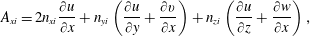 $$\begin{eqnarray}\displaystyle & \displaystyle A_{xi}=2n_{xi}{\displaystyle \frac{\unicode[STIX]{x2202}u}{\unicode[STIX]{x2202}x}}+n_{yi}\left({\displaystyle \frac{\unicode[STIX]{x2202}u}{\unicode[STIX]{x2202}y}}+{\displaystyle \frac{\unicode[STIX]{x2202}v}{\unicode[STIX]{x2202}x}}\right)+n_{zi}\left({\displaystyle \frac{\unicode[STIX]{x2202}u}{\unicode[STIX]{x2202}z}}+{\displaystyle \frac{\unicode[STIX]{x2202}w}{\unicode[STIX]{x2202}x}}\right), & \displaystyle\end{eqnarray}$$
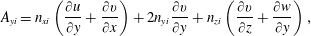 $$\begin{eqnarray}\displaystyle & \displaystyle A_{yi}=n_{xi}\left({\displaystyle \frac{\unicode[STIX]{x2202}u}{\unicode[STIX]{x2202}y}}+{\displaystyle \frac{\unicode[STIX]{x2202}v}{\unicode[STIX]{x2202}x}}\right)+2n_{yi}{\displaystyle \frac{\unicode[STIX]{x2202}v}{\unicode[STIX]{x2202}y}}+n_{zi}\left({\displaystyle \frac{\unicode[STIX]{x2202}v}{\unicode[STIX]{x2202}z}}+{\displaystyle \frac{\unicode[STIX]{x2202}w}{\unicode[STIX]{x2202}y}}\right), & \displaystyle\end{eqnarray}$$
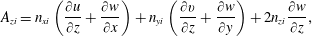 $$\begin{eqnarray}\displaystyle & \displaystyle A_{zi}=n_{xi}\left({\displaystyle \frac{\unicode[STIX]{x2202}u}{\unicode[STIX]{x2202}z}}+{\displaystyle \frac{\unicode[STIX]{x2202}w}{\unicode[STIX]{x2202}x}}\right)+n_{yi}\left({\displaystyle \frac{\unicode[STIX]{x2202}v}{\unicode[STIX]{x2202}z}}+{\displaystyle \frac{\unicode[STIX]{x2202}w}{\unicode[STIX]{x2202}y}}\right)+2n_{zi}{\displaystyle \frac{\unicode[STIX]{x2202}w}{\unicode[STIX]{x2202}z}}, & \displaystyle\end{eqnarray}$$
 $z=h_{i}$
(
$z=h_{i}$
(
 $i=1$
,
$i=1$
,
 $2$
) and where the components of
$2$
) and where the components of
 $\boldsymbol{n}_{i}$
are such that
$\boldsymbol{n}_{i}$
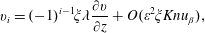
are such that 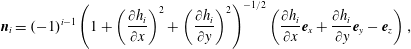 $$\begin{eqnarray}\boldsymbol{n}_{i}=(-1)^{i-1}\left(1+\left({\displaystyle \frac{\unicode[STIX]{x2202}h_{i}}{\unicode[STIX]{x2202}x}}\right)^{2}+\left({\displaystyle \frac{\unicode[STIX]{x2202}h_{i}}{\unicode[STIX]{x2202}y}}\right)^{2}\right)^{-1/2}\left({\displaystyle \frac{\unicode[STIX]{x2202}h_{i}}{\unicode[STIX]{x2202}x}}\boldsymbol{e}_{x}+{\displaystyle \frac{\unicode[STIX]{x2202}h_{i}}{\unicode[STIX]{x2202}y}}\boldsymbol{e}_{y}-\boldsymbol{e}_{z}\right),\end{eqnarray}$$
or, equivalently,
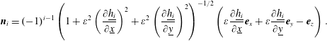 $$\begin{eqnarray}\boldsymbol{n}_{i}=(-1)^{i-1}\left(1+\unicode[STIX]{x1D700}^{2}\left({\displaystyle \frac{\unicode[STIX]{x2202}\text{}\underline{h_{i}}}{\unicode[STIX]{x2202}\text{}\underline{x}}}\right)^{2}+\unicode[STIX]{x1D700}^{2}\left({\displaystyle \frac{\unicode[STIX]{x2202}\text{}\underline{h_{i}}}{\unicode[STIX]{x2202}\text{}\underline{y}}}\right)^{2}\right)^{-1/2}\left(\unicode[STIX]{x1D700}{\displaystyle \frac{\unicode[STIX]{x2202}\text{}\underline{h_{i}}}{\unicode[STIX]{x2202}\text{}\underline{x}}}\boldsymbol{e}_{x}+\unicode[STIX]{x1D700}{\displaystyle \frac{\unicode[STIX]{x2202}\text{}\underline{h_{i}}}{\unicode[STIX]{x2202}\text{}\underline{y}}}\boldsymbol{e}_{y}-\boldsymbol{e}_{z}\right).\end{eqnarray}$$
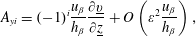
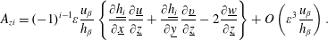
By inserting these expressions into (2.12), we obtain
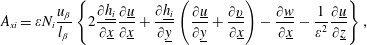 $$\begin{eqnarray}\displaystyle & \displaystyle A_{xi}=\unicode[STIX]{x1D700}N_{i}\frac{u_{\unicode[STIX]{x1D6FD}}}{l_{\unicode[STIX]{x1D6FD}}}\left\{2{\displaystyle \frac{\unicode[STIX]{x2202}\text{}\underline{h_{i}}}{\unicode[STIX]{x2202}\text{}\underline{x}}}{\displaystyle \frac{\unicode[STIX]{x2202}\text{}\underline{u}}{\unicode[STIX]{x2202}\text{}\underline{x}}}+{\displaystyle \frac{\unicode[STIX]{x2202}\text{}\underline{h_{i}}}{\unicode[STIX]{x2202}\text{}\underline{y}}}\left({\displaystyle \frac{\unicode[STIX]{x2202}\text{}\underline{u}}{\unicode[STIX]{x2202}\text{}\underline{y}}}+{\displaystyle \frac{\unicode[STIX]{x2202}\text{}\underline{v}}{\unicode[STIX]{x2202}\text{}\underline{x}}}\right)-{\displaystyle \frac{\unicode[STIX]{x2202}\text{}\underline{w}}{\unicode[STIX]{x2202}\text{}\underline{x}}}-\frac{1}{\unicode[STIX]{x1D700}^{2}}{\displaystyle \frac{\unicode[STIX]{x2202}\text{}\underline{u}}{\unicode[STIX]{x2202}\text{}\underline{z}}}\right\}, & \displaystyle\end{eqnarray}$$
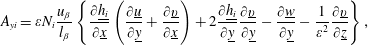 $$\begin{eqnarray}\displaystyle & \displaystyle A_{yi}=\unicode[STIX]{x1D700}N_{i}\frac{u_{\unicode[STIX]{x1D6FD}}}{l_{\unicode[STIX]{x1D6FD}}}\left\{{\displaystyle \frac{\unicode[STIX]{x2202}\text{}\underline{h_{i}}}{\unicode[STIX]{x2202}\text{}\underline{x}}}\left({\displaystyle \frac{\unicode[STIX]{x2202}\text{}\underline{u}}{\unicode[STIX]{x2202}\text{}\underline{y}}}+{\displaystyle \frac{\unicode[STIX]{x2202}\text{}\underline{v}}{\unicode[STIX]{x2202}\text{}\underline{x}}}\right)+2{\displaystyle \frac{\unicode[STIX]{x2202}\text{}\underline{h_{i}}}{\unicode[STIX]{x2202}\text{}\underline{y}}}{\displaystyle \frac{\unicode[STIX]{x2202}\text{}\underline{v}}{\unicode[STIX]{x2202}\text{}\underline{y}}}-{\displaystyle \frac{\unicode[STIX]{x2202}\text{}\underline{w}}{\unicode[STIX]{x2202}\text{}\underline{y}}}-\frac{1}{\unicode[STIX]{x1D700}^{2}}{\displaystyle \frac{\unicode[STIX]{x2202}\text{}\underline{v}}{\unicode[STIX]{x2202}\text{}\underline{z}}}\right\}, & \displaystyle\end{eqnarray}$$
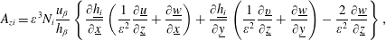 $$\begin{eqnarray}\displaystyle & \displaystyle A_{zi}=\unicode[STIX]{x1D700}^{3}N_{i}\frac{u_{\unicode[STIX]{x1D6FD}}}{h_{\unicode[STIX]{x1D6FD}}}\left\{{\displaystyle \frac{\unicode[STIX]{x2202}\text{}\underline{h_{i}}}{\unicode[STIX]{x2202}\text{}\underline{x}}}\left(\frac{1}{\unicode[STIX]{x1D700}^{2}}{\displaystyle \frac{\unicode[STIX]{x2202}\text{}\underline{u}}{\unicode[STIX]{x2202}\text{}\underline{z}}}+{\displaystyle \frac{\unicode[STIX]{x2202}\text{}\underline{w}}{\unicode[STIX]{x2202}\text{}\underline{x}}}\right)+{\displaystyle \frac{\unicode[STIX]{x2202}\text{}\underline{h_{i}}}{\unicode[STIX]{x2202}\text{}\underline{y}}}\left(\frac{1}{\unicode[STIX]{x1D700}^{2}}{\displaystyle \frac{\unicode[STIX]{x2202}\text{}\underline{v}}{\unicode[STIX]{x2202}\text{}\underline{z}}}+{\displaystyle \frac{\unicode[STIX]{x2202}\text{}\underline{w}}{\unicode[STIX]{x2202}\text{}\underline{y}}}\right)-\frac{2}{\unicode[STIX]{x1D700}^{2}}{\displaystyle \frac{\unicode[STIX]{x2202}\text{}\underline{w}}{\unicode[STIX]{x2202}\text{}\underline{z}}}\right\}, & \displaystyle\end{eqnarray}$$
 $N_{i}=(-1)^{i-1}(1+\unicode[STIX]{x1D700}^{2}(\unicode[STIX]{x2202}\text{}\underline{h_{i}}/\unicode[STIX]{x2202}\text{}\underline{x})^{2}+\unicode[STIX]{x1D700}^{2}(\unicode[STIX]{x2202}\text{}\underline{h_{i}}/\unicode[STIX]{x2202}\text{}\underline{y})^{2})^{-1/2}$
. Since
$N_{i}=(-1)^{i-1}(1+\unicode[STIX]{x1D700}^{2}(\unicode[STIX]{x2202}\text{}\underline{h_{i}}/\unicode[STIX]{x2202}\text{}\underline{x})^{2}+\unicode[STIX]{x1D700}^{2}(\unicode[STIX]{x2202}\text{}\underline{h_{i}}/\unicode[STIX]{x2202}\text{}\underline{y})^{2})^{-1/2}$
. Since
 $\unicode[STIX]{x1D700}\ll 1$
,
$\unicode[STIX]{x1D700}\ll 1$
,
 $N_{i}=(-1)^{i-1}+O(\unicode[STIX]{x1D700}^{2})$
, so that, at
$N_{i}=(-1)^{i-1}+O(\unicode[STIX]{x1D700}^{2})$
, so that, at
 $O(\unicode[STIX]{x1D700}^{2})$
, equations (2.15) can be simplified to give
$O(\unicode[STIX]{x1D700}^{2})$
, equations (2.15) can be simplified to give 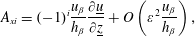 $$\begin{eqnarray}\displaystyle & \displaystyle A_{xi}=(-1)^{i}\frac{u_{\unicode[STIX]{x1D6FD}}}{h_{\unicode[STIX]{x1D6FD}}}{\displaystyle \frac{\unicode[STIX]{x2202}\text{}\underline{u}}{\unicode[STIX]{x2202}\text{}\underline{z}}}+O\left(\unicode[STIX]{x1D700}^{2}\frac{u_{\unicode[STIX]{x1D6FD}}}{h_{\unicode[STIX]{x1D6FD}}}\right), & \displaystyle\end{eqnarray}$$
 $$\begin{eqnarray}\displaystyle & \displaystyle A_{yi}=(-1)^{i}\frac{u_{\unicode[STIX]{x1D6FD}}}{h_{\unicode[STIX]{x1D6FD}}}{\displaystyle \frac{\unicode[STIX]{x2202}\text{}\underline{v}}{\unicode[STIX]{x2202}\text{}\underline{z}}}+O\left(\unicode[STIX]{x1D700}^{2}\frac{u_{\unicode[STIX]{x1D6FD}}}{h_{\unicode[STIX]{x1D6FD}}}\right), & \displaystyle\end{eqnarray}$$
 $$\begin{eqnarray}\displaystyle & \displaystyle A_{zi}=(-1)^{i-1}\unicode[STIX]{x1D700}\frac{u_{\unicode[STIX]{x1D6FD}}}{h_{\unicode[STIX]{x1D6FD}}}\left\{{\displaystyle \frac{\unicode[STIX]{x2202}\text{}\underline{h_{i}}}{\unicode[STIX]{x2202}\text{}\underline{x}}}{\displaystyle \frac{\unicode[STIX]{x2202}\text{}\underline{u}}{\unicode[STIX]{x2202}\text{}\underline{z}}}+{\displaystyle \frac{\unicode[STIX]{x2202}\text{}\underline{h_{i}}}{\unicode[STIX]{x2202}\text{}\underline{y}}}{\displaystyle \frac{\unicode[STIX]{x2202}\text{}\underline{v}}{\unicode[STIX]{x2202}\text{}\underline{z}}}-2{\displaystyle \frac{\unicode[STIX]{x2202}\text{}\underline{w}}{\unicode[STIX]{x2202}\text{}\underline{z}}}\right\}+O\left(\unicode[STIX]{x1D700}^{3}\frac{u_{\unicode[STIX]{x1D6FD}}}{h_{\unicode[STIX]{x1D6FD}}}\right). & \displaystyle\end{eqnarray}$$
Once reported in (2.11), the dimensionless slip velocity components at
 $z=h_{i}$
can hence be approximated at
$z=h_{i}$
can hence be approximated at
 $O(\unicode[STIX]{x1D700}^{2}\unicode[STIX]{x1D709}Kn)$
by
$O(\unicode[STIX]{x1D700}^{2}\unicode[STIX]{x1D709}Kn)$
by
 $$\begin{eqnarray}\displaystyle & \displaystyle \text{}\underline{u_{i}}=(-1)^{i-1}\unicode[STIX]{x1D709}Kn{\displaystyle \frac{\unicode[STIX]{x2202}\text{}\underline{u}}{\unicode[STIX]{x2202}\text{}\underline{z}}}+O(\unicode[STIX]{x1D700}^{2}\unicode[STIX]{x1D709}Kn), & \displaystyle\end{eqnarray}$$
 $$\begin{eqnarray}\displaystyle & \displaystyle \text{}\underline{v_{i}}=(-1)^{i-1}\unicode[STIX]{x1D709}Kn{\displaystyle \frac{\unicode[STIX]{x2202}\text{}\underline{v}}{\unicode[STIX]{x2202}\text{}\underline{z}}}+O(\unicode[STIX]{x1D700}^{2}\unicode[STIX]{x1D709}Kn), & \displaystyle\end{eqnarray}$$
 $$\begin{eqnarray}\displaystyle & \displaystyle \text{}\underline{w_{i}}=(-1)^{i-1}\unicode[STIX]{x1D709}Kn\left({\displaystyle \frac{\unicode[STIX]{x2202}\text{}\underline{h_{i}}}{\unicode[STIX]{x2202}\text{}\underline{x}}}{\displaystyle \frac{\unicode[STIX]{x2202}\text{}\underline{u}}{\unicode[STIX]{x2202}\text{}\underline{z}}}+{\displaystyle \frac{\unicode[STIX]{x2202}\text{}\underline{h_{i}}}{\unicode[STIX]{x2202}\text{}\underline{y}}}{\displaystyle \frac{\unicode[STIX]{x2202}\text{}\underline{v}}{\unicode[STIX]{x2202}\text{}\underline{z}}}\right)+O(\unicode[STIX]{x1D700}^{2}\unicode[STIX]{x1D709}Kn), & \displaystyle\end{eqnarray}$$
 $Kn$
denotes the Knudsen number, defined by
$Kn$
denotes the Knudsen number, defined by  $$\begin{eqnarray}Kn=\unicode[STIX]{x1D706}/h_{\unicode[STIX]{x1D6FD}}.\end{eqnarray}$$
It must be noted that, due to the fact that
 $\unicode[STIX]{x1D709}Kn$
remains smaller than unity in the context of slip flow, this approximation is consistent with that derived so far at
$\unicode[STIX]{x1D709}Kn$
remains smaller than unity in the context of slip flow, this approximation is consistent with that derived so far at
 $O(\unicode[STIX]{x1D700}^{2})$
.
$O(\unicode[STIX]{x1D700}^{2})$
.
In the dimensional form, this yields, at
 $z=h_{i}$
(
$z=h_{i}$
(
 $i=1,2$
),
$i=1,2$
),
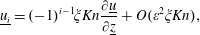
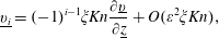
 $$\begin{eqnarray}\displaystyle & \displaystyle u_{i}=(-1)^{i-1}\unicode[STIX]{x1D709}\unicode[STIX]{x1D706}{\displaystyle \frac{\unicode[STIX]{x2202}u}{\unicode[STIX]{x2202}z}}+O(\unicode[STIX]{x1D700}^{2}\unicode[STIX]{x1D709}Knu_{\unicode[STIX]{x1D6FD}}), & \displaystyle\end{eqnarray}$$
 $$\begin{eqnarray}\displaystyle & \displaystyle v_{i}=(-1)^{i-1}\unicode[STIX]{x1D709}\unicode[STIX]{x1D706}{\displaystyle \frac{\unicode[STIX]{x2202}v}{\unicode[STIX]{x2202}z}}+O(\unicode[STIX]{x1D700}^{2}\unicode[STIX]{x1D709}Knu_{\unicode[STIX]{x1D6FD}}), & \displaystyle\end{eqnarray}$$
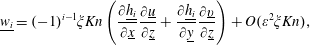
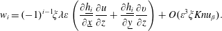 $$\begin{eqnarray}\displaystyle & \displaystyle w_{i}=(-1)^{i-1}\unicode[STIX]{x1D709}\unicode[STIX]{x1D706}\unicode[STIX]{x1D700}\left({\displaystyle \frac{\unicode[STIX]{x2202}\text{}\underline{h_{i}}}{\unicode[STIX]{x2202}\text{}\underline{x}}}{\displaystyle \frac{\unicode[STIX]{x2202}u}{\unicode[STIX]{x2202}z}}+{\displaystyle \frac{\unicode[STIX]{x2202}\text{}\underline{h_{i}}}{\unicode[STIX]{x2202}\text{}\underline{y}}}{\displaystyle \frac{\unicode[STIX]{x2202}v}{\unicode[STIX]{x2202}z}}\right)+O(\unicode[STIX]{x1D700}^{3}\unicode[STIX]{x1D709}Knu_{\unicode[STIX]{x1D6FD}}). & \displaystyle\end{eqnarray}$$
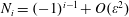
As expected, equation (2.19c
) clearly indicates that the vertical velocity
 $w_{i}$
is smaller than the in-plane velocities
$w_{i}$
is smaller than the in-plane velocities
 $u_{i}$
and
$u_{i}$
and
 $v_{i}$
(
$v_{i}$
(
 $i=1,2$
) by a factor
$i=1,2$
) by a factor
 $\unicode[STIX]{x1D700}$
. Under the small-slope hypothesis, the first-order boundary condition (2.1d
) simplifies to equations (2.19) at the bottom and top surfaces, and this justifies the form put forth without formal demonstration by Burgdorfer (Reference Burgdorfer1959) in a study of gas lubricated bearings.
$\unicode[STIX]{x1D700}$
. Under the small-slope hypothesis, the first-order boundary condition (2.1d
) simplifies to equations (2.19) at the bottom and top surfaces, and this justifies the form put forth without formal demonstration by Burgdorfer (Reference Burgdorfer1959) in a study of gas lubricated bearings.
2.3 Local Reynolds equation
To complete the flow solution, the constants of integration
 $\unicode[STIX]{x1D6F6}_{i}$
(
$\unicode[STIX]{x1D6F6}_{i}$
(
 $i=1,4$
) in (2.10) may be determined by making use of the relationships in (2.19a
) and (2.19b
). Solution of the system of equations for
$i=1,4$
) in (2.10) may be determined by making use of the relationships in (2.19a
) and (2.19b
). Solution of the system of equations for
 $\unicode[STIX]{x1D6F6}_{i}$
yields the expressions of the in-plane parabolic velocity profiles,
$\unicode[STIX]{x1D6F6}_{i}$
yields the expressions of the in-plane parabolic velocity profiles,
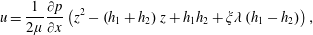 $$\begin{eqnarray}\displaystyle & \displaystyle u=\frac{1}{2\unicode[STIX]{x1D707}}{\displaystyle \frac{\unicode[STIX]{x2202}p}{\unicode[STIX]{x2202}x}}\left(z^{2}-\left(h_{1}+h_{2}\right)z+h_{1}h_{2}+\unicode[STIX]{x1D709}\unicode[STIX]{x1D706}\left(h_{1}-h_{2}\right)\right), & \displaystyle\end{eqnarray}$$
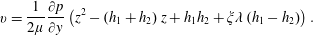 $$\begin{eqnarray}\displaystyle & \displaystyle v=\frac{1}{2\unicode[STIX]{x1D707}}{\displaystyle \frac{\unicode[STIX]{x2202}p}{\unicode[STIX]{x2202}y}}\left(z^{2}-\left(h_{1}+h_{2}\right)z+h_{1}h_{2}+\unicode[STIX]{x1D709}\unicode[STIX]{x1D706}\left(h_{1}-h_{2}\right)\right). & \displaystyle\end{eqnarray}$$
At this point, the aim is to reduce the flow model from its original 3D form to an equivalent 2D version that is
 $O(\unicode[STIX]{x1D700}^{2}\unicode[STIX]{x1D709}Kn)$
. Recalling that the fluid is considered as barotropic (see (2.1c
)) and that the pressure is independent of the
$O(\unicode[STIX]{x1D700}^{2}\unicode[STIX]{x1D709}Kn)$
. Recalling that the fluid is considered as barotropic (see (2.1c
)) and that the pressure is independent of the
 $z$
coordinate (see (2.9c
)), the mass flow rate per unit width of the fracture can be obtained by integrating the mass flux across the aperture, which gives
$z$
coordinate (see (2.9c
)), the mass flow rate per unit width of the fracture can be obtained by integrating the mass flux across the aperture, which gives
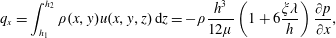 $$\begin{eqnarray}\displaystyle & \displaystyle q_{x}=\int _{h_{1}}^{h_{2}}\unicode[STIX]{x1D70C}(x,y)u(x,y,z)\,\text{d}z=-\unicode[STIX]{x1D70C}\frac{h^{3}}{12\unicode[STIX]{x1D707}}\left(1+6\frac{\unicode[STIX]{x1D709}\unicode[STIX]{x1D706}}{h}\right){\displaystyle \frac{\unicode[STIX]{x2202}p}{\unicode[STIX]{x2202}x}}, & \displaystyle\end{eqnarray}$$
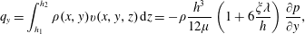 $$\begin{eqnarray}\displaystyle & \displaystyle q_{y}=\int _{h_{1}}^{h_{2}}\unicode[STIX]{x1D70C}(x,y)v(x,y,z)\,\text{d}z=-\unicode[STIX]{x1D70C}\frac{h^{3}}{12\unicode[STIX]{x1D707}}\left(1+6\frac{\unicode[STIX]{x1D709}\unicode[STIX]{x1D706}}{h}\right){\displaystyle \frac{\unicode[STIX]{x2202}p}{\unicode[STIX]{x2202}y}}, & \displaystyle\end{eqnarray}$$
 $h=h_{2}-h_{1}$
. Letting
$h=h_{2}-h_{1}$
. Letting
 $\boldsymbol{q}=q_{x}\boldsymbol{e}_{\boldsymbol{x}}+q_{y}\boldsymbol{e}_{\boldsymbol{y}}$
, this can be written in a vectorial 2D form as
$\boldsymbol{q}=q_{x}\boldsymbol{e}_{\boldsymbol{x}}+q_{y}\boldsymbol{e}_{\boldsymbol{y}}$
, this can be written in a vectorial 2D form as 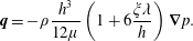 $$\begin{eqnarray}\boldsymbol{q}=-\unicode[STIX]{x1D70C}\frac{h^{3}}{12\unicode[STIX]{x1D707}}\left(1+6\frac{\unicode[STIX]{x1D709}\unicode[STIX]{x1D706}}{h}\right)\unicode[STIX]{x1D735}p.\end{eqnarray}$$
The continuity equation (2.1a
) can also be integrated in the
 $z$
-direction across the aperture to give
$z$
-direction across the aperture to give
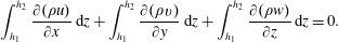 $$\begin{eqnarray}\int _{h_{1}}^{h_{2}}{\displaystyle \frac{\unicode[STIX]{x2202}(\unicode[STIX]{x1D70C}u)}{\unicode[STIX]{x2202}x}}\,\text{d}z+\int _{h_{1}}^{h_{2}}{\displaystyle \frac{\unicode[STIX]{x2202}(\unicode[STIX]{x1D70C}v)}{\unicode[STIX]{x2202}y}}\,\text{d}z+\int _{h_{1}}^{h_{2}}{\displaystyle \frac{\unicode[STIX]{x2202}(\unicode[STIX]{x1D70C}w)}{\unicode[STIX]{x2202}z}}\,\text{d}z=0.\end{eqnarray}$$
Using the definition of the mass flow rate per unit fracture width used in (2.21) and the Leibniz rule, one obtains
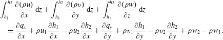 $$\begin{eqnarray}\displaystyle & & \displaystyle \int _{h_{1}}^{h_{2}}{\displaystyle \frac{\unicode[STIX]{x2202}(\unicode[STIX]{x1D70C}u)}{\unicode[STIX]{x2202}x}}\,\text{d}z+\int _{h_{1}}^{h_{2}}{\displaystyle \frac{\unicode[STIX]{x2202}(\unicode[STIX]{x1D70C}v)}{\unicode[STIX]{x2202}y}}\,\text{d}z+\int _{h_{1}}^{h_{2}}{\displaystyle \frac{\unicode[STIX]{x2202}(\unicode[STIX]{x1D70C}w)}{\unicode[STIX]{x2202}z}}\,\text{d}z\nonumber\\ \displaystyle & & \displaystyle \quad ={\displaystyle \frac{\unicode[STIX]{x2202}q_{x}}{\unicode[STIX]{x2202}x}}+\unicode[STIX]{x1D70C}u_{1}{\displaystyle \frac{\unicode[STIX]{x2202}h_{1}}{\unicode[STIX]{x2202}x}}-\unicode[STIX]{x1D70C}u_{2}{\displaystyle \frac{\unicode[STIX]{x2202}h_{2}}{\unicode[STIX]{x2202}x}}+{\displaystyle \frac{\unicode[STIX]{x2202}q_{y}}{\unicode[STIX]{x2202}y}}+\unicode[STIX]{x1D70C}v_{1}{\displaystyle \frac{\unicode[STIX]{x2202}h_{1}}{\unicode[STIX]{x2202}y}}-\unicode[STIX]{x1D70C}v_{2}{\displaystyle \frac{\unicode[STIX]{x2202}h_{2}}{\unicode[STIX]{x2202}y}}+\unicode[STIX]{x1D70C}w_{2}-\unicode[STIX]{x1D70C}w_{1}.\end{eqnarray}$$
This can be written in a more compact form as (we use Einstein’s notation)
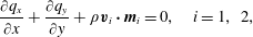 $$\begin{eqnarray}{\displaystyle \frac{\unicode[STIX]{x2202}q_{x}}{\unicode[STIX]{x2202}x}}+{\displaystyle \frac{\unicode[STIX]{x2202}q_{y}}{\unicode[STIX]{x2202}y}}+\unicode[STIX]{x1D70C}\boldsymbol{v}_{i}\boldsymbol{\cdot }\boldsymbol{m}_{i}=0,\quad i=1,~2,\end{eqnarray}$$
where
 $$\begin{eqnarray}\boldsymbol{v}_{i}=u_{i}\boldsymbol{e}_{x}+v_{i}\boldsymbol{e}_{y}+w_{i}\boldsymbol{e}_{z},\quad \boldsymbol{m}_{i}=\left(-1\right)^{i-1}\left({\displaystyle \frac{\unicode[STIX]{x2202}h_{i}}{\unicode[STIX]{x2202}x}}\boldsymbol{e}_{x}+{\displaystyle \frac{\unicode[STIX]{x2202}h_{i}}{\unicode[STIX]{x2202}y}}\boldsymbol{e}_{y}-\boldsymbol{e}_{z}\right),\quad i=1,~2.\end{eqnarray}$$
Because
 $\boldsymbol{v}_{i}$
is tangential at the surface
$\boldsymbol{v}_{i}$
is tangential at the surface
 $z=h_{i}$
(
$z=h_{i}$
(
 $i=1,2$
) while
$i=1,2$
) while
 $\boldsymbol{m}_{i}$
is proportional to the normal vector
$\boldsymbol{m}_{i}$
is proportional to the normal vector
 $\boldsymbol{n}_{i}$
at this surface (see (2.13)), the integrated mass conservation equation (2.23) reduces to
$\boldsymbol{n}_{i}$
at this surface (see (2.13)), the integrated mass conservation equation (2.23) reduces to
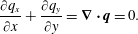 $$\begin{eqnarray}{\displaystyle \frac{\unicode[STIX]{x2202}q_{x}}{\unicode[STIX]{x2202}x}}+{\displaystyle \frac{\unicode[STIX]{x2202}q_{y}}{\unicode[STIX]{x2202}y}}=\unicode[STIX]{x1D735}\boldsymbol{\cdot }\boldsymbol{q}=0.\end{eqnarray}$$
This result is exact at any order of
 $\unicode[STIX]{x1D700}$
and
$\unicode[STIX]{x1D700}$
and
 $\unicode[STIX]{x1D709}Kn$
as it was directly derived from (2.1d
). The same result could have been obtained at
$\unicode[STIX]{x1D709}Kn$
as it was directly derived from (2.1d
). The same result could have been obtained at
 $O(\unicode[STIX]{x1D700}^{2}\unicode[STIX]{x1D709}Kn)$
by replacing (2.19) in (2.24).
$O(\unicode[STIX]{x1D700}^{2}\unicode[STIX]{x1D709}Kn)$
by replacing (2.19) in (2.24).
The original boundary-value problem (2.1) is now reduced from a 3D form to a 2D one in the
 $(x,y)$
plane. If
$(x,y)$
plane. If
 ${\mathcal{A}}_{\unicode[STIX]{x1D6FD}}$
designates the 2D region occupied by the fluid phase and
${\mathcal{A}}_{\unicode[STIX]{x1D6FD}}$
designates the 2D region occupied by the fluid phase and
 ${\mathcal{A}}_{\unicode[STIX]{x1D70E}}$
the 2D region corresponding to the solid phase, i.e. the contact zones, the flow problem in (2.1) can be equivalently formulated in the following version, which is second-order-accurate in the local slope of the wall roughness and first-order-accurate in the Knudsen number, as
${\mathcal{A}}_{\unicode[STIX]{x1D70E}}$
the 2D region corresponding to the solid phase, i.e. the contact zones, the flow problem in (2.1) can be equivalently formulated in the following version, which is second-order-accurate in the local slope of the wall roughness and first-order-accurate in the Knudsen number, as
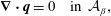 $$\begin{eqnarray}\displaystyle & \displaystyle \unicode[STIX]{x1D735}\boldsymbol{\cdot }\boldsymbol{q}=0\quad \text{in }{\mathcal{A}}_{\unicode[STIX]{x1D6FD}}, & \displaystyle\end{eqnarray}$$
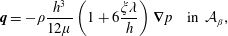 $$\begin{eqnarray}\displaystyle & \displaystyle \boldsymbol{q}=-\unicode[STIX]{x1D70C}\frac{h^{3}}{12\unicode[STIX]{x1D707}}\left(1+6\frac{\unicode[STIX]{x1D709}\unicode[STIX]{x1D706}}{h}\right)\unicode[STIX]{x1D735}p\quad \text{in }{\mathcal{A}}_{\unicode[STIX]{x1D6FD}}, & \displaystyle\end{eqnarray}$$
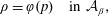 $$\begin{eqnarray}\displaystyle & \displaystyle \unicode[STIX]{x1D70C}=\unicode[STIX]{x1D711}(p)\quad \text{in }{\mathcal{A}}_{\unicode[STIX]{x1D6FD}}, & \displaystyle\end{eqnarray}$$
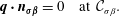 $$\begin{eqnarray}\displaystyle & \displaystyle \boldsymbol{q}\boldsymbol{\cdot }\boldsymbol{n}_{\unicode[STIX]{x1D748}\unicode[STIX]{x1D737}}=0\quad \text{at }{\mathcal{C}}_{\unicode[STIX]{x1D70E}\unicode[STIX]{x1D6FD}}. & \displaystyle\end{eqnarray}$$
 $\boldsymbol{n}_{\unicode[STIX]{x1D748}\unicode[STIX]{x1D737}}$
is the normal unit vector to the contours
$\boldsymbol{n}_{\unicode[STIX]{x1D748}\unicode[STIX]{x1D737}}$
is the normal unit vector to the contours
 ${\mathcal{C}}_{\unicode[STIX]{x1D70E}\unicode[STIX]{x1D6FD}}$
of
${\mathcal{C}}_{\unicode[STIX]{x1D70E}\unicode[STIX]{x1D6FD}}$
of
 ${\mathcal{A}}_{\unicode[STIX]{x1D70E}}$
in the (
${\mathcal{A}}_{\unicode[STIX]{x1D70E}}$
in the (
 $\boldsymbol{e}_{x},~\boldsymbol{e}_{y}$
) plane, pointing from the fluid phase towards the solid phase. This boundary condition refers to the impermeability of the contact zones when they exist.
$\boldsymbol{e}_{x},~\boldsymbol{e}_{y}$
) plane, pointing from the fluid phase towards the solid phase. This boundary condition refers to the impermeability of the contact zones when they exist. Equations (2.28b
) and (2.28a
) form the Reynolds model of a pressure-driven slip flow. The local transmissivity is identified as
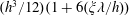 $(h^{3}/12)(1+6(\unicode[STIX]{x1D709}\unicode[STIX]{x1D706}/h))$
, where the second term in the parentheses reflects the correction for slip flow in which
$(h^{3}/12)(1+6(\unicode[STIX]{x1D709}\unicode[STIX]{x1D706}/h))$
, where the second term in the parentheses reflects the correction for slip flow in which
 $\unicode[STIX]{x1D706}/h$
can be viewed as the local Knudsen number. This term vanishes to obtain the Reynolds flow model with a classical local transmissivity
$\unicode[STIX]{x1D706}/h$
can be viewed as the local Knudsen number. This term vanishes to obtain the Reynolds flow model with a classical local transmissivity
 $h^{3}/12$
for a slightly compressible or incompressible flow in the absence of slip at the solid–fluid interfaces (Szeri Reference Szeri1998; Vallet et al.
Reference Vallet, Lasseux, Sainsot and Zahouani2009).
$h^{3}/12$
for a slightly compressible or incompressible flow in the absence of slip at the solid–fluid interfaces (Szeri Reference Szeri1998; Vallet et al.
Reference Vallet, Lasseux, Sainsot and Zahouani2009).
3 Upscaling of the Reynolds flow model
The boundary-value problem (2.28) describes the viscous slip flow at the roughness scale. The interest is now to derive a macroscopic flow model that relates the macroscopic mass flow rate per unit width at the scale of a representative elementary surface (RES) to the macroscopic pressure gradient. To do so, we make use of a formalism completely similar to the volume averaging method (Whitaker Reference Whitaker1999). Averaging is performed over a domain
 ${\mathcal{S}}$
of surface
${\mathcal{S}}$
of surface
 $S$
and radius
$S$
and radius
 $r_{0}$
that is a sample of the entire fracture of dimension
$r_{0}$
that is a sample of the entire fracture of dimension
 $L_{0}$
, as shown in figure 2. The fluid phase
$L_{0}$
, as shown in figure 2. The fluid phase
 $\unicode[STIX]{x1D6FD}$
within this averaging domain occupies a region
$\unicode[STIX]{x1D6FD}$
within this averaging domain occupies a region
 ${\mathcal{S}}_{\unicode[STIX]{x1D6FD}}$
of surface
${\mathcal{S}}_{\unicode[STIX]{x1D6FD}}$
of surface
 $S_{\unicode[STIX]{x1D6FD}}$
. For any given quantity
$S_{\unicode[STIX]{x1D6FD}}$
. For any given quantity
 $\unicode[STIX]{x1D713}$
defined in
$\unicode[STIX]{x1D713}$
defined in
 ${\mathcal{S}}_{\unicode[STIX]{x1D6FD}}$
, two distinct averages may be used (Whitaker Reference Whitaker1999), namely the superficial average, which can be expressed as
${\mathcal{S}}_{\unicode[STIX]{x1D6FD}}$
, two distinct averages may be used (Whitaker Reference Whitaker1999), namely the superficial average, which can be expressed as
 $$\begin{eqnarray}\langle \unicode[STIX]{x1D713}\rangle ={\displaystyle \frac{1}{S}}\int _{{\mathcal{S}}_{\unicode[STIX]{x1D6FD}}}^{}\unicode[STIX]{x1D713}\,\text{d}S,\end{eqnarray}$$
and the intrinsic average, which is defined by
 $$\begin{eqnarray}\langle \unicode[STIX]{x1D713}\rangle ^{\unicode[STIX]{x1D6FD}}={\displaystyle \frac{1}{S_{\unicode[STIX]{x1D6FD}}}}\int _{{\mathcal{S}}_{\unicode[STIX]{x1D6FD}}}^{}\unicode[STIX]{x1D713}\,\text{d}S.\end{eqnarray}$$
When the superficial average is applied to the problem given by (2.28) with the purpose of obtaining a macroscopic model involving averaged quantities only, spatial differentiation and averaging operators need to be inverted. This is achieved by making use of the spatial averaging theorem, a special form of the Leibniz rule, which, for the gradient of a scalar quantity, yields (Howes & Whitaker Reference Howes and Whitaker1985)
 $$\begin{eqnarray}\langle \unicode[STIX]{x1D735}\unicode[STIX]{x1D713}\rangle =\unicode[STIX]{x1D735}\langle \unicode[STIX]{x1D713}\rangle +{\displaystyle \frac{1}{S}}\int _{{\mathcal{C}}_{\unicode[STIX]{x1D70E}\unicode[STIX]{x1D6FD}}}^{}\unicode[STIX]{x1D713}\boldsymbol{n}_{\unicode[STIX]{x1D748}\unicode[STIX]{x1D737}}\,\text{d}l\end{eqnarray}$$
and a similar version for the divergence operator.
As for any upscaling process, the development of the macroscopic model relies on the hypothesis of a scale separation, namely
 $$\begin{eqnarray}l_{\unicode[STIX]{x1D6FD}}\ll r_{0}\ll L_{0}.\end{eqnarray}$$
The scale
 $L_{0}$
in the above relationship is used, for the sake of simplicity in the presentation, as the scale of the fracture itself, while assuming that it remains homogeneous, i.e. that no other scale is involved in the flow process. This is not always the case in practice, and to be more precise,
$L_{0}$
in the above relationship is used, for the sake of simplicity in the presentation, as the scale of the fracture itself, while assuming that it remains homogeneous, i.e. that no other scale is involved in the flow process. This is not always the case in practice, and to be more precise,
 $L_{0}$
should be understood as the length scale of defaults of characteristic size immediately larger than
$L_{0}$
should be understood as the length scale of defaults of characteristic size immediately larger than
 $l_{\unicode[STIX]{x1D6FD}}$
. In the remainder of this article, this hierarchy expressed in (3.4) is assumed, a constraint that is usually not too difficult to satisfy, except maybe for some fracture patterns in natural geological media. Under these circumstances, a spatial decomposition on
$l_{\unicode[STIX]{x1D6FD}}$
. In the remainder of this article, this hierarchy expressed in (3.4) is assumed, a constraint that is usually not too difficult to satisfy, except maybe for some fracture patterns in natural geological media. Under these circumstances, a spatial decomposition on
 $\unicode[STIX]{x1D713}$
can be performed according to (Gray Reference Gray1975)
$\unicode[STIX]{x1D713}$
can be performed according to (Gray Reference Gray1975)
 $$\begin{eqnarray}\unicode[STIX]{x1D713}=\langle \unicode[STIX]{x1D713}\rangle ^{\unicode[STIX]{x1D6FD}}+\widetilde{\unicode[STIX]{x1D713}}.\end{eqnarray}$$
The quantity
 $\widetilde{\unicode[STIX]{x1D713}}$
refers to the spatial deviation of
$\widetilde{\unicode[STIX]{x1D713}}$
refers to the spatial deviation of
 $\unicode[STIX]{x1D713}$
from its average value and has a length scale of variation
$\unicode[STIX]{x1D713}$
from its average value and has a length scale of variation
 $l_{\unicode[STIX]{x1D6FD}}$
(i.e. the roughness scale), while the characteristic length scale of variation for the average quantity
$l_{\unicode[STIX]{x1D6FD}}$
(i.e. the roughness scale), while the characteristic length scale of variation for the average quantity
 $\langle \unicode[STIX]{x1D713}\rangle ^{\unicode[STIX]{x1D6FD}}$
is of the order of
$\langle \unicode[STIX]{x1D713}\rangle ^{\unicode[STIX]{x1D6FD}}$
is of the order of
 $L_{0}$
(see figure 2). If the scale hierarchy expressed in (3.4) is fulfilled, it can be shown (Whitaker Reference Whitaker1999) that the intrinsic average exhibits negligible variations within the RES, which means that
$L_{0}$
(see figure 2). If the scale hierarchy expressed in (3.4) is fulfilled, it can be shown (Whitaker Reference Whitaker1999) that the intrinsic average exhibits negligible variations within the RES, which means that
 $$\begin{eqnarray}\langle \langle \unicode[STIX]{x1D713}\rangle ^{\unicode[STIX]{x1D6FD}}\rangle ^{\unicode[STIX]{x1D6FD}}\approx \langle \unicode[STIX]{x1D713}\rangle ^{\unicode[STIX]{x1D6FD}},\end{eqnarray}$$
and this implies that
 $$\begin{eqnarray}\langle \widetilde{\unicode[STIX]{x1D713}}\rangle ^{\unicode[STIX]{x1D6FD}}\approx 0.\end{eqnarray}$$
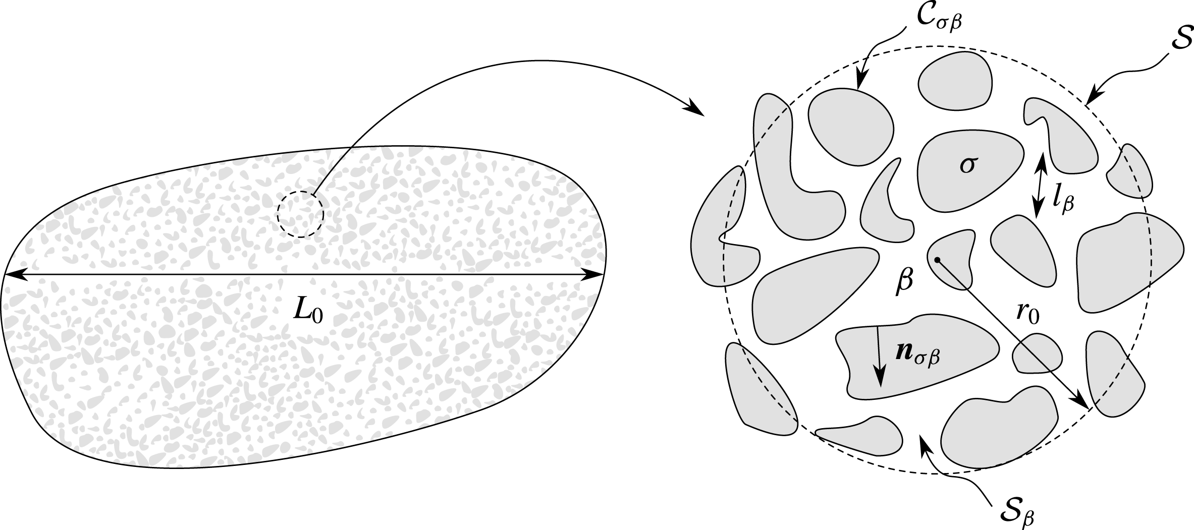
Figure 2. Macroscopic region and averaging surface of the fracture including the fluid phase
 $\unicode[STIX]{x1D6FD}$
and contact zones
$\unicode[STIX]{x1D6FD}$
and contact zones
 $\unicode[STIX]{x1D70E}$
.
$\unicode[STIX]{x1D70E}$
.
3.1 Volume averaging and unclosed macroscopic model
The derivation of the macroscale slip flow model from (2.28) starts with the application of the superficial average operator to the continuity equation (2.28a ). Making use of the spatial averaging theorem, this leads to
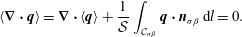 $$\begin{eqnarray}\langle \unicode[STIX]{x1D735}\boldsymbol{\cdot }\boldsymbol{q}\rangle =\unicode[STIX]{x1D735}\boldsymbol{\cdot }\langle \boldsymbol{q}\rangle +{\displaystyle \frac{1}{{\mathcal{S}}}}\int _{{\mathcal{C}}_{\unicode[STIX]{x1D70E}\unicode[STIX]{x1D6FD}}}^{}\boldsymbol{q}\boldsymbol{\cdot }\boldsymbol{n}_{\boldsymbol{\unicode[STIX]{x1D70E}}\boldsymbol{\unicode[STIX]{x1D6FD}}}\,\text{d}l=0.\end{eqnarray}$$
When the boundary condition in (2.28d ) is taken into account, this readily gives
 $$\begin{eqnarray}\unicode[STIX]{x1D735}\boldsymbol{\cdot }\langle \boldsymbol{q}\rangle =0.\end{eqnarray}$$
Attention can now be focused on the average of (2.28b
), and careful attention must first be paid to the mean free path present in this expression of the mass flow rate. If molecular collisions are assumed to be represented by pair collisions between hard spheres,
 $\unicode[STIX]{x1D706}$
depends on the inverse of the gas density according to (Loeb Reference Loeb2004)
$\unicode[STIX]{x1D706}$
depends on the inverse of the gas density according to (Loeb Reference Loeb2004)
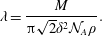 $$\begin{eqnarray}\unicode[STIX]{x1D706}={\displaystyle \frac{M}{\unicode[STIX]{x03C0}\sqrt{2}\unicode[STIX]{x1D6FF}^{2}{\mathcal{N}}_{A}\unicode[STIX]{x1D70C}}}.\end{eqnarray}$$
In this expression,
 $M$
is the molar mass of the gas,
$M$
is the molar mass of the gas,
 ${\mathcal{N}}_{A}$
is the Avogadro number and
${\mathcal{N}}_{A}$
is the Avogadro number and
 $\unicode[STIX]{x1D6FF}$
denotes the effective collision diameter of gas molecules. In many situations of practical interest, the flow can be considered as slightly compressible at the scale of the RES, which means that variations of the fluid-phase density remain small compared with the average density at the scale
$\unicode[STIX]{x1D6FF}$
denotes the effective collision diameter of gas molecules. In many situations of practical interest, the flow can be considered as slightly compressible at the scale of the RES, which means that variations of the fluid-phase density remain small compared with the average density at the scale
 $r_{0}$
, even though
$r_{0}$
, even though
 $\unicode[STIX]{x1D70C}$
can exhibit significant variations at the macroscopic scale
$\unicode[STIX]{x1D70C}$
can exhibit significant variations at the macroscopic scale
 $L_{0}$
. This assumption is adopted in the remainder of this work through the constraint (Quintard & Whitaker Reference Quintard and Whitaker1996; Lasseux et al.
Reference Lasseux, Valdes Parada, Ochoa Tapia and Goyeau2014)
$L_{0}$
. This assumption is adopted in the remainder of this work through the constraint (Quintard & Whitaker Reference Quintard and Whitaker1996; Lasseux et al.
Reference Lasseux, Valdes Parada, Ochoa Tapia and Goyeau2014)
 $$\begin{eqnarray}\widetilde{\unicode[STIX]{x1D70C}}\ll \langle \unicode[STIX]{x1D70C}\rangle ^{\unicode[STIX]{x1D6FD}}.\end{eqnarray}$$
With this hypothesis and from the decomposition of
 $\unicode[STIX]{x1D70C}$
(see (3.5)),
$\unicode[STIX]{x1D70C}$
(see (3.5)),
 $\unicode[STIX]{x1D706}$
can be considered as a constant at the scale
$\unicode[STIX]{x1D706}$
can be considered as a constant at the scale
 $r_{0}$
, so that its average, denoted
$r_{0}$
, so that its average, denoted
 $\bar{\unicode[STIX]{x1D706}}$
, is simplified to the following expression (Lasseux et al.
Reference Lasseux, Valdes Parada, Ochoa Tapia and Goyeau2014, Reference Lasseux, Valdés Parada and Porter2016):
$\bar{\unicode[STIX]{x1D706}}$
, is simplified to the following expression (Lasseux et al.
Reference Lasseux, Valdes Parada, Ochoa Tapia and Goyeau2014, Reference Lasseux, Valdés Parada and Porter2016):
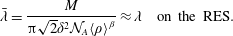 $$\begin{eqnarray}\bar{\unicode[STIX]{x1D706}}={\displaystyle \frac{M}{\unicode[STIX]{x03C0}\sqrt{2}\unicode[STIX]{x1D6FF}^{2}{\mathcal{N}}_{A}\langle \unicode[STIX]{x1D70C}\rangle ^{\unicode[STIX]{x1D6FD}}}}\approx \unicode[STIX]{x1D706}\quad \text{on the RES}.\end{eqnarray}$$
The averaging process can now be continued, and when the superficial average of (2.28b ) is formed while taking into account the slightly compressible assumption, one obtains
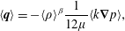 $$\begin{eqnarray}\langle \boldsymbol{q}\rangle =-\langle \unicode[STIX]{x1D70C}\rangle ^{\unicode[STIX]{x1D6FD}}{\displaystyle \frac{1}{12\unicode[STIX]{x1D707}}}\langle k\unicode[STIX]{x1D735}p\rangle ,\end{eqnarray}$$
where
 $k$
is given by
$k$
is given by
 $$\begin{eqnarray}k=h^{3}+\unicode[STIX]{x1D6FC}h^{2}\end{eqnarray}$$
and
 $$\begin{eqnarray}\unicode[STIX]{x1D6FC}=6\unicode[STIX]{x1D709}\bar{\unicode[STIX]{x1D706}}.\end{eqnarray}$$
Equation (3.13) represents the unclosed form of the average mass flow rate per unit width as it involves the pressure gradient at the roughness scale
 $l_{\unicode[STIX]{x1D6FD}}$
.
$l_{\unicode[STIX]{x1D6FD}}$
.
Before switching to the closure, the gas state law has to be expressed in its macroscopic form. Due to the slightly compressible hypothesis, it can be easily shown that the average of (2.1c ) yields (see section III.C in Lasseux et al. (Reference Lasseux, Valdes Parada, Ochoa Tapia and Goyeau2014))
 $$\begin{eqnarray}\langle \unicode[STIX]{x1D70C}\rangle ^{\unicode[STIX]{x1D6FD}}=\unicode[STIX]{x1D711}(\langle p\rangle ^{\unicode[STIX]{x1D6FD}}).\end{eqnarray}$$
3.2 Closure problem
To progress towards a closed form of the macroscopic flow model, equations (3.13) and (3.9) may be combined, and when the result is subtracted from the analogue combination of (2.28b ) and (2.28a ) together with the slightly compressible assumption, one obtains
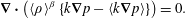 $$\begin{eqnarray}\unicode[STIX]{x1D735}\boldsymbol{\cdot }\left(\langle \unicode[STIX]{x1D70C}\rangle ^{\unicode[STIX]{x1D6FD}}\left\{k\unicode[STIX]{x1D735}p-\langle k\unicode[STIX]{x1D735}p\rangle \right\}\right)=0.\end{eqnarray}$$
When the pressure decomposition as defined by (3.5) is further employed, this last expression takes the form
 $$\begin{eqnarray}\unicode[STIX]{x1D735}\boldsymbol{\cdot }\left(\langle \unicode[STIX]{x1D70C}\rangle ^{\unicode[STIX]{x1D6FD}}\left\{k^{\ast }\unicode[STIX]{x1D735}\langle p\rangle ^{\unicode[STIX]{x1D6FD}}+k\unicode[STIX]{x1D735}\widetilde{p}-\langle k\unicode[STIX]{x1D735}\widetilde{p}\rangle \right\}\right)=0,\end{eqnarray}$$
with
 $$\begin{eqnarray}k^{\ast }=k-\langle k\rangle .\end{eqnarray}$$
In (3.18),
 $\unicode[STIX]{x1D735}\langle p\rangle ^{\unicode[STIX]{x1D6FD}}$
was treated as a constant within the averaging surface and was thus taken out of the averaging operator. This is justified by the constraint
$\unicode[STIX]{x1D735}\langle p\rangle ^{\unicode[STIX]{x1D6FD}}$
was treated as a constant within the averaging surface and was thus taken out of the averaging operator. This is justified by the constraint
 $r_{0}\ll L_{p1}$
, where
$r_{0}\ll L_{p1}$
, where
 $L_{p1}$
represents the characteristic length scale over which the first derivative of the average pressure exhibits significant variations (see Whitaker (Reference Whitaker1999)). Since
$L_{p1}$
represents the characteristic length scale over which the first derivative of the average pressure exhibits significant variations (see Whitaker (Reference Whitaker1999)). Since
 $L_{p1}$
is expected to be of the same order as
$L_{p1}$
is expected to be of the same order as
 $L_{0}$
, this constraint is equivalent to (3.4).
$L_{0}$
, this constraint is equivalent to (3.4).
Equation (3.18) can now be simplified by performing an order of magnitude analysis. Directing our attention to the boundary condition in (2.28d ), which can be written as
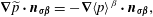 $$\begin{eqnarray}\unicode[STIX]{x1D735}\widetilde{p}\boldsymbol{\cdot }\boldsymbol{n}_{\unicode[STIX]{x1D748}\unicode[STIX]{x1D737}}=-\unicode[STIX]{x1D735}\langle p\rangle ^{\unicode[STIX]{x1D6FD}}\boldsymbol{\cdot }\boldsymbol{n}_{\unicode[STIX]{x1D748}\unicode[STIX]{x1D737}},\end{eqnarray}$$
the following order of magnitude estimate for
 $\widetilde{p}$
is obtained:
$\widetilde{p}$
is obtained:
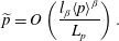 $$\begin{eqnarray}\widetilde{p}=O\left({\displaystyle \frac{l_{\unicode[STIX]{x1D6FD}}\langle p\rangle ^{\unicode[STIX]{x1D6FD}}}{L_{p}}}\right).\end{eqnarray}$$
In (3.21), the characteristic length scales of variation of
 $\widetilde{p}$
and
$\widetilde{p}$
and
 $\langle p\rangle ^{\unicode[STIX]{x1D6FD}}$
were respectively taken as
$\langle p\rangle ^{\unicode[STIX]{x1D6FD}}$
were respectively taken as
 $l_{\unicode[STIX]{x1D6FD}}$
and
$l_{\unicode[STIX]{x1D6FD}}$
and
 $L_{p}$
, with the idea that
$L_{p}$
, with the idea that
 $L_{p}\sim L_{0}$
. On this basis, the orders of magnitude of the last two terms on the left-hand side of (3.18) can be expressed as
$L_{p}\sim L_{0}$
. On this basis, the orders of magnitude of the last two terms on the left-hand side of (3.18) can be expressed as
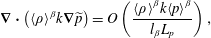 $$\begin{eqnarray}\displaystyle & \displaystyle \unicode[STIX]{x1D735}\boldsymbol{\cdot }\left(\langle \unicode[STIX]{x1D70C}\rangle ^{\unicode[STIX]{x1D6FD}}k\unicode[STIX]{x1D735}\widetilde{p}\right)=O\left({\displaystyle \frac{\langle \unicode[STIX]{x1D70C}\rangle ^{\unicode[STIX]{x1D6FD}}k\langle p\rangle ^{\unicode[STIX]{x1D6FD}}}{l_{\unicode[STIX]{x1D6FD}}L_{p}}}\right), & \displaystyle\end{eqnarray}$$
 $$\begin{eqnarray}\displaystyle & \displaystyle \unicode[STIX]{x1D735}\boldsymbol{\cdot }\left(\langle \unicode[STIX]{x1D70C}\rangle ^{\unicode[STIX]{x1D6FD}}\langle k\unicode[STIX]{x1D735}\widetilde{p}\rangle \right)=O\left({\displaystyle \frac{\langle \unicode[STIX]{x1D70C}\rangle ^{\unicode[STIX]{x1D6FD}}k\langle p\rangle ^{\unicode[STIX]{x1D6FD}}}{L_{0}L_{p}}}\right). & \displaystyle\end{eqnarray}$$
Due to the scale hierarchy (see relation (3.4)), the last term on the left-hand side of (3.18) can be neglected, and this yields
 $$\begin{eqnarray}\langle \unicode[STIX]{x1D70C}\rangle ^{\unicode[STIX]{x1D6FD}}\unicode[STIX]{x1D735}k^{\ast }\boldsymbol{\cdot }\unicode[STIX]{x1D735}\langle p\rangle ^{\unicode[STIX]{x1D6FD}}+k^{\ast }\unicode[STIX]{x1D735}\boldsymbol{\cdot }\left(\langle \unicode[STIX]{x1D70C}\rangle ^{\unicode[STIX]{x1D6FD}}\unicode[STIX]{x1D735}\langle p\rangle ^{\unicode[STIX]{x1D6FD}}\right)+\langle \unicode[STIX]{x1D70C}\rangle ^{\unicode[STIX]{x1D6FD}}\unicode[STIX]{x1D735}\boldsymbol{\cdot }\left(k\unicode[STIX]{x1D735}\widetilde{p}\right)+k\unicode[STIX]{x1D735}\widetilde{p}\boldsymbol{\cdot }\unicode[STIX]{x1D735}\langle \unicode[STIX]{x1D70C}\rangle ^{\unicode[STIX]{x1D6FD}}=0.\end{eqnarray}$$
Again, an order of magnitude analysis can be performed to estimate each of the terms of this last expression, and this gives
 $$\begin{eqnarray}\displaystyle & \displaystyle \langle \unicode[STIX]{x1D70C}\rangle ^{\unicode[STIX]{x1D6FD}}\unicode[STIX]{x1D735}k^{\ast }\boldsymbol{\cdot }\unicode[STIX]{x1D735}\langle p\rangle ^{\unicode[STIX]{x1D6FD}}=O\left({\displaystyle \frac{\langle \unicode[STIX]{x1D70C}\rangle ^{\unicode[STIX]{x1D6FD}}k^{\ast }\langle p\rangle ^{\unicode[STIX]{x1D6FD}}}{L_{p}l_{\unicode[STIX]{x1D6FD}}}}\right), & \displaystyle\end{eqnarray}$$
 $$\begin{eqnarray}\displaystyle & \displaystyle k^{\ast }\unicode[STIX]{x1D735}\boldsymbol{\cdot }\left(\langle \unicode[STIX]{x1D70C}\rangle ^{\unicode[STIX]{x1D6FD}}\unicode[STIX]{x1D735}\langle p\rangle ^{\unicode[STIX]{x1D6FD}}\right)=O\left({\displaystyle \frac{\langle \unicode[STIX]{x1D70C}\rangle ^{\unicode[STIX]{x1D6FD}}k^{\ast }\langle p\rangle ^{\unicode[STIX]{x1D6FD}}}{L_{p}L_{0}}}\right), & \displaystyle\end{eqnarray}$$
 $$\begin{eqnarray}\displaystyle & \displaystyle \langle \unicode[STIX]{x1D70C}\rangle ^{\unicode[STIX]{x1D6FD}}\unicode[STIX]{x1D735}\boldsymbol{\cdot }\left(k\unicode[STIX]{x1D735}\widetilde{p}\right)=O\left({\displaystyle \frac{\langle \unicode[STIX]{x1D70C}\rangle ^{\unicode[STIX]{x1D6FD}}k\widetilde{p}}{l_{\unicode[STIX]{x1D6FD}}^{2}}}\right), & \displaystyle\end{eqnarray}$$
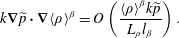 $$\begin{eqnarray}\displaystyle & \displaystyle k\unicode[STIX]{x1D735}\widetilde{p}\boldsymbol{\cdot }\unicode[STIX]{x1D735}\langle \unicode[STIX]{x1D70C}\rangle ^{\unicode[STIX]{x1D6FD}}=O\left({\displaystyle \frac{\langle \unicode[STIX]{x1D70C}\rangle ^{\unicode[STIX]{x1D6FD}}k\widetilde{p}}{L_{\unicode[STIX]{x1D70C}}l_{\unicode[STIX]{x1D6FD}}}}\right). & \displaystyle\end{eqnarray}$$
For the last term,
 $L_{\unicode[STIX]{x1D70C}}$
was used to designate the characteristic length of variation of
$L_{\unicode[STIX]{x1D70C}}$
was used to designate the characteristic length of variation of
 $\langle \unicode[STIX]{x1D70C}\rangle ^{\unicode[STIX]{x1D6FD}}$
, with again
$\langle \unicode[STIX]{x1D70C}\rangle ^{\unicode[STIX]{x1D6FD}}$
, with again
 $L_{\unicode[STIX]{x1D70C}}\sim L_{0}$
. The same argument of scale hierarchy (i.e.
$L_{\unicode[STIX]{x1D70C}}\sim L_{0}$
. The same argument of scale hierarchy (i.e.
 $l_{\unicode[STIX]{x1D6FD}}\ll L_{0}$
) can be invoked to conclude that the second and fourth terms on the left-hand side of expression (3.24) are negligible. Consequently, equation (3.17) finally takes the following simplified form:
$l_{\unicode[STIX]{x1D6FD}}\ll L_{0}$
) can be invoked to conclude that the second and fourth terms on the left-hand side of expression (3.24) are negligible. Consequently, equation (3.17) finally takes the following simplified form:
 $$\begin{eqnarray}\unicode[STIX]{x1D735}k^{\ast }\boldsymbol{\cdot }\unicode[STIX]{x1D735}\langle p\rangle ^{\unicode[STIX]{x1D6FD}}+\unicode[STIX]{x1D735}\boldsymbol{\cdot }\left(k\unicode[STIX]{x1D735}\widetilde{p}\right)=0.\end{eqnarray}$$
Equation (3.29) together with the associated boundary condition given by (3.20) forms the closure problem, although additional external boundary conditions are still required. Nevertheless, it should be clear that the goal is not to solve the closure problem over the entire structure. Instead, it can be solved on a portion that contains all of the structural information (i.e. an RES), allowing a pseudoperiodic representation of the whole fracture while applying a periodic boundary condition on the pressure deviation
 $\widetilde{p}$
on the RES. Such a condition can be written as
$\widetilde{p}$
on the RES. Such a condition can be written as
 $$\begin{eqnarray}\widetilde{p}(\boldsymbol{x}+\unicode[STIX]{x1D72B}_{\boldsymbol{i}})=\widetilde{p}(\boldsymbol{x}),\quad i=x,y,\end{eqnarray}$$
where
 $\boldsymbol{x}$
is a position vector locating any point in the averaging surface and
$\boldsymbol{x}$
is a position vector locating any point in the averaging surface and
 $\unicode[STIX]{x1D72B}_{\boldsymbol{i}}$
represents the two lattice vectors required to describe the spatially periodic rough structure. The local closure problem for
$\unicode[STIX]{x1D72B}_{\boldsymbol{i}}$
represents the two lattice vectors required to describe the spatially periodic rough structure. The local closure problem for
 $\widetilde{p}$
can hence be stated as
$\widetilde{p}$
can hence be stated as
 $$\begin{eqnarray}\displaystyle & \displaystyle \unicode[STIX]{x1D735}\boldsymbol{\cdot }\left(k\unicode[STIX]{x1D735}\widetilde{p}\right)=-\unicode[STIX]{x1D735}k^{\ast }\boldsymbol{\cdot }\unicode[STIX]{x1D735}\langle p\rangle ^{\unicode[STIX]{x1D6FD}}\quad \text{in }{\mathcal{S}}_{\unicode[STIX]{x1D6FD}}, & \displaystyle\end{eqnarray}$$
 $$\begin{eqnarray}\displaystyle & \displaystyle \unicode[STIX]{x1D735}\widetilde{p}\boldsymbol{\cdot }\boldsymbol{n}_{\unicode[STIX]{x1D748}\unicode[STIX]{x1D737}}=-\unicode[STIX]{x1D735}\langle p\rangle ^{\unicode[STIX]{x1D6FD}}\boldsymbol{\cdot }\boldsymbol{n}_{\unicode[STIX]{x1D748}\unicode[STIX]{x1D737}}\quad \text{at }{\mathcal{C}}_{\unicode[STIX]{x1D70E}\unicode[STIX]{x1D6FD}}, & \displaystyle\end{eqnarray}$$
 $$\begin{eqnarray}\displaystyle & \displaystyle \widetilde{p}(\boldsymbol{x}+\unicode[STIX]{x1D72B}_{\boldsymbol{i}})=\widetilde{p}(\boldsymbol{x}),\quad i=x,y. & \displaystyle\end{eqnarray}$$
Since this problem on
 $\widetilde{p}$
is linear, the solution can be sought as a linear combination of the sources that make it non-homogeneous. Here,
$\widetilde{p}$
is linear, the solution can be sought as a linear combination of the sources that make it non-homogeneous. Here,
 $\unicode[STIX]{x1D735}\langle p\rangle ^{\unicode[STIX]{x1D6FD}}$
acts as the unique source term and the pressure deviation field can hence be determined with the following representation:
$\unicode[STIX]{x1D735}\langle p\rangle ^{\unicode[STIX]{x1D6FD}}$
acts as the unique source term and the pressure deviation field can hence be determined with the following representation:
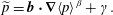 $$\begin{eqnarray}\widetilde{p}=\boldsymbol{b}\boldsymbol{\cdot }\unicode[STIX]{x1D735}\langle p\rangle ^{\unicode[STIX]{x1D6FD}}+\unicode[STIX]{x1D6FE}.\end{eqnarray}$$
Here,
 $\boldsymbol{b}$
is the closure vector while
$\boldsymbol{b}$
is the closure vector while
 $\unicode[STIX]{x1D6FE}$
is an arbitrary function. On substituting the representation (3.32) into (3.31) and keeping in mind that
$\unicode[STIX]{x1D6FE}$
is an arbitrary function. On substituting the representation (3.32) into (3.31) and keeping in mind that
 $\unicode[STIX]{x1D6FE}$
is arbitrary,
$\unicode[STIX]{x1D6FE}$
is arbitrary,
 $\boldsymbol{b}$
can be chosen to obey the following boundary-value problem:
$\boldsymbol{b}$
can be chosen to obey the following boundary-value problem:
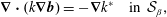 $$\begin{eqnarray}\displaystyle & \displaystyle \unicode[STIX]{x1D735}\boldsymbol{\cdot }\left(k\unicode[STIX]{x1D735}\boldsymbol{b}\right)=-\unicode[STIX]{x1D735}k^{\ast }\quad \text{in }{\mathcal{S}}_{\unicode[STIX]{x1D6FD}}, & \displaystyle\end{eqnarray}$$
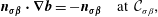 $$\begin{eqnarray}\displaystyle & \displaystyle \boldsymbol{n}_{\unicode[STIX]{x1D748}\unicode[STIX]{x1D737}}\boldsymbol{\cdot }\unicode[STIX]{x1D735}\boldsymbol{b}=-\boldsymbol{n}_{\unicode[STIX]{x1D748}\unicode[STIX]{x1D737}}\quad \text{at }{\mathcal{C}}_{\unicode[STIX]{x1D70E}\unicode[STIX]{x1D6FD}}, & \displaystyle\end{eqnarray}$$
 $$\begin{eqnarray}\displaystyle & \displaystyle \boldsymbol{b}(\boldsymbol{x}+\unicode[STIX]{x1D72B}_{\boldsymbol{i}})=\boldsymbol{b}(\boldsymbol{x}),\quad i=x,y. & \displaystyle\end{eqnarray}$$
With such a choice for the closure problem on
 $\boldsymbol{b}$
, it can be shown that
$\boldsymbol{b}$
, it can be shown that
 $\unicode[STIX]{x1D6FE}$
is a constant, which thus has no impact on the final macroscopic model. The proof is provided in appendix A. The closure procedure can now be completed by expressing the macroscopic model as detailed in the next section.
$\unicode[STIX]{x1D6FE}$
is a constant, which thus has no impact on the final macroscopic model. The proof is provided in appendix A. The closure procedure can now be completed by expressing the macroscopic model as detailed in the next section.
3.3 Macroscopic flow model
The pressure decomposition together with the deviation representation (3.32) can now be introduced in (3.13) to obtain the closed macroscopic expression of the mass flow rate per unit width of the fracture as
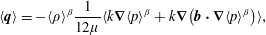 $$\begin{eqnarray}\langle \boldsymbol{q}\rangle =-\langle \unicode[STIX]{x1D70C}\rangle ^{\unicode[STIX]{x1D6FD}}{\displaystyle \frac{1}{12\unicode[STIX]{x1D707}}}\langle k\unicode[STIX]{x1D735}\langle p\rangle ^{\unicode[STIX]{x1D6FD}}+k\unicode[STIX]{x1D735}\left(\boldsymbol{b}\boldsymbol{\cdot }\unicode[STIX]{x1D735}\langle p\rangle ^{\unicode[STIX]{x1D6FD}}\right)\rangle ,\end{eqnarray}$$
or, since
 $\unicode[STIX]{x1D735}\langle p\rangle ^{\unicode[STIX]{x1D6FD}}$
can be treated as a constant at the scale of the RES,
$\unicode[STIX]{x1D735}\langle p\rangle ^{\unicode[STIX]{x1D6FD}}$
can be treated as a constant at the scale of the RES,
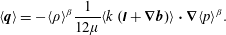 $$\begin{eqnarray}\langle \boldsymbol{q}\rangle =-\langle \unicode[STIX]{x1D70C}\rangle ^{\unicode[STIX]{x1D6FD}}{\displaystyle \frac{1}{12\unicode[STIX]{x1D707}}}\langle k\left(\unicode[STIX]{x1D644}+\unicode[STIX]{x1D735}\boldsymbol{b}\right)\rangle \boldsymbol{\cdot }\unicode[STIX]{x1D735}\langle p\rangle ^{\unicode[STIX]{x1D6FD}}.\end{eqnarray}$$
As a summary, the macroscopic Reynolds model for slightly compressible slip flow in a fracture is given by
 $$\begin{eqnarray}\displaystyle & \displaystyle \unicode[STIX]{x1D735}\boldsymbol{\cdot }\langle \boldsymbol{q}\rangle =0, & \displaystyle\end{eqnarray}$$
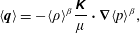 $$\begin{eqnarray}\displaystyle & \displaystyle \langle \boldsymbol{q}\rangle =-\langle \unicode[STIX]{x1D70C}\rangle ^{\unicode[STIX]{x1D6FD}}{\displaystyle \frac{\unicode[STIX]{x1D646}}{\unicode[STIX]{x1D707}}}\boldsymbol{\cdot }\unicode[STIX]{x1D735}\langle p\rangle ^{\unicode[STIX]{x1D6FD}}, & \displaystyle\end{eqnarray}$$
 $$\begin{eqnarray}\displaystyle & \displaystyle \langle \unicode[STIX]{x1D70C}\rangle ^{\unicode[STIX]{x1D6FD}}=\unicode[STIX]{x1D711}(\langle p\rangle ^{\unicode[STIX]{x1D6FD}}), & \displaystyle\end{eqnarray}$$
 $\unicode[STIX]{x1D646}$
is the macroscopic transmissivity tensor, defined as
$\unicode[STIX]{x1D646}$
is the macroscopic transmissivity tensor, defined as 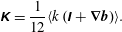 $$\begin{eqnarray}\unicode[STIX]{x1D646}={\displaystyle \frac{1}{12}}\langle k\left(\unicode[STIX]{x1D644}+\unicode[STIX]{x1D735}\boldsymbol{b}\right)\rangle .\end{eqnarray}$$
The macroscopic transmissivity tensor is entirely determined from the solution of the closure problem (3.33) on
 $\boldsymbol{b}$
. It should be noted that this problem defines
$\boldsymbol{b}$
. It should be noted that this problem defines
 $\boldsymbol{b}$
to within an additive constant, which has, however, no impact on
$\boldsymbol{b}$
to within an additive constant, which has, however, no impact on
 $\unicode[STIX]{x1D646}$
. Moreover, the closure problem is not intrinsic as it depends not only on the local aperture of the fracture but also on the average density
$\unicode[STIX]{x1D646}$
. Moreover, the closure problem is not intrinsic as it depends not only on the local aperture of the fracture but also on the average density
 $\langle \unicode[STIX]{x1D70C}\rangle ^{\unicode[STIX]{x1D6FD}}$
(or on the reference mean free path
$\langle \unicode[STIX]{x1D70C}\rangle ^{\unicode[STIX]{x1D6FD}}$
(or on the reference mean free path
 $\bar{\unicode[STIX]{x1D706}}$
), which is implicitly present in
$\bar{\unicode[STIX]{x1D706}}$
), which is implicitly present in
 $k$
, featuring a non-intrinsic tensor
$k$
, featuring a non-intrinsic tensor
 $\unicode[STIX]{x1D646}$
. The transmissivity tensor can be shown to be symmetric regardless the aperture field structure (Lasseux & Valdes Parada Reference Lasseux and Valdes Parada2017).
$\unicode[STIX]{x1D646}$
. The transmissivity tensor can be shown to be symmetric regardless the aperture field structure (Lasseux & Valdes Parada Reference Lasseux and Valdes Parada2017).
3.4 Decomposition of the closure
As indicated in the previous section, the closure problem on
 $\boldsymbol{b}$
is not intrinsic and yields a transmissivity tensor
$\boldsymbol{b}$
is not intrinsic and yields a transmissivity tensor
 $\unicode[STIX]{x1D646}$
lumping together viscous and slip effects. In order to exhibit the particular role of the slip at the fracture walls, a further development of the closure problem is carried out.
$\unicode[STIX]{x1D646}$
lumping together viscous and slip effects. In order to exhibit the particular role of the slip at the fracture walls, a further development of the closure problem is carried out.
Let us first reformulate (3.33a
) by introducing the decomposition of
 $k$
given in the relationship (3.19), to obtain
$k$
given in the relationship (3.19), to obtain
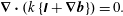 $$\begin{eqnarray}\unicode[STIX]{x1D735}\boldsymbol{\cdot }\left(k\left\{\unicode[STIX]{x1D644}+\unicode[STIX]{x1D735}\boldsymbol{b}\right\}\right)=0.\end{eqnarray}$$
To arrive at this result, we have used the fact that
 $k^{\ast }$
and
$k^{\ast }$
and
 $\langle k\rangle$
are of the same order of magnitude along with the length-scale contrast
$\langle k\rangle$
are of the same order of magnitude along with the length-scale contrast
 $l_{\unicode[STIX]{x1D6FD}}\ll L_{0}$
, so that
$l_{\unicode[STIX]{x1D6FD}}\ll L_{0}$
, so that
 $\unicode[STIX]{x1D735}\langle k\rangle \ll \unicode[STIX]{x1D735}k^{\ast }$
. The closure problem is now rewritten in a dimensionless form as
$\unicode[STIX]{x1D735}\langle k\rangle \ll \unicode[STIX]{x1D735}k^{\ast }$
. The closure problem is now rewritten in a dimensionless form as
 $$\begin{eqnarray}\displaystyle & \displaystyle \text{}\underline{\boldsymbol{\unicode[STIX]{x1D6FB}}}\boldsymbol{\cdot }\left(\text{}\underline{k}\left\{\unicode[STIX]{x1D644}+\text{}\underline{\unicode[STIX]{x1D735}}\text{}\underline{\boldsymbol{b}}\right\}\right)=0\quad \text{in }{\mathcal{S}}_{\unicode[STIX]{x1D6FD}}, & \displaystyle\end{eqnarray}$$
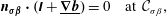 $$\begin{eqnarray}\displaystyle & \displaystyle \boldsymbol{n}_{\unicode[STIX]{x1D748}\unicode[STIX]{x1D737}}\boldsymbol{\cdot }\left(\unicode[STIX]{x1D644}+\text{}\underline{\unicode[STIX]{x1D735}}\text{}\underline{\boldsymbol{b}}\right)=0\quad \text{at }{\mathcal{C}}_{\unicode[STIX]{x1D70E}\unicode[STIX]{x1D6FD}}, & \displaystyle\end{eqnarray}$$
 $$\begin{eqnarray}\displaystyle & \displaystyle \text{}\underline{\boldsymbol{b}}(\text{}\underline{\boldsymbol{x}}+\text{}\underline{\unicode[STIX]{x1D72B}_{\boldsymbol{i}}})=\text{}\underline{\boldsymbol{b}}(\text{}\underline{\boldsymbol{x}}),\quad i=x,y, & \displaystyle\end{eqnarray}$$
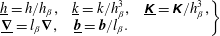 $$\begin{eqnarray}\displaystyle \left.\begin{array}{@{}ccc@{}}\text{}\underline{h}=h/h_{\unicode[STIX]{x1D6FD}}, & \text{}\underline{k}=k/h_{\unicode[STIX]{x1D6FD}}^{3}, & \text{}\underline{\unicode[STIX]{x1D646}}=\unicode[STIX]{x1D646}/h_{\unicode[STIX]{x1D6FD}}^{3},\\ \text{}\underline{\unicode[STIX]{x1D735}}=l_{\unicode[STIX]{x1D6FD}}\unicode[STIX]{x1D735}, & \text{}\underline{\boldsymbol{b}}=\boldsymbol{b}/l_{\unicode[STIX]{x1D6FD}}.\end{array}\right\} & & \displaystyle\end{eqnarray}$$
As before,
 $h_{\unicode[STIX]{x1D6FD}}$
is the characteristic aperture of the fracture over the RES and
$h_{\unicode[STIX]{x1D6FD}}$
is the characteristic aperture of the fracture over the RES and
 $l_{\unicode[STIX]{x1D6FD}}$
is the characteristic roughness length scale. In addition, the Knudsen number
$l_{\unicode[STIX]{x1D6FD}}$
is the characteristic roughness length scale. In addition, the Knudsen number
 $\overline{Kn}$
associated with the reference mean free path
$\overline{Kn}$
associated with the reference mean free path
 $\bar{\unicode[STIX]{x1D706}}$
is defined as
$\bar{\unicode[STIX]{x1D706}}$
is defined as
 $$\begin{eqnarray}\overline{Kn}=\bar{\unicode[STIX]{x1D706}}/h_{\unicode[STIX]{x1D6FD}},\end{eqnarray}$$
on which
 $\text{}\underline{k}$
explicitly depends according to
$\text{}\underline{k}$
explicitly depends according to
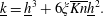 $$\begin{eqnarray}\text{}\underline{k}=\text{}\underline{h}^{3}+6\unicode[STIX]{x1D709}\overline{Kn}\text{}\underline{h}^{2}.\end{eqnarray}$$
The macroscopic dimensionless transmissivity tensor has the following expression:
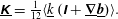 $$\begin{eqnarray}\text{}\underline{\unicode[STIX]{x1D646}}={\textstyle \frac{1}{12}}\langle \text{}\underline{k}\left(\unicode[STIX]{x1D644}+\text{}\underline{\unicode[STIX]{x1D735}}\text{}\underline{\boldsymbol{b}}\right)\rangle .\end{eqnarray}$$
Since the value of
 $\unicode[STIX]{x1D709}\overline{Kn}$
is constrained to remain smaller than unity in the slip regime (Karniadakis et al.
Reference Karniadakis, Beskok and Aluru2005), the dimensionless closure variable
$\unicode[STIX]{x1D709}\overline{Kn}$
is constrained to remain smaller than unity in the slip regime (Karniadakis et al.
Reference Karniadakis, Beskok and Aluru2005), the dimensionless closure variable
 $\text{}\underline{\boldsymbol{b}}$
may be expanded as a power series of this parameter under the form
$\text{}\underline{\boldsymbol{b}}$
may be expanded as a power series of this parameter under the form
 $$\begin{eqnarray}\text{}\underline{\boldsymbol{b}}=\text{}\underline{\boldsymbol{b}_{\mathbf{0}}}+6\unicode[STIX]{x1D709}\overline{Kn}\text{}\underline{\boldsymbol{b}_{\mathbf{1}}}+\left(6\unicode[STIX]{x1D709}\overline{Kn}\right)^{2}\text{}\underline{\boldsymbol{b}_{\boldsymbol{ 2}}}+\cdots \,,\end{eqnarray}$$
where each dimensionless closure variable
 $\text{}\underline{\boldsymbol{b}_{\boldsymbol{i}}}$
at the
$\text{}\underline{\boldsymbol{b}_{\boldsymbol{i}}}$
at the
 $i$
th order is defined as
$i$
th order is defined as
 $$\begin{eqnarray}\text{}\underline{\boldsymbol{b}_{\boldsymbol{i}}}={\displaystyle \frac{h_{\unicode[STIX]{x1D6FD}}^{i}}{l_{\unicode[STIX]{x1D6FD}}}}\boldsymbol{b}_{\boldsymbol{i}}.\end{eqnarray}$$
When the expansion in (3.44) along with the expression in (3.42) is introduced back into (3.39), the original problem can be split into two intrinsic but coupled closure subproblems at successive orders in
 $\unicode[STIX]{x1D709}\overline{Kn}$
. Returning to the dimensional form and restricting our analysis to the first order, one obtains the following.
$\unicode[STIX]{x1D709}\overline{Kn}$
. Returning to the dimensional form and restricting our analysis to the first order, one obtains the following.
Zeroth-order subproblem:
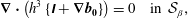 $$\begin{eqnarray}\displaystyle & \displaystyle \unicode[STIX]{x1D735}\boldsymbol{\cdot }\left(h^{3}\left\{\unicode[STIX]{x1D644}+\unicode[STIX]{x1D735}\boldsymbol{b}_{\mathbf{0}}\right\}\right)=0\quad \text{in }{\mathcal{S}}_{\unicode[STIX]{x1D6FD}}, & \displaystyle\end{eqnarray}$$
 $$\begin{eqnarray}\displaystyle & \displaystyle \boldsymbol{n}_{\unicode[STIX]{x1D748}\unicode[STIX]{x1D737}}\boldsymbol{\cdot }\left(\unicode[STIX]{x1D644}+\unicode[STIX]{x1D735}\boldsymbol{b}_{\mathbf{0}}\right)=0\quad \text{at }{\mathcal{C}}_{\unicode[STIX]{x1D70E}\unicode[STIX]{x1D6FD}}, & \displaystyle\end{eqnarray}$$
 $$\begin{eqnarray}\displaystyle & \displaystyle \boldsymbol{b}_{\mathbf{0}}(\boldsymbol{x}+\unicode[STIX]{x1D72B}_{\boldsymbol{i}})=\boldsymbol{b}_{\mathbf{0}}(\boldsymbol{x}),\quad i=x,y. & \displaystyle\end{eqnarray}$$
First-order subproblem:
 $$\begin{eqnarray}\displaystyle & \displaystyle \unicode[STIX]{x1D735}\boldsymbol{\cdot }\left(h^{3}\unicode[STIX]{x1D735}\boldsymbol{b}_{\mathbf{1}}\right)=-\unicode[STIX]{x1D735}\boldsymbol{\cdot }\left(h^{2}\left\{\unicode[STIX]{x1D644}+\unicode[STIX]{x1D735}\boldsymbol{b}_{\mathbf{0}}\right\}\right)\quad \text{in }{\mathcal{S}}_{\unicode[STIX]{x1D6FD}}, & \displaystyle\end{eqnarray}$$
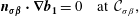 $$\begin{eqnarray}\displaystyle & \displaystyle \boldsymbol{n}_{\unicode[STIX]{x1D748}\unicode[STIX]{x1D737}}\boldsymbol{\cdot }\unicode[STIX]{x1D735}\boldsymbol{b}_{\mathbf{1}}=0\quad \text{at }{\mathcal{C}}_{\unicode[STIX]{x1D70E}\unicode[STIX]{x1D6FD}}, & \displaystyle\end{eqnarray}$$
 $$\begin{eqnarray}\displaystyle & \displaystyle \boldsymbol{b}_{\mathbf{1}}(\boldsymbol{x}+\unicode[STIX]{x1D72B}_{\boldsymbol{i}})=\boldsymbol{b}_{\mathbf{1}}(\boldsymbol{x}),\quad i=x,y. & \displaystyle\end{eqnarray}$$
Similarly, introduction of the relationships (3.42) and (3.44) into (3.43) allows one to write the dimensionless transmissivity tensor at the desired order in
 $\unicode[STIX]{x1D709}\overline{Kn}$
. Under a dimensional form and at the first order, this is written as
$\unicode[STIX]{x1D709}\overline{Kn}$
. Under a dimensional form and at the first order, this is written as
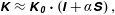 $$\begin{eqnarray}\unicode[STIX]{x1D646}\approx \unicode[STIX]{x1D646}_{\unicode[STIX]{x1D7EC}}\boldsymbol{\cdot }\left(\unicode[STIX]{x1D644}+\unicode[STIX]{x1D6FC}\unicode[STIX]{x1D64E}\right),\end{eqnarray}$$
where
 $\unicode[STIX]{x1D646}_{\unicode[STIX]{x1D7EC}}$
is the intrinsic transmissivity tensor, defined as
$\unicode[STIX]{x1D646}_{\unicode[STIX]{x1D7EC}}$
is the intrinsic transmissivity tensor, defined as
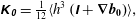 $$\begin{eqnarray}\unicode[STIX]{x1D646}_{\unicode[STIX]{x1D7EC}}={\textstyle \frac{1}{12}}\langle h^{3}\left(\unicode[STIX]{x1D644}+\unicode[STIX]{x1D735}\boldsymbol{b}_{\boldsymbol{ 0}}\right)\rangle ,\end{eqnarray}$$
and
 $\unicode[STIX]{x1D64E}$
is the intrinsic first order slip-correction tensor, the expression of which is given by
$\unicode[STIX]{x1D64E}$
is the intrinsic first order slip-correction tensor, the expression of which is given by
 $$\begin{eqnarray}\unicode[STIX]{x1D64E}={\textstyle \frac{1}{12}}\unicode[STIX]{x1D646}_{\unicode[STIX]{x1D7EC}}^{-1}\boldsymbol{\cdot }\langle h^{2}\left(\unicode[STIX]{x1D644}+\unicode[STIX]{x1D735}\boldsymbol{b}_{\boldsymbol{ 0}}\right)+h^{3}\unicode[STIX]{x1D735}\boldsymbol{b}_{\boldsymbol{ 1}}\rangle .\end{eqnarray}$$
The solution of the above two subproblems for
 $\boldsymbol{b}_{\mathbf{0}}$
and
$\boldsymbol{b}_{\mathbf{0}}$
and
 $\boldsymbol{b}_{\mathbf{1}}$
on the RES provides
$\boldsymbol{b}_{\mathbf{1}}$
on the RES provides
 $\unicode[STIX]{x1D646}_{\unicode[STIX]{x1D7EC}}$
and
$\unicode[STIX]{x1D646}_{\unicode[STIX]{x1D7EC}}$
and
 $\unicode[STIX]{x1D64E}$
, yielding a linear approximation of
$\unicode[STIX]{x1D64E}$
, yielding a linear approximation of
 $\unicode[STIX]{x1D646}$
in terms of the slip parameter
$\unicode[STIX]{x1D646}$
in terms of the slip parameter
 $\unicode[STIX]{x1D6FC}$
defined in (3.15). It should be noted that the zeroth-order subproblem exactly corresponds to that obtained on upscaling an incompressible Reynolds flow without slip at the solid–fluid boundary in a rough fracture (Prat et al.
Reference Prat, Plouraboué and Letalleur2002; Vallet et al.
Reference Vallet, Lasseux, Sainsot and Zahouani2009), yielding the intrinsic transmissivity tensor
$\unicode[STIX]{x1D6FC}$
defined in (3.15). It should be noted that the zeroth-order subproblem exactly corresponds to that obtained on upscaling an incompressible Reynolds flow without slip at the solid–fluid boundary in a rough fracture (Prat et al.
Reference Prat, Plouraboué and Letalleur2002; Vallet et al.
Reference Vallet, Lasseux, Sainsot and Zahouani2009), yielding the intrinsic transmissivity tensor
 $\unicode[STIX]{x1D646}_{\unicode[STIX]{x1D7EC}}$
, which is a signature of viscous effects only.
$\unicode[STIX]{x1D646}_{\unicode[STIX]{x1D7EC}}$
, which is a signature of viscous effects only.
The first-order approximation (3.48) of the macroscopic transmissivity tensor can be viewed as an analogue of the tensorial Klinkenberg apparent permeability (Klinkenberg Reference Klinkenberg1941) for gas slip flow in a two-dimensional porous medium. Indeed, the expression of the reference mean free path
 $\bar{\unicode[STIX]{x1D706}}$
in (3.12), which depends on the inverse of the average density
$\bar{\unicode[STIX]{x1D706}}$
in (3.12), which depends on the inverse of the average density
 $\langle \unicode[STIX]{x1D70C}\rangle ^{\unicode[STIX]{x1D6FD}}$
, takes the following form if the gas obeys an ideal gas law and the flow is quasi-isothermal (i.e.
$\langle \unicode[STIX]{x1D70C}\rangle ^{\unicode[STIX]{x1D6FD}}$
, takes the following form if the gas obeys an ideal gas law and the flow is quasi-isothermal (i.e.
 $\langle T\rangle ^{\unicode[STIX]{x1D6FD}}\gg \widetilde{T}$
) (Cercignani Reference Cercignani1988):
$\langle T\rangle ^{\unicode[STIX]{x1D6FD}}\gg \widetilde{T}$
) (Cercignani Reference Cercignani1988):
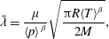 $$\begin{eqnarray}\bar{\unicode[STIX]{x1D706}}={\displaystyle \frac{\unicode[STIX]{x1D707}}{\langle p\rangle ^{\unicode[STIX]{x1D6FD}}}}\sqrt{{\displaystyle \frac{\unicode[STIX]{x03C0}R\langle T\rangle ^{\unicode[STIX]{x1D6FD}}}{2M}}},\end{eqnarray}$$
where
 $R$
is the ideal gas constant. Insertion of this last expression into (3.48) allows one to write the first-order approximation of
$R$
is the ideal gas constant. Insertion of this last expression into (3.48) allows one to write the first-order approximation of
 $\unicode[STIX]{x1D646}$
as a function of the inverse average pressure in a classical Klinkenberg-like formulation (Lasseux et al.
Reference Lasseux, Valdes Parada, Ochoa Tapia and Goyeau2014),
$\unicode[STIX]{x1D646}$
as a function of the inverse average pressure in a classical Klinkenberg-like formulation (Lasseux et al.
Reference Lasseux, Valdes Parada, Ochoa Tapia and Goyeau2014),
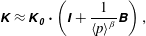 $$\begin{eqnarray}\unicode[STIX]{x1D646}\approx \unicode[STIX]{x1D646}_{\unicode[STIX]{x1D7EC}}\boldsymbol{\cdot }\left(\unicode[STIX]{x1D644}+{\displaystyle \frac{1}{\langle p\rangle ^{\unicode[STIX]{x1D6FD}}}}\unicode[STIX]{x1D63D}\right),\end{eqnarray}$$
 $\unicode[STIX]{x1D63D}$
being the two-dimensional tensorial Klinkenberg coefficient, defined as
$\unicode[STIX]{x1D63D}$
being the two-dimensional tensorial Klinkenberg coefficient, defined as
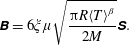 $$\begin{eqnarray}\unicode[STIX]{x1D63D}=6\unicode[STIX]{x1D709}\unicode[STIX]{x1D707}\sqrt{{\displaystyle \frac{\unicode[STIX]{x03C0}R\langle T\rangle ^{\unicode[STIX]{x1D6FD}}}{2M}}}\unicode[STIX]{x1D64E}.\end{eqnarray}$$
4 Numerical solutions to the closure problems
4.1 Validation on simple geometries
In this section, a numerical validation of the macroscopic flow model (3.36) is illustrated on simple aperture fields for which the complete macroscopic transmissivity tensor can be determined analytically from the local transmissivities in (2.28b
) and compared with that obtained from the solution of the closure problem given by (3.33). In the general case, the aperture field on the RES is varying in both the
 $x$
- and
$x$
- and
 $y$
-directions (i.e.
$y$
-directions (i.e.
 $h=h(x,y)$
). However, when
$h=h(x,y)$
). However, when
 $h$
depends on only one spatial coordinate (
$h$
depends on only one spatial coordinate (
 $x$
for instance), the aperture field can be assimilated to a set of conductivities arranged in a purely serial or parallel configuration when the pressure gradient is along
$x$
for instance), the aperture field can be assimilated to a set of conductivities arranged in a purely serial or parallel configuration when the pressure gradient is along
 $x$
or
$x$
or
 $y$
respectively. For a parallel configuration, the transmissivity,
$y$
respectively. For a parallel configuration, the transmissivity,
 $K_{p}$
, of the aperture field is given by the arithmetic mean of the local transmissivities (Zimmerman & Bodvarsson Reference Zimmerman and Bodvarsson1996),
$K_{p}$
, of the aperture field is given by the arithmetic mean of the local transmissivities (Zimmerman & Bodvarsson Reference Zimmerman and Bodvarsson1996),
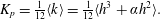 $$\begin{eqnarray}K_{p}={\textstyle \frac{1}{12}}\langle k\rangle ={\textstyle \frac{1}{12}}\langle h^{3}+\unicode[STIX]{x1D6FC}h^{2}\rangle .\end{eqnarray}$$
For a serial configuration, the transmissivity,
 $K_{s}$
, is the harmonic mean of the local transmissivities,
$K_{s}$
, is the harmonic mean of the local transmissivities,
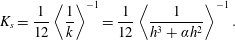 $$\begin{eqnarray}K_{s}={\displaystyle \frac{1}{12}}\left\langle {\displaystyle \frac{1}{k}}\right\rangle ^{-1}={\displaystyle \frac{1}{12}}\left\langle {\displaystyle \frac{1}{h^{3}+\unicode[STIX]{x1D6FC}h^{2}}}\right\rangle ^{-1}.\end{eqnarray}$$
In the following, two aperture fields varying with respect to the
 $x$
-direction only are analysed. They are defined for
$x$
-direction only are analysed. They are defined for
 $x\in \left[0,l_{x}\right]$
and have a mean value
$x\in \left[0,l_{x}\right]$
and have a mean value
 $h_{0}$
.
$h_{0}$
.
Sinusoidal aperture field
A sinusoidal aperture field is considered first, given by
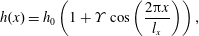 $$\begin{eqnarray}h(x)=h_{0}\left(1+\unicode[STIX]{x1D6F6}\cos \left(\frac{2\unicode[STIX]{x03C0}x}{l_{x}}\right)\right),\end{eqnarray}$$
where the amplitude,
 $\unicode[STIX]{x1D6F6}$
, is assumed to be smaller than unity (non-contact case) and
$\unicode[STIX]{x1D6F6}$
, is assumed to be smaller than unity (non-contact case) and
 $l_{x}$
corresponds to the spatial period. The determination of the parallel transmissivity with (4.1) is trivial in this case and gives
$l_{x}$
corresponds to the spatial period. The determination of the parallel transmissivity with (4.1) is trivial in this case and gives
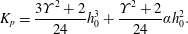 $$\begin{eqnarray}K_{p}={\displaystyle \frac{3\unicode[STIX]{x1D6F6}^{2}+2}{24}}h_{0}^{3}+{\displaystyle \frac{\unicode[STIX]{x1D6F6}^{2}+2}{24}}\unicode[STIX]{x1D6FC}h_{0}^{2}.\end{eqnarray}$$
The evaluation of the serial transmissivity, using (4.2), is a little more complex and requires the calculation of the following integral:
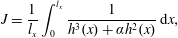 $$\begin{eqnarray}J={\displaystyle \frac{1}{l_{x}}}\int _{0}^{l_{x}}{\displaystyle \frac{1}{h^{3}(x)+\unicode[STIX]{x1D6FC}h^{2}(x)}}\,\text{d}x,\end{eqnarray}$$
while
 $K_{s}=J^{-1}/12$
. By performing a partial fraction decomposition of the integrand, (4.5) can be rewritten as
$K_{s}=J^{-1}/12$
. By performing a partial fraction decomposition of the integrand, (4.5) can be rewritten as
 $$\begin{eqnarray}J={\displaystyle \frac{1}{l_{x}}}\int _{0}^{l_{x}}{\displaystyle \frac{1}{\unicode[STIX]{x1D6FC}h^{2}(x)}}\,\text{d}x-{\displaystyle \frac{1}{l_{x}}}\int _{0}^{l_{x}}{\displaystyle \frac{1}{\unicode[STIX]{x1D6FC}^{2}h(x)}}\,\text{d}x+{\displaystyle \frac{1}{l_{x}}}\int _{0}^{l_{x}}{\displaystyle \frac{1}{\unicode[STIX]{x1D6FC}^{2}\left(h(x)+\unicode[STIX]{x1D6FC}\right)}}\,\text{d}x.\end{eqnarray}$$
The first two integrals in this expression of
 $J$
can be obtained analytically by making use of the ‘Sommerfeld substitution’ method (see, for instance, Hamrock, Schmid & Jacobson (Reference Hamrock, Schmid and Jacobson2004)), while the result for the third integral can be found in Abramowitz & Stegun (Reference Abramowitz and Stegun1964). The analytical expression of
$J$
can be obtained analytically by making use of the ‘Sommerfeld substitution’ method (see, for instance, Hamrock, Schmid & Jacobson (Reference Hamrock, Schmid and Jacobson2004)), while the result for the third integral can be found in Abramowitz & Stegun (Reference Abramowitz and Stegun1964). The analytical expression of
 $J$
is finally given by
$J$
is finally given by
 $$\begin{eqnarray}J={\displaystyle \frac{1}{\unicode[STIX]{x1D6FC}h_{0}^{2}\left(1-\unicode[STIX]{x1D6F6}^{2}\right)^{3/2}}}-{\displaystyle \frac{1}{\unicode[STIX]{x1D6FC}^{2}h_{0}\left(1-\unicode[STIX]{x1D6F6}^{2}\right)^{1/2}}}+{\displaystyle \frac{1}{\unicode[STIX]{x1D6FC}^{2}\sqrt{\left(h_{0}+\unicode[STIX]{x1D6FC}\right)^{2}-\left(h_{0}\unicode[STIX]{x1D6F6}\right)^{2}}}},\end{eqnarray}$$
yielding the serial transmissivity for a sinusoidal aperture field,
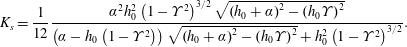 $$\begin{eqnarray}K_{s}={\displaystyle \frac{1}{12}}{\displaystyle \frac{\unicode[STIX]{x1D6FC}^{2}h_{0}^{2}\left(1-\unicode[STIX]{x1D6F6}^{2}\right)^{3/2}\sqrt{\left(h_{0}+\unicode[STIX]{x1D6FC}\right)^{2}-\left(h_{0}\unicode[STIX]{x1D6F6}\right)^{2}}}{\left(\unicode[STIX]{x1D6FC}-h_{0}\left(1-\unicode[STIX]{x1D6F6}^{2}\right)\right)\sqrt{\left(h_{0}+\unicode[STIX]{x1D6FC}\right)^{2}-\left(h_{0}\unicode[STIX]{x1D6F6}\right)^{2}}+h_{0}^{2}\left(1-\unicode[STIX]{x1D6F6}^{2}\right)^{3/2}}}.\end{eqnarray}$$
In the limiting case of no-slip flow, the intrinsic transmissivity for the parallel configuration is
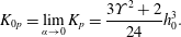 $$\begin{eqnarray}K_{0p}=\lim _{\unicode[STIX]{x1D6FC}\rightarrow 0}K_{p}={\displaystyle \frac{3\unicode[STIX]{x1D6F6}^{2}+2}{24}}h_{0}^{3}.\end{eqnarray}$$
For the serial configuration, the use of l’Hôpital’s rule twice indicates that the transmissivity reduces to
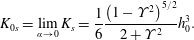 $$\begin{eqnarray}K_{0s}=\lim _{\unicode[STIX]{x1D6FC}\rightarrow 0}K_{s}={\displaystyle \frac{1}{6}}{\displaystyle \frac{\left(1-\unicode[STIX]{x1D6F6}^{2}\right)^{5/2}}{2+\unicode[STIX]{x1D6F6}^{2}}}h_{0}^{3}.\end{eqnarray}$$
These last two results coincide with those reported in a previous work in the case of an incompressible flow with a no-slip boundary condition, directly leading to the intrinsic transmissivities of a sinusoidal aperture field (Letalleur, Plouraboué & Prat Reference Letalleur, Plouraboué and Prat2002).
Exponential aperture field
In a second step, the following exponential aperture field is considered:
 $$\begin{eqnarray}h(x)=H\exp \left(-{\displaystyle \frac{\unicode[STIX]{x1D6F6}x}{l_{x}}}\right),\end{eqnarray}$$
where
 $\unicode[STIX]{x1D6F6}$
is a positive constant and
$\unicode[STIX]{x1D6F6}$
is a positive constant and
 $H$
is given by
$H$
is given by
 $$\begin{eqnarray}H={\displaystyle \frac{\unicode[STIX]{x1D6F6}h_{0}}{1-\text{e}^{-\unicode[STIX]{x1D6F6}}}}.\end{eqnarray}$$
In this case, the analytical results for the integrals in (4.1) and (4.2) yield the following expressions for
 $K_{p}$
and
$K_{p}$
and
 $K_{s}$
:
$K_{s}$
:
 $$\begin{eqnarray}\displaystyle & \displaystyle K_{p}={\displaystyle \frac{H^{3}}{36\unicode[STIX]{x1D6F6}}}\left(1-\text{e}^{-3\unicode[STIX]{x1D6F6}}\right)+{\displaystyle \frac{\unicode[STIX]{x1D6FC}H^{2}}{24\unicode[STIX]{x1D6F6}}}\left(1-\text{e}^{-2\unicode[STIX]{x1D6F6}}\right), & \displaystyle\end{eqnarray}$$
 $$\begin{eqnarray}\displaystyle & \displaystyle K_{s}={\displaystyle \frac{\unicode[STIX]{x1D6FC}^{3}H^{2}\unicode[STIX]{x1D6F6}}{6\left\{2H^{2}\ln \left({\displaystyle \frac{H+\unicode[STIX]{x1D6FC}\text{e}^{\unicode[STIX]{x1D6F6}}}{H+\unicode[STIX]{x1D6FC}}}\right)+2\unicode[STIX]{x1D6FC}H\left(1-\text{e}^{\unicode[STIX]{x1D6F6}}\right)-\unicode[STIX]{x1D6FC}^{2}\left(1-\text{e}^{2\unicode[STIX]{x1D6F6}}\right)\right\}}}. & \displaystyle\end{eqnarray}$$
Again, in the situation of no-slip flow, the intrinsic transmissivity of the exponential aperture field for the parallel configuration is recovered as
 $$\begin{eqnarray}K_{0p}=\lim _{\unicode[STIX]{x1D6FC}\rightarrow 0}K_{p}={\displaystyle \frac{H^{3}}{36\unicode[STIX]{x1D6F6}}}\left(1-\text{e}^{-3\unicode[STIX]{x1D6F6}}\right),\end{eqnarray}$$
whereas, for the serial configuration, it is given by
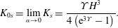 $$\begin{eqnarray}K_{0s}=\lim _{\unicode[STIX]{x1D6FC}\rightarrow 0}K_{s}={\displaystyle \frac{\unicode[STIX]{x1D6F6}H^{3}}{4\left(\text{e}^{3\unicode[STIX]{x1D6F6}}-1\right)}}.\end{eqnarray}$$
It must be noted that the transmissivity in the parallel configuration remains linear in
 $\unicode[STIX]{x1D6FC}$
(see (4.4) and (4.13)), while, conversely,
$\unicode[STIX]{x1D6FC}$
(see (4.4) and (4.13)), while, conversely,
 $K_{s}$
exhibits a nonlinear dependence on the slip parameter, as indicated by (4.8) and (4.14). This simply results from the fact that the linear dependence on the slip parameter at the local scale (see (2.28b
)) is preserved by the arithmetic mean while deriving
$K_{s}$
exhibits a nonlinear dependence on the slip parameter, as indicated by (4.8) and (4.14). This simply results from the fact that the linear dependence on the slip parameter at the local scale (see (2.28b
)) is preserved by the arithmetic mean while deriving
 $K_{p}$
, whereas the harmonic mean introduces nonlinearity. This further suggests that, in the general case, the macroscopic transmissivity tensor
$K_{p}$
, whereas the harmonic mean introduces nonlinearity. This further suggests that, in the general case, the macroscopic transmissivity tensor
 $\unicode[STIX]{x1D646}$
, which results from a complex average process reflected in (3.37), might not be linear in
$\unicode[STIX]{x1D646}$
, which results from a complex average process reflected in (3.37), might not be linear in
 $\unicode[STIX]{x1D709}\bar{\unicode[STIX]{x1D706}}$
. This will be further addressed in § 4.2.
$\unicode[STIX]{x1D709}\bar{\unicode[STIX]{x1D706}}$
. This will be further addressed in § 4.2.
The objective is now to compare the above analytical results for the macroscopic transmissivities of the sinusoidal and exponential aperture fields with those obtained from (3.37) and the numerical solution of the closure problem (3.33). The computed solution was achieved using a finite volume scheme over a regular grid, while the linear system deriving from the discretization process was solved using a preconditioned conjugate gradient algorithm (Moukalled, Mangani & Darwish Reference Moukalled, Mangani and Darwish2016). The numerical values of the parameters used for the sinusoidal and exponential aperture fields in our simulations are reported in table 1.
Table 1. Numerical values of the parameters used to define the sinusoidal and exponential aperture fields in (4.3) and (4.11) respectively. Three sets of parameters are investigated for each one. All variables are given in arbitrary but consistent units.
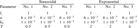
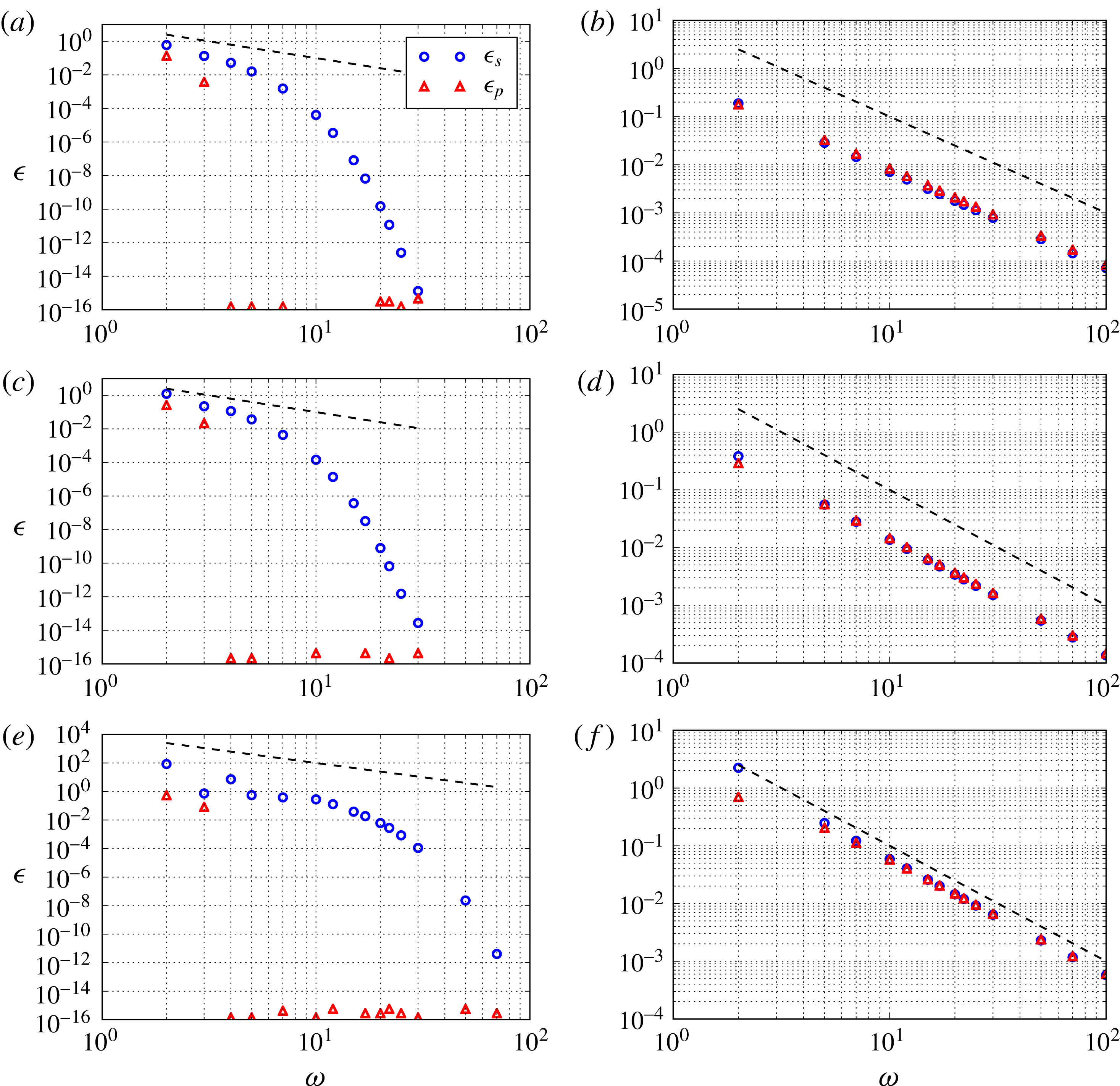
Figure 3. Variation of the relative error given in (4.17) between the analytical and numerical solutions versus the mesh density
 $\unicode[STIX]{x1D714}$
for the sinusoidal ((a) no. 1, (c) no. 2, (e) no. 3) and exponential ((b) no. 1, (d) no. 2, (f) no. 3) aperture fields. Parameters for aperture fields nos 1, 2 and 3 are provided in table 1. The dashed line represents a power law function of
$\unicode[STIX]{x1D714}$
for the sinusoidal ((a) no. 1, (c) no. 2, (e) no. 3) and exponential ((b) no. 1, (d) no. 2, (f) no. 3) aperture fields. Parameters for aperture fields nos 1, 2 and 3 are provided in table 1. The dashed line represents a power law function of
 $\unicode[STIX]{x1D714}$
with an exponent of
$\unicode[STIX]{x1D714}$
with an exponent of
 $-2$
.
$-2$
.
A quick analysis of the mesh convergence of the scheme must be carried out first to check the accuracy of the numerical procedure. Since the aperture fields under consideration only vary with respect to the
 $x$
coordinate, the computed macroscopic transmissivity tensor
$x$
coordinate, the computed macroscopic transmissivity tensor
 $\unicode[STIX]{x1D646}$
is diagonal, and the serial and parallel transmissivities correspond to the
$\unicode[STIX]{x1D646}$
is diagonal, and the serial and parallel transmissivities correspond to the
 $K_{xx}$
and
$K_{xx}$
and
 $K_{yy}$
components respectively. Convergence is hence analysed from the relative error between the computed and analytical solutions using the parameters
$K_{yy}$
components respectively. Convergence is hence analysed from the relative error between the computed and analytical solutions using the parameters
 $\unicode[STIX]{x1D716}_{p}$
and
$\unicode[STIX]{x1D716}_{p}$
and
 $\unicode[STIX]{x1D716}_{s}$
for the parallel and serial transmissivities, namely
$\unicode[STIX]{x1D716}_{s}$
for the parallel and serial transmissivities, namely
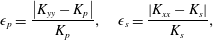 $$\begin{eqnarray}\displaystyle \unicode[STIX]{x1D716}_{p}={\displaystyle \frac{\left|K_{yy}-K_{p}\right|}{K_{p}}},\quad \unicode[STIX]{x1D716}_{s}={\displaystyle \frac{\left|K_{xx}-K_{s}\right|}{K_{s}}}, & & \displaystyle\end{eqnarray}$$
where
 $K_{p}$
and
$K_{p}$
and
 $K_{s}$
are respectively given by (4.4) and (4.8) for the sinusoidal fracture, and by (4.13) and (4.14) for the exponential aperture field.
$K_{s}$
are respectively given by (4.4) and (4.8) for the sinusoidal fracture, and by (4.13) and (4.14) for the exponential aperture field.
In figure 3, the variations of the relative errors
 $\unicode[STIX]{x1D716}_{s}$
and
$\unicode[STIX]{x1D716}_{s}$
and
 $\unicode[STIX]{x1D716}_{p}$
are reported versus the mesh density
$\unicode[STIX]{x1D716}_{p}$
are reported versus the mesh density
 $\unicode[STIX]{x1D714}$
, defined as the number of sampling points per unit length
$\unicode[STIX]{x1D714}$
, defined as the number of sampling points per unit length
 $l_{x}$
of the aperture field in the
$l_{x}$
of the aperture field in the
 $x$
-direction. The finite volume scheme employed in the numerical method is expected to be second-order-accurate in space (Moukalled et al.
Reference Moukalled, Mangani and Darwish2016). For the exponential aperture field, this property is clearly observed (see figure 3
b,d,f), whereas for the sinusoidal field, the scheme features a much faster convergence rate for both the serial and parallel transmissivities, as shown in figure 3(a,c,e), leading to the conclusion that the scheme is at least second-order-accurate in space.
$x$
-direction. The finite volume scheme employed in the numerical method is expected to be second-order-accurate in space (Moukalled et al.
Reference Moukalled, Mangani and Darwish2016). For the exponential aperture field, this property is clearly observed (see figure 3
b,d,f), whereas for the sinusoidal field, the scheme features a much faster convergence rate for both the serial and parallel transmissivities, as shown in figure 3(a,c,e), leading to the conclusion that the scheme is at least second-order-accurate in space.
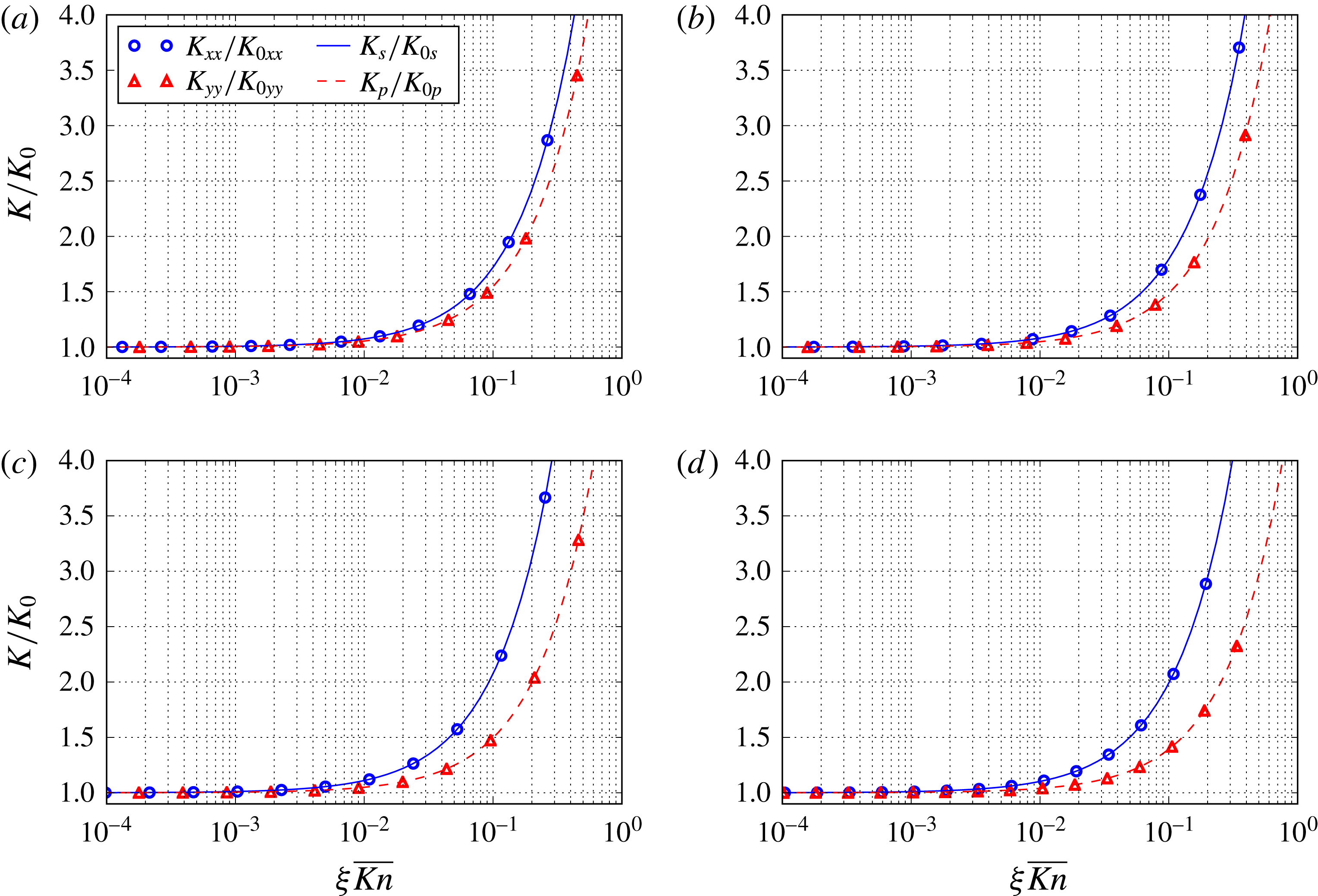
Figure 4. Ratio of the apparent slip-corrected to intrinsic transmissivity,
 $K_{ij}/K_{0ij}$
, as a function of
$K_{ij}/K_{0ij}$
, as a function of
 $\unicode[STIX]{x1D709}\overline{Kn}=\unicode[STIX]{x1D709}\bar{\unicode[STIX]{x1D706}}/h_{\unicode[STIX]{x1D6FD}j}$
for the sinusoidal fracture defined by (4.3) ((a) no. 1, (c) no. 3) and the exponential aperture field given in (4.11) ((b) no. 1, (d) no. 3) (see the parameters for aperture fields nos 1 and 3 in table 1). The characteristic aperture
$\unicode[STIX]{x1D709}\overline{Kn}=\unicode[STIX]{x1D709}\bar{\unicode[STIX]{x1D706}}/h_{\unicode[STIX]{x1D6FD}j}$
for the sinusoidal fracture defined by (4.3) ((a) no. 1, (c) no. 3) and the exponential aperture field given in (4.11) ((b) no. 1, (d) no. 3) (see the parameters for aperture fields nos 1 and 3 in table 1). The characteristic aperture
 $h_{\unicode[STIX]{x1D6FD}j}$
is defined by the relationship (4.18). Symbols represent the solutions computed from the closure problem (3.33) while lines are the analytical solutions reported in (4.4), (4.8) and (4.13), (4.14).
$h_{\unicode[STIX]{x1D6FD}j}$
is defined by the relationship (4.18). Symbols represent the solutions computed from the closure problem (3.33) while lines are the analytical solutions reported in (4.4), (4.8) and (4.13), (4.14).
We now report on the effect of the slip parameter on the transmissivities. Numerical results representing the ratio of the apparent slip-corrected to intrinsic transmissivity components,
 $K/K_{0}$
, versus
$K/K_{0}$
, versus
 $\unicode[STIX]{x1D709}\overline{Kn}=\unicode[STIX]{x1D709}\bar{\unicode[STIX]{x1D706}}/h_{\unicode[STIX]{x1D6FD}j}$
are represented in figure 4 for the sinusoidal and exponential aperture fields. Evidently, the normalized transmissivities exclusively depend on
$\unicode[STIX]{x1D709}\overline{Kn}=\unicode[STIX]{x1D709}\bar{\unicode[STIX]{x1D706}}/h_{\unicode[STIX]{x1D6FD}j}$
are represented in figure 4 for the sinusoidal and exponential aperture fields. Evidently, the normalized transmissivities exclusively depend on
 $\unicode[STIX]{x1D709}\overline{Kn}$
and
$\unicode[STIX]{x1D709}\overline{Kn}$
and
 $\unicode[STIX]{x1D6F6}$
, and, for this reason, results for aperture fields nos 1 and 3 only, characterized by contrasted values of
$\unicode[STIX]{x1D6F6}$
, and, for this reason, results for aperture fields nos 1 and 3 only, characterized by contrasted values of
 $\unicode[STIX]{x1D6F6}$
, are reported in figure 4. The Knudsen number was chosen to be characteristic of the flow direction by using
$\unicode[STIX]{x1D6F6}$
, are reported in figure 4. The Knudsen number was chosen to be characteristic of the flow direction by using
 $h_{\unicode[STIX]{x1D6FD}j}$
given by
$h_{\unicode[STIX]{x1D6FD}j}$
given by
 $$\begin{eqnarray}h_{\unicode[STIX]{x1D6FD}j}=\left(12K_{0jj}\right)^{1/3},\quad j=x,~y,\end{eqnarray}$$
which means that
 $h_{\unicode[STIX]{x1D6FD}j}$
represents the uniform aperture of a smooth fracture that would exhibit the same intrinsic transmissivity
$h_{\unicode[STIX]{x1D6FD}j}$
represents the uniform aperture of a smooth fracture that would exhibit the same intrinsic transmissivity
 $K_{0jj}$
in the
$K_{0jj}$
in the
 $j$
th direction (
$j$
th direction (
 $j=x,~y$
).
$j=x,~y$
).
The agreement of our numerical results with the analytical solutions of (4.4) and (4.8) for the two aperture fields under consideration is excellent over the whole range of
 $\unicode[STIX]{x1D709}\overline{Kn}$
. For all of the configurations (sinusoidal or exponential aperture fields, serial or parallel directions), the dependence of the normalized transmissivities on
$\unicode[STIX]{x1D709}\overline{Kn}$
. For all of the configurations (sinusoidal or exponential aperture fields, serial or parallel directions), the dependence of the normalized transmissivities on
 $\unicode[STIX]{x1D709}\overline{Kn}$
is quite similar, although the parallel normalized transmissivity remains smaller than the serial one in the whole range of
$\unicode[STIX]{x1D709}\overline{Kn}$
is quite similar, although the parallel normalized transmissivity remains smaller than the serial one in the whole range of
 $\unicode[STIX]{x1D709}\overline{Kn}$
. Moreover, one can notice that for both aperture fields, the serial normalized transmissivity increases while the parallel one decreases when
$\unicode[STIX]{x1D709}\overline{Kn}$
. Moreover, one can notice that for both aperture fields, the serial normalized transmissivity increases while the parallel one decreases when
 $\unicode[STIX]{x1D6F6}$
increases. This can be confirmed by a careful analysis of
$\unicode[STIX]{x1D6F6}$
increases. This can be confirmed by a careful analysis of
 $K_{p}/K_{0p}$
,
$K_{p}/K_{0p}$
,
 $K_{s}/K_{0s}$
obtained from the analytical expressions of the transmissivities given above. As expected, when the dimensionless slip parameter
$K_{s}/K_{0s}$
obtained from the analytical expressions of the transmissivities given above. As expected, when the dimensionless slip parameter
 $\unicode[STIX]{x1D709}\overline{Kn}$
tends to zero, all of the transmissivity components reach their corresponding intrinsic values as the flow occurs in the no-slip regime. These results assess the validity of the upscaled model and the numerical scheme used to solve the closure problem (3.33), allowing the determination of the macroscopic transmissivity tensor
$\unicode[STIX]{x1D709}\overline{Kn}$
tends to zero, all of the transmissivity components reach their corresponding intrinsic values as the flow occurs in the no-slip regime. These results assess the validity of the upscaled model and the numerical scheme used to solve the closure problem (3.33), allowing the determination of the macroscopic transmissivity tensor
 $\unicode[STIX]{x1D646}$
.
$\unicode[STIX]{x1D646}$
.
4.2 Solutions on a random Gaussian fracture
In this subsection, some illustrative results on the transmissivity obtained for the complete closure problem (3.33) to compute the tensor
 $\unicode[STIX]{x1D646}$
(see (3.37)) are presented. They are further compared with the first-order approximation in (3.48) derived from the solutions of the two subproblems (3.46) and (3.47) after decomposition, respectively yielding the complete form of the macroscopic transmissivity tensor
$\unicode[STIX]{x1D646}$
(see (3.37)) are presented. They are further compared with the first-order approximation in (3.48) derived from the solutions of the two subproblems (3.46) and (3.47) after decomposition, respectively yielding the complete form of the macroscopic transmissivity tensor
 $\unicode[STIX]{x1D646}$
defined by (3.37) and the decomposed one defined by relation (3.48). This is performed on a random Gaussian fracture.
$\unicode[STIX]{x1D646}$
defined by (3.37) and the decomposed one defined by relation (3.48). This is performed on a random Gaussian fracture.
4.2.1 Generation of the aperture field
The fracture aperture field considered in this section is generated from a random surface characterized by prescribed statistical parameters. As reported in many other works (see Mourzenko et al. (Reference Mourzenko, Thovert and Adler1995) and Plouraboué et al. (Reference Plouraboué, Fluckiger, Prat and Crispel2006) for instance), the surface height, denoted by
 $z$
, is supposed to obey a random shortly correlated Gaussian function. The numerical generation of the Gaussian rough surface was carried out with an algorithm proposed by Bergström (Reference Bergström2012) based on a methodology suggested by Garcia & Stoll (Reference Garcia and Stoll1984). The statistical distribution of
$z$
, is supposed to obey a random shortly correlated Gaussian function. The numerical generation of the Gaussian rough surface was carried out with an algorithm proposed by Bergström (Reference Bergström2012) based on a methodology suggested by Garcia & Stoll (Reference Garcia and Stoll1984). The statistical distribution of
 $z$
follows a Gaussian probability density function of zero mean value, given by
$z$
follows a Gaussian probability density function of zero mean value, given by
 $$\begin{eqnarray}\unicode[STIX]{x1D719}(z)={\displaystyle \frac{1}{\unicode[STIX]{x1D70E}_{h}\sqrt{2\unicode[STIX]{x03C0}}}}\exp \left(-{\displaystyle \frac{z^{2}}{2\unicode[STIX]{x1D70E}_{h}^{2}}}\right),\end{eqnarray}$$
in which
 $\unicode[STIX]{x1D70E}_{h}$
is the root mean square height of the surface.
$\unicode[STIX]{x1D70E}_{h}$
is the root mean square height of the surface.
To introduce a short-range correlation in both directions, the generated
 $z$
-field is convolved with a Gaussian filter so that the autocorrelation function
$z$
-field is convolved with a Gaussian filter so that the autocorrelation function
 $C\left(x,y\right)$
of the resulting surface height, which is also Gaussian for a Gaussian surface, is given by (Patir Reference Patir1978; Shi et al.
Reference Shi, Choi, Lowe, Skelton and Craster2015)
$C\left(x,y\right)$
of the resulting surface height, which is also Gaussian for a Gaussian surface, is given by (Patir Reference Patir1978; Shi et al.
Reference Shi, Choi, Lowe, Skelton and Craster2015)
 $$\begin{eqnarray}C(x,y)={\displaystyle \frac{\langle z(x_{0},y_{0})z(x_{0}+x,y_{0}+y)\rangle }{\unicode[STIX]{x1D70E}_{h}^{2}}}=\exp \left(-\left({\displaystyle \frac{x^{2}}{\unicode[STIX]{x1D70E}_{x}^{2}}}+{\displaystyle \frac{y^{2}}{\unicode[STIX]{x1D70E}_{y}^{2}}}\right)\right).\end{eqnarray}$$
In this expression,
 $\unicode[STIX]{x1D70E}_{x}$
and
$\unicode[STIX]{x1D70E}_{x}$
and
 $\unicode[STIX]{x1D70E}_{y}$
are the correlation lengths in the
$\unicode[STIX]{x1D70E}_{y}$
are the correlation lengths in the
 $x$
- and
$x$
- and
 $y$
-directions respectively. The surface dimensions in the
$y$
-directions respectively. The surface dimensions in the
 $x$
- and
$x$
- and
 $y$
-directions were set to
$y$
-directions were set to
 $l_{x}=l_{y}=1~\text{mm}$
and a
$l_{x}=l_{y}=1~\text{mm}$
and a
 $512\times 512$
Cartesian regular grid was used for the discretization. The root mean square height and correlation lengths were respectively taken as
$512\times 512$
Cartesian regular grid was used for the discretization. The root mean square height and correlation lengths were respectively taken as
 $\unicode[STIX]{x1D70E}_{h}=1.5~\unicode[STIX]{x03BC}\text{m}$
,
$\unicode[STIX]{x1D70E}_{h}=1.5~\unicode[STIX]{x03BC}\text{m}$
,
 $\unicode[STIX]{x1D70E}_{x}=40~\unicode[STIX]{x03BC}\text{m}$
and
$\unicode[STIX]{x1D70E}_{x}=40~\unicode[STIX]{x03BC}\text{m}$
and
 $\unicode[STIX]{x1D70E}_{y}=20~\unicode[STIX]{x03BC}\text{m}$
, so that the resulting surface was geometrically anisotropic. The final step to obtain the desired aperture field
$\unicode[STIX]{x1D70E}_{y}=20~\unicode[STIX]{x03BC}\text{m}$
, so that the resulting surface was geometrically anisotropic. The final step to obtain the desired aperture field
 $h(x,y)$
is to shift the generated Gaussian correlated surface
$h(x,y)$
is to shift the generated Gaussian correlated surface
 $z$
in the positive vertical direction by a value
$z$
in the positive vertical direction by a value
 $z_{0}$
(
$z_{0}$
(
 $z_{0}=2.2~\unicode[STIX]{x03BC}\text{m}$
) to obtain a new height field
$z_{0}=2.2~\unicode[STIX]{x03BC}\text{m}$
) to obtain a new height field
 $z^{\prime }=z+z_{0}$
. The aperture
$z^{\prime }=z+z_{0}$
. The aperture
 $h\left(x,y\right)$
is then given by
$h\left(x,y\right)$
is then given by
 $$\begin{eqnarray}h(x,y)=\left\{\begin{array}{@{}ll@{}}z^{\prime }(x,y),\quad & \text{if }z^{\prime }(x,y)>0,\\ 0,\quad & \text{if }z^{\prime }(x,y)\leqslant 0.\end{array}\right.\end{eqnarray}$$
A zero value of the aperture field corresponds to a contact spot in the fracture. The resulting generated aperture field is represented in figure 5.
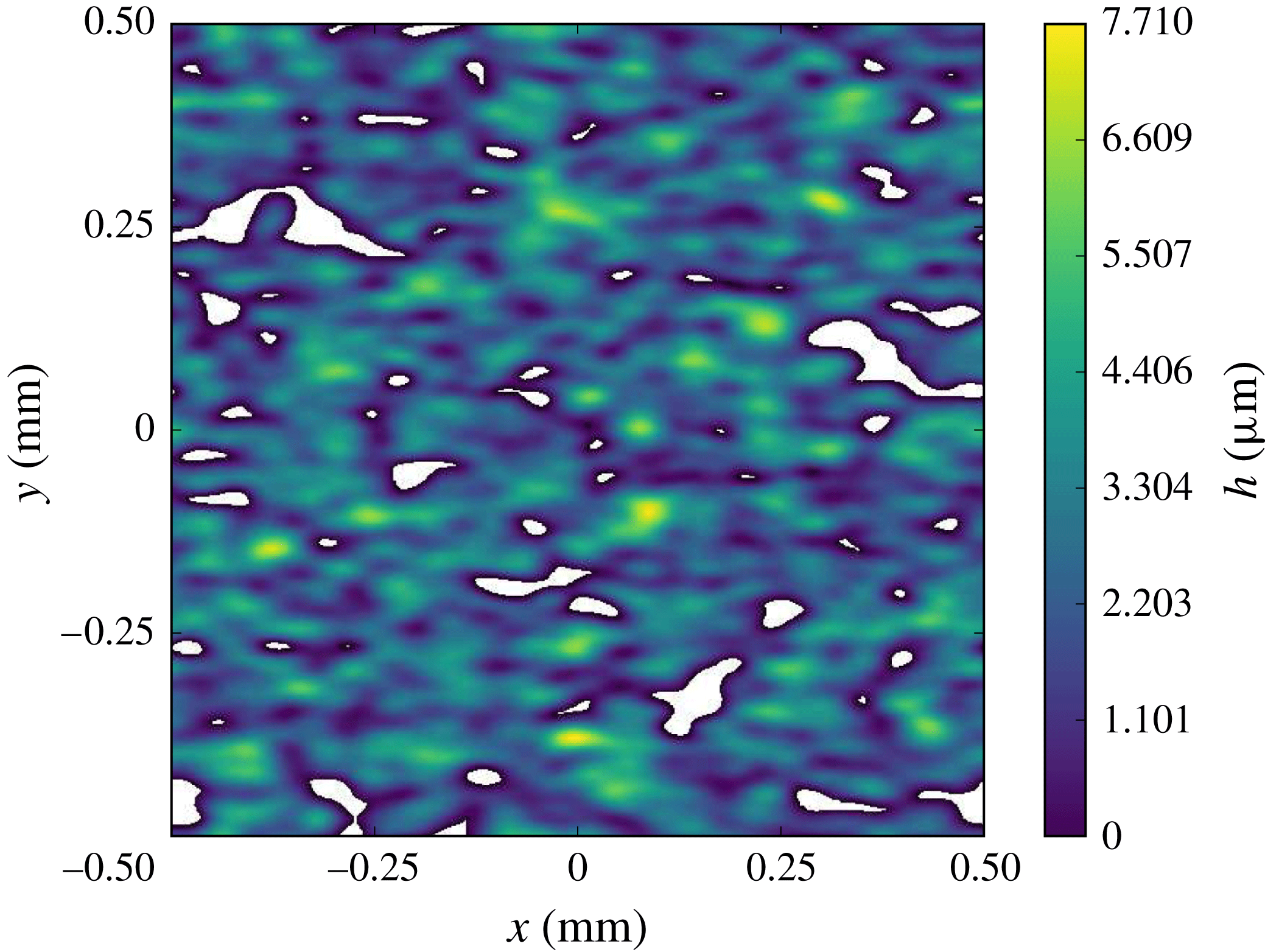
Figure 5. Numerically generated anisotropic aperture field. White zones denote contact spots (i.e. where
 $h(x,y)=0$
), so that the bearing area reaches
$h(x,y)=0$
), so that the bearing area reaches
 $7$
%.
$7$
%.
4.2.2 Closure solutions
The closure problem (3.33) was solved on the aperture field of figure 5. An example of the dimensionless fields of the closure variable
 $\boldsymbol{b}$
is reported in figure 6 with, for
$\boldsymbol{b}$
is reported in figure 6 with, for
 $\text{}\underline{b_{x}}$
,
$\text{}\underline{b_{x}}$
,
 $\unicode[STIX]{x1D709}\overline{Kn}=0.047$
, and, for
$\unicode[STIX]{x1D709}\overline{Kn}=0.047$
, and, for
 $\text{}\underline{b_{y}}$
,
$\text{}\underline{b_{y}}$
,
 $\unicode[STIX]{x1D709}\overline{Kn}=0.059$
. Again,
$\unicode[STIX]{x1D709}\overline{Kn}=0.059$
. Again,
 $\unicode[STIX]{x1D709}\overline{Kn}=\unicode[STIX]{x1D709}\bar{\unicode[STIX]{x1D706}}/h_{\unicode[STIX]{x1D6FD}j}$
,
$\unicode[STIX]{x1D709}\overline{Kn}=\unicode[STIX]{x1D709}\bar{\unicode[STIX]{x1D706}}/h_{\unicode[STIX]{x1D6FD}j}$
,
 $h_{\unicode[STIX]{x1D6FD}j}$
being given by the relationship (4.18). It should be noted that, since the aperture field is anisotropic with a preferential orientation of the roughness in the
$h_{\unicode[STIX]{x1D6FD}j}$
being given by the relationship (4.18). It should be noted that, since the aperture field is anisotropic with a preferential orientation of the roughness in the
 $x$
-direction (i.e.
$x$
-direction (i.e.
 $\unicode[STIX]{x1D70E}_{x}>\unicode[STIX]{x1D70E}_{y}$
), the value of
$\unicode[STIX]{x1D70E}_{x}>\unicode[STIX]{x1D70E}_{y}$
), the value of
 $K_{0xx}$
is expected to be larger than
$K_{0xx}$
is expected to be larger than
 $K_{0yy}$
, so that
$K_{0yy}$
, so that
 $\overline{Kn}$
is larger in the
$\overline{Kn}$
is larger in the
 $y$
-direction than in the
$y$
-direction than in the
 $x$
-direction. Physically, the closure variable fields represented in figure 6(a,b) are actually the pressure deviation fields made dimensionless by
$x$
-direction. Physically, the closure variable fields represented in figure 6(a,b) are actually the pressure deviation fields made dimensionless by
 $l_{j}\Vert \unicode[STIX]{x1D735}\langle p\rangle ^{\unicode[STIX]{x1D6FD}}\cdot \boldsymbol{e}_{j}\Vert ,j=x,~y$
, due to a unitary average-pressure gradient in the corresponding
$l_{j}\Vert \unicode[STIX]{x1D735}\langle p\rangle ^{\unicode[STIX]{x1D6FD}}\cdot \boldsymbol{e}_{j}\Vert ,j=x,~y$
, due to a unitary average-pressure gradient in the corresponding
 $j$
-direction.
$j$
-direction.
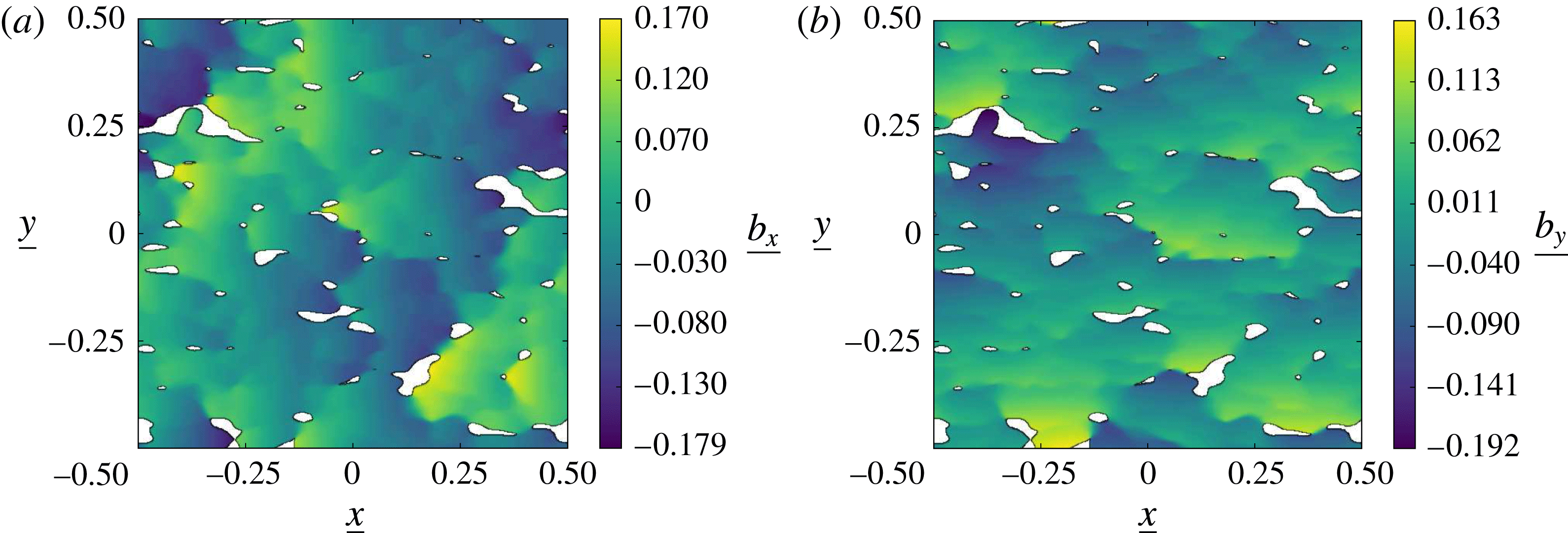
Figure 6. Dimensionless closure variable fields computed on the aperture field of figure 5: (a)
 $\text{}\underline{b_{x}}=b_{x}/l_{x}$
for
$\text{}\underline{b_{x}}=b_{x}/l_{x}$
for
 $\unicode[STIX]{x1D709}\overline{Kn}\approx 0.047$
; (b)
$\unicode[STIX]{x1D709}\overline{Kn}\approx 0.047$
; (b)
 $\text{}\underline{b_{y}}=b_{y}/l_{y}$
for
$\text{}\underline{b_{y}}=b_{y}/l_{y}$
for
 $\unicode[STIX]{x1D709}\overline{Kn}\approx 0.059$
. Surface dimensions are made dimensionless according to
$\unicode[STIX]{x1D709}\overline{Kn}\approx 0.059$
. Surface dimensions are made dimensionless according to
 $\text{}\underline{x}=x/l_{x}$
and
$\text{}\underline{x}=x/l_{x}$
and
 $\text{}\underline{y}=y/l_{y}$
.
$\text{}\underline{y}=y/l_{y}$
.
Similarly, the two closure subproblems (3.46) and (3.47) were solved sequentially using the same numerical procedure, the solution of the former being required to solve the latter. The dimensionless fields of the decomposed intrinsic closure variables
 $\boldsymbol{b}_{\mathbf{0}}$
and
$\boldsymbol{b}_{\mathbf{0}}$
and
 $\boldsymbol{b}_{\mathbf{1}}$
are represented in figure 7 for the aperture field of figure 5. All of the closure variable fields allow the computation of the transmissivity tensor
$\boldsymbol{b}_{\mathbf{1}}$
are represented in figure 7 for the aperture field of figure 5. All of the closure variable fields allow the computation of the transmissivity tensor
 $\unicode[STIX]{x1D646}$
and its approximation at
$\unicode[STIX]{x1D646}$
and its approximation at
 $O(\unicode[STIX]{x1D709}\overline{Kn})$
using the average in (3.37) and (3.48)–(3.50) respectively.
$O(\unicode[STIX]{x1D709}\overline{Kn})$
using the average in (3.37) and (3.48)–(3.50) respectively.
Results on the ratio of the apparent slip-corrected to intrinsic transmissivity components
 $K_{ij}/K_{0ij}$
(
$K_{ij}/K_{0ij}$
(
 $i,~j=x,~y$
) are represented versus
$i,~j=x,~y$
) are represented versus
 $\unicode[STIX]{x1D709}\overline{Kn}=\unicode[STIX]{x1D709}\bar{\unicode[STIX]{x1D706}}/h_{\unicode[STIX]{x1D6FD}j}$
in figure 8. It can be clearly seen that the apparent slip-corrected transmissivity exhibits a nonlinear behaviour with respect to
$\unicode[STIX]{x1D709}\overline{Kn}=\unicode[STIX]{x1D709}\bar{\unicode[STIX]{x1D706}}/h_{\unicode[STIX]{x1D6FD}j}$
in figure 8. It can be clearly seen that the apparent slip-corrected transmissivity exhibits a nonlinear behaviour with respect to
 $\unicode[STIX]{x1D709}\overline{Kn}$
, as indicated by the deviation of the complete transmissivity components from their first-order-approximation analogues. For the Gaussian aperture field under study in this section, a stronger nonlinearity is observed on the extra-diagonal terms of the transmissivity tensor compared with its diagonal components. The first-order approximation can therefore become inaccurate in some particular situations, even when
$\unicode[STIX]{x1D709}\overline{Kn}$
, as indicated by the deviation of the complete transmissivity components from their first-order-approximation analogues. For the Gaussian aperture field under study in this section, a stronger nonlinearity is observed on the extra-diagonal terms of the transmissivity tensor compared with its diagonal components. The first-order approximation can therefore become inaccurate in some particular situations, even when
 $\unicode[STIX]{x1D709}\overline{Kn}$
remains small enough for the slip regime to remain valid. To better illustrate this point, the relative error
$\unicode[STIX]{x1D709}\overline{Kn}$
remains small enough for the slip regime to remain valid. To better illustrate this point, the relative error
 $\unicode[STIX]{x1D716}$
between the complete apparent slip-corrected transmissivity and its first-order approximation is reported in figure 9. This figure shows that this relative error increases with increasing values of
$\unicode[STIX]{x1D716}$
between the complete apparent slip-corrected transmissivity and its first-order approximation is reported in figure 9. This figure shows that this relative error increases with increasing values of
 $\unicode[STIX]{x1D709}\overline{Kn}$
, whatever the component. Furthermore, for a given value of the slip parameter, this error is roughly one order of magnitude larger for the extra-diagonal terms than for the diagonal terms. For
$\unicode[STIX]{x1D709}\overline{Kn}$
, whatever the component. Furthermore, for a given value of the slip parameter, this error is roughly one order of magnitude larger for the extra-diagonal terms than for the diagonal terms. For
 $\unicode[STIX]{x1D709}\overline{Kn}\approx 0.1$
, the relative error is approximately
$\unicode[STIX]{x1D709}\overline{Kn}\approx 0.1$
, the relative error is approximately
 $1.5$
% for the diagonal terms and reaches
$1.5$
% for the diagonal terms and reaches
 $16$
% for the extra-diagonal terms. Consequently, the error cannot be considered as negligible even in a domain where the slip flow is expected to be relevant for this particular surface. As mentioned in § 4.1, this behaviour obviously results from the spatial dependence of the aperture field and from the averaging process which breaks the linearity present at the underlying roughness scale. In the particular case of a perfectly smooth fracture, the transmissivity tensor is spherical and depends linearly on
$16$
% for the extra-diagonal terms. Consequently, the error cannot be considered as negligible even in a domain where the slip flow is expected to be relevant for this particular surface. As mentioned in § 4.1, this behaviour obviously results from the spatial dependence of the aperture field and from the averaging process which breaks the linearity present at the underlying roughness scale. In the particular case of a perfectly smooth fracture, the transmissivity tensor is spherical and depends linearly on
 $\unicode[STIX]{x1D709}\overline{Kn}$
whatever its value, leading to a first-order approximation of the transmissivity tensor that exactly corresponds to the complete one.
$\unicode[STIX]{x1D709}\overline{Kn}$
whatever its value, leading to a first-order approximation of the transmissivity tensor that exactly corresponds to the complete one.
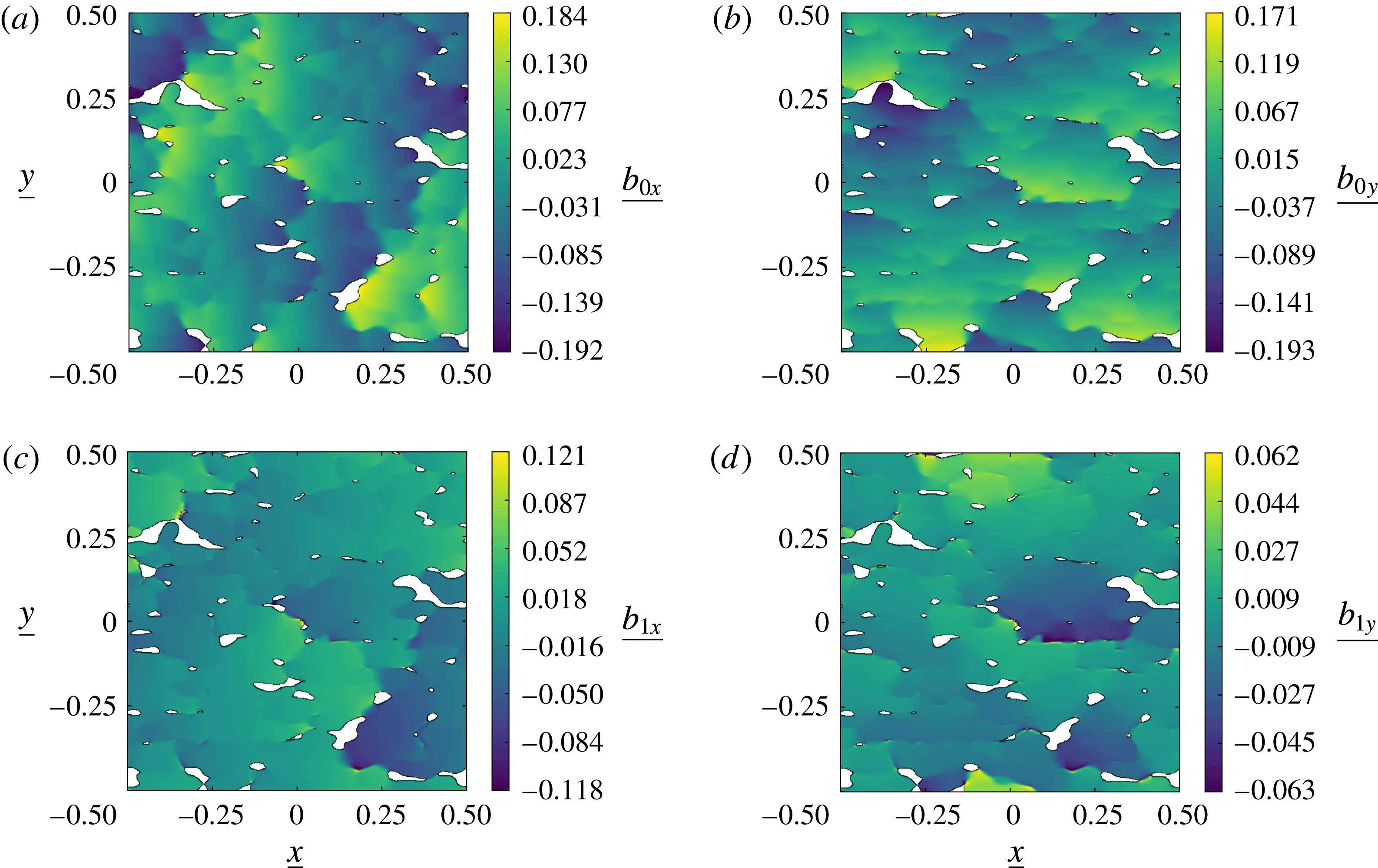
Figure 7. Dimensionless closure variable fields at the first order computed on the unit version of the aperture field of figure 5: (a)
 $\text{}\underline{b_{0x}}=b_{0x}/l_{x}$
; (b)
$\text{}\underline{b_{0x}}=b_{0x}/l_{x}$
; (b)
 $\text{}\underline{b_{0y}}=b_{0y}/l_{y}$
; (c)
$\text{}\underline{b_{0y}}=b_{0y}/l_{y}$
; (c)
 $\text{}\underline{b_{1x}}=b_{1x}h_{\unicode[STIX]{x1D6FD}x}/l_{x}$
; (d)
$\text{}\underline{b_{1x}}=b_{1x}h_{\unicode[STIX]{x1D6FD}x}/l_{x}$
; (d)
 $\text{}\underline{b_{1y}}=b_{1y}h_{\unicode[STIX]{x1D6FD}y}/l_{y}$
.
$\text{}\underline{b_{1y}}=b_{1y}h_{\unicode[STIX]{x1D6FD}y}/l_{y}$
.
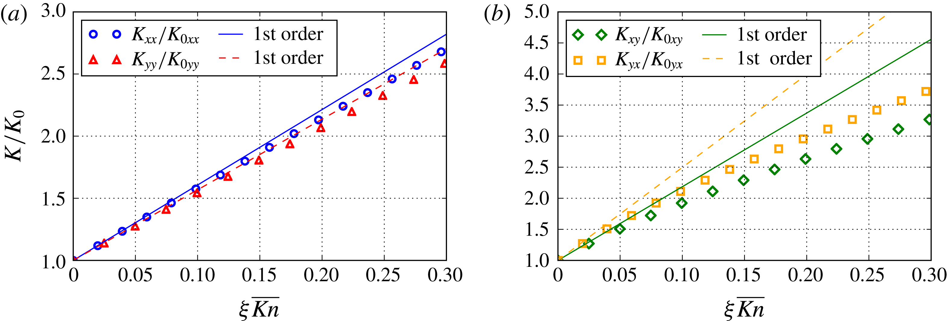
Figure 8. Ratio of the apparent slip-corrected to intrinsic transmissivity plotted as a function of the dimensionless slip parameter, computed from the solution of the complete closure problem (3.33) (symbols) and estimated at the first order with the solutions of the subproblems (3.46) and (3.47) (lines): (a) diagonal components; (b) extra-diagonal components.
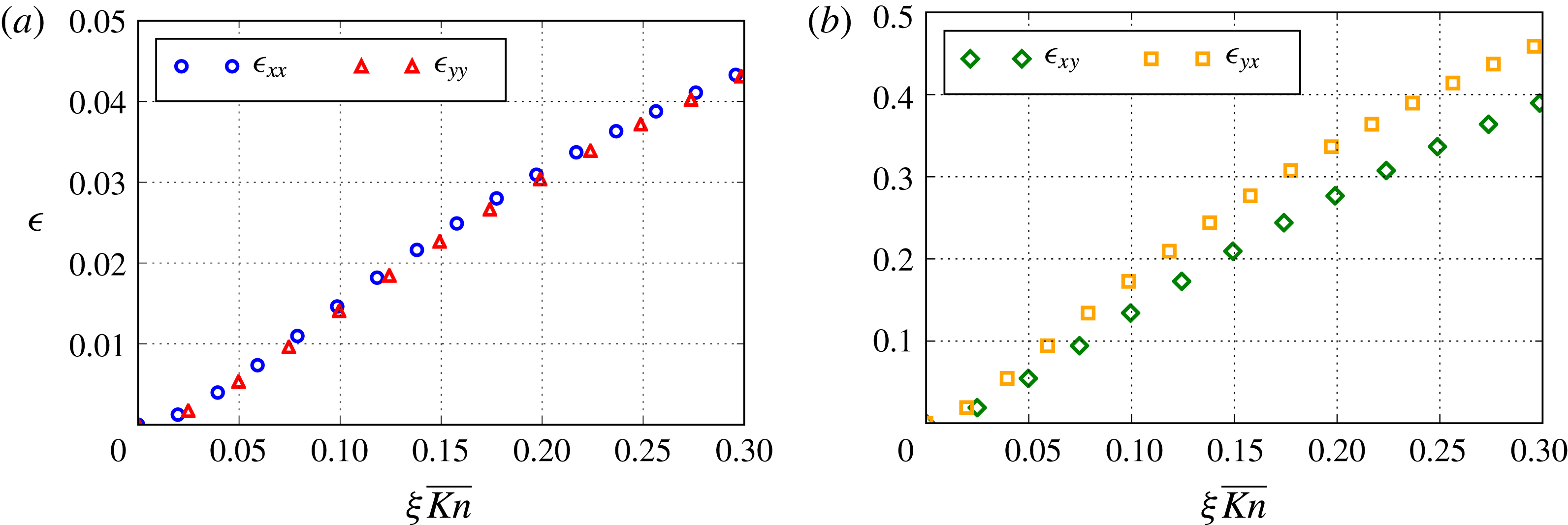
Figure 9. Evolution of the relative error between the computed solution of the complete closure problem (3.33) and estimated at the first order with the solutions of the subproblems (3.46) and (3.47). The solution of the complete closure problem is taken as the reference: (a) diagonal components; (b) extra-diagonal components.
5 Conclusions
In this work, a cautious formal derivation of the Reynolds equation for an isothermal slightly compressible gas flow in a fracture in the slip regime was derived first, using a first-order slip boundary condition at the fracture walls. The model is second-order-accurate in the local slope of the wall defaults and first-order-accurate in the Knudsen number at the roughness scale.
An upscaling procedure of the first-order slip-corrected Reynolds equation was applied next on an RES of a fracture using the method of volume averaging. As for any upscaling technique, the procedure was applied with the constraint that a scale hierarchy can be satisfied, an issue that must be carefully considered in the case of fractures in geological materials, for instance. In practice, however, this constraint might not be too restrictive regarding the first upscaling considered in this work, as, for instance, in the case of assemblies of machined surfaces. The ensuing upscaled model was shown to be entirely determined by the solution of a closure problem that is non-intrinsic due to the presence of slip. The derived macroscopic momentum conservation equation has a Reynolds-like form and involves an effective transmissivity tensor
 $\unicode[STIX]{x1D646}$
that is characteristic of the RES at a given Knudsen number. At the first order in the Knudsen number, the macroscopic transmissivity tensor can be approximated by an expansion that involves two intrinsic tensors, namely
$\unicode[STIX]{x1D646}$
that is characteristic of the RES at a given Knudsen number. At the first order in the Knudsen number, the macroscopic transmissivity tensor can be approximated by an expansion that involves two intrinsic tensors, namely
 $\unicode[STIX]{x1D646}_{\unicode[STIX]{x1D7EC}}$
, the purely viscous transmissivity tensor, and
$\unicode[STIX]{x1D646}_{\unicode[STIX]{x1D7EC}}$
, the purely viscous transmissivity tensor, and
 $\unicode[STIX]{x1D64E}$
, the slip-correction tensor, both being obtained from the solution of two coupled and intrinsic closure subproblems. When no-slip effect is considered in the model, the effective transmissivity tensor
$\unicode[STIX]{x1D64E}$
, the slip-correction tensor, both being obtained from the solution of two coupled and intrinsic closure subproblems. When no-slip effect is considered in the model, the effective transmissivity tensor
 $\unicode[STIX]{x1D646}$
and its first-order approximation both reduce to
$\unicode[STIX]{x1D646}$
and its first-order approximation both reduce to
 $\unicode[STIX]{x1D646}_{\unicode[STIX]{x1D7EC}}$
, in accordance with existing models (Prat et al.
Reference Prat, Plouraboué and Letalleur2002; Vallet et al.
Reference Vallet, Lasseux, Sainsot and Zahouani2009).
$\unicode[STIX]{x1D646}_{\unicode[STIX]{x1D7EC}}$
, in accordance with existing models (Prat et al.
Reference Prat, Plouraboué and Letalleur2002; Vallet et al.
Reference Vallet, Lasseux, Sainsot and Zahouani2009).
Validation of the complete non-intrinsic model was carried out numerically on fractures having simple geometries featuring defaults in one direction only, namely a sinusoidal and an exponential roughness, for which analytical expressions for the transmissivities with slip were obtained. The agreement between the analytical and computed solutions showed excellent agreement over the whole investigated range of the Knudsen number.
Numerical comparisons were performed between
 $\unicode[STIX]{x1D646}$
and its first-order approximation on a Gaussian shortly correlated rough aperture field. A nonlinear behaviour of the complete form of the transmissivity tensor was evidenced as a result of the averaging process which breaks the existing linearity at the underlying roughness scale. For this particular fracture, the relative error can reach non-negligible values for
$\unicode[STIX]{x1D646}$
and its first-order approximation on a Gaussian shortly correlated rough aperture field. A nonlinear behaviour of the complete form of the transmissivity tensor was evidenced as a result of the averaging process which breaks the existing linearity at the underlying roughness scale. For this particular fracture, the relative error can reach non-negligible values for
 $\unicode[STIX]{x1D709}\overline{Kn}\approx 0.1$
, especially for the off-diagonal terms of
$\unicode[STIX]{x1D709}\overline{Kn}\approx 0.1$
, especially for the off-diagonal terms of
 $\unicode[STIX]{x1D646}$
. Further work is necessary for an experimental validation of the upscaling procedure presented in this article.
$\unicode[STIX]{x1D646}$
. Further work is necessary for an experimental validation of the upscaling procedure presented in this article.
Acknowledgement
Financial support from CEA and CEA-Technetics joint sealing laboratory for this research is gratefully acknowledged.
Appendix A
In this appendix, it is shown that the arbitrary function
 $\unicode[STIX]{x1D6FE}$
involved in the representation of the pressure deviation (see (3.32)),
$\unicode[STIX]{x1D6FE}$
involved in the representation of the pressure deviation (see (3.32)),
 $$\begin{eqnarray}\widetilde{p}=\boldsymbol{b}\boldsymbol{\cdot }\unicode[STIX]{x1D735}\langle p\rangle ^{\unicode[STIX]{x1D6FD}}+\unicode[STIX]{x1D6FE},\end{eqnarray}$$
is a constant.
When this representation is inserted into the original closure problem given by (3.31), and taking into account that the closure vector
 $\boldsymbol{b}$
is chosen so as to satisfy the boundary-value problem (3.33), the following closure problem for
$\boldsymbol{b}$
is chosen so as to satisfy the boundary-value problem (3.33), the following closure problem for
 $\unicode[STIX]{x1D6FE}$
is obtained:
$\unicode[STIX]{x1D6FE}$
is obtained:
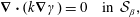 $$\begin{eqnarray}\displaystyle & \displaystyle \unicode[STIX]{x1D735}\boldsymbol{\cdot }\left(k\unicode[STIX]{x1D735}\unicode[STIX]{x1D6FE}\right)=0\quad \text{in }{\mathcal{S}}_{\unicode[STIX]{x1D6FD}}, & \displaystyle\end{eqnarray}$$
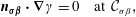 $$\begin{eqnarray}\displaystyle & \displaystyle \boldsymbol{n}_{\unicode[STIX]{x1D748}\unicode[STIX]{x1D737}}\boldsymbol{\cdot }\unicode[STIX]{x1D735}\unicode[STIX]{x1D6FE}=0\quad \text{at }{\mathcal{C}}_{\unicode[STIX]{x1D70E}\unicode[STIX]{x1D6FD}}, & \displaystyle\end{eqnarray}$$
 $$\begin{eqnarray}\displaystyle & \displaystyle \unicode[STIX]{x1D6FE}(\boldsymbol{x}+\unicode[STIX]{x1D72B}_{\boldsymbol{i}})=\unicode[STIX]{x1D6FE}(\boldsymbol{x}),\quad i=x,y. & \displaystyle\end{eqnarray}$$
By multiplying (A 2a
) by
 $\unicode[STIX]{x1D6FE}$
and rearranging the divergence, one obtains
$\unicode[STIX]{x1D6FE}$
and rearranging the divergence, one obtains
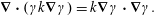 $$\begin{eqnarray}\unicode[STIX]{x1D735}\boldsymbol{\cdot }\left(\unicode[STIX]{x1D6FE}k\unicode[STIX]{x1D735}\unicode[STIX]{x1D6FE}\right)=k\unicode[STIX]{x1D735}\unicode[STIX]{x1D6FE}\boldsymbol{\cdot }\unicode[STIX]{x1D735}\unicode[STIX]{x1D6FE}.\end{eqnarray}$$
This expression can now be integrated over
 ${\mathcal{S}}_{\unicode[STIX]{x1D6FD}}$
to give
${\mathcal{S}}_{\unicode[STIX]{x1D6FD}}$
to give
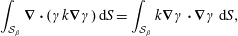 $$\begin{eqnarray}\int _{{\mathcal{S}}_{\unicode[STIX]{x1D6FD}}}^{}\unicode[STIX]{x1D735}\boldsymbol{\cdot }\left(\unicode[STIX]{x1D6FE}k\unicode[STIX]{x1D735}\unicode[STIX]{x1D6FE}\right)\,\text{d}S=\int _{{\mathcal{S}}_{\unicode[STIX]{x1D6FD}}}^{}k\unicode[STIX]{x1D735}\unicode[STIX]{x1D6FE}\boldsymbol{\cdot }\unicode[STIX]{x1D735}\unicode[STIX]{x1D6FE}\,\text{d}S,\end{eqnarray}$$
or, equivalently, when Ostrogradsky’s theorem is employed on the left-hand side of this expression,
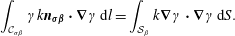 $$\begin{eqnarray}\int _{{\mathcal{C}}_{\unicode[STIX]{x1D70E}\unicode[STIX]{x1D6FD}}}^{}\unicode[STIX]{x1D6FE}k\boldsymbol{n}_{\unicode[STIX]{x1D748}\unicode[STIX]{x1D737}}\boldsymbol{\cdot }\unicode[STIX]{x1D735}\unicode[STIX]{x1D6FE}\,\text{d}l=\int _{{\mathcal{S}}_{\unicode[STIX]{x1D6FD}}}^{}k\unicode[STIX]{x1D735}\unicode[STIX]{x1D6FE}\boldsymbol{\cdot }\unicode[STIX]{x1D735}\unicode[STIX]{x1D6FE}\,\text{d}S.\end{eqnarray}$$
Use of the boundary condition (A 2b ) in (A 5) allows a simplification of the latter to the following form:
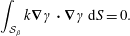 $$\begin{eqnarray}\int _{{\mathcal{S}}_{\unicode[STIX]{x1D6FD}}}^{}k\unicode[STIX]{x1D735}\unicode[STIX]{x1D6FE}\boldsymbol{\cdot }\unicode[STIX]{x1D735}\unicode[STIX]{x1D6FE}\,\text{d}S=0.\end{eqnarray}$$
Since
 $k$
is not zero in
$k$
is not zero in
 ${\mathcal{S}}_{\unicode[STIX]{x1D6FD}}$
and
${\mathcal{S}}_{\unicode[STIX]{x1D6FD}}$
and
 $\unicode[STIX]{x1D735}\unicode[STIX]{x1D6FE}\boldsymbol{\cdot }\unicode[STIX]{x1D735}\unicode[STIX]{x1D6FE}\geqslant 0$
, the only possible solution to satisfy (A 6) is for
$\unicode[STIX]{x1D735}\unicode[STIX]{x1D6FE}\boldsymbol{\cdot }\unicode[STIX]{x1D735}\unicode[STIX]{x1D6FE}\geqslant 0$
, the only possible solution to satisfy (A 6) is for
 $\unicode[STIX]{x1D6FE}$
to be a constant, completing the proof. Any constant superimposed on the field of
$\unicode[STIX]{x1D6FE}$
to be a constant, completing the proof. Any constant superimposed on the field of
 $\widetilde{p}$
is of no importance in the macroscopic model that involves
$\widetilde{p}$
is of no importance in the macroscopic model that involves
 $\unicode[STIX]{x1D735}\widetilde{p}$
in the closure procedure leading to the macroscopic Reynolds model.
$\unicode[STIX]{x1D735}\widetilde{p}$
in the closure procedure leading to the macroscopic Reynolds model.


