


1. Introduction
Understanding particle filtration and particle flocculation require an understanding of the hydrodynamic interactions of permeable particles and particles with a permeable medium (Belfort, Davis & Zydney Reference Belfort, Davis and Zydney1994; Le-Clech, Chen & Fane Reference Le-Clech, Chen and Fane2006; Civan Reference Civan2007; Hwang & Sz Reference Hwang and Sz2011; Wang et al. Reference Wang, Cahyadi, Wu, Pee, Fane and Chew2020). The operation and design of packed-bed and fluidized reactors (Rodrigues, Ahn & Zoulalian Reference Rodrigues, Ahn and Zoulalian1982; Davis & Stone Reference Davis and Stone1993) and chromatography columns (Liapis & McCoy Reference Liapis and McCoy1994; Blue & Jorgenson Reference Blue and Jorgenson2015) also relies on a fundamental understanding of the hydrodynamics of permeable particles.
Fluid flow in a homogeneous, permeable material is usually described using Darcy's law (Darcy Reference Darcy1856), whereby the fluid velocity  $\boldsymbol {v}$ in a permeable medium is given by
 \begin{equation} \boldsymbol{v}={-}\frac{k}{\mu}\boldsymbol{\nabla}p, \end{equation}
where  $k$ is the permeability,
  $\mu$ is the fluid viscosity and
  $\boldsymbol {\nabla }p$ is the local pressure gradient. The permeability scales with the square of the pore size and Darcy's law is appropriate when the length scale set by pressure gradients is much larger than the pore scale. The normal velocity and pressure are continuous at the boundary of a permeable material and the free fluid region. There have been several investigations of the appropriate boundary condition for the tangential velocity (Beavers & Joseph Reference Beavers and Joseph1967; Saffman Reference Saffman1971; Neale & Nader Reference Neale and Nader1974; Ochoa-Tapia & Whitaker Reference Ochoa-Tapia and Whitaker1995; Bars & Woster Reference Bars and Woster2006; Cao et al. Reference Cao, Gunzburger, Hua and Wang2010) but the no-slip boundary condition is most frequently used.
Brinkman's equation (Brinkman Reference Brinkman1949) is another widely used description of flows in permeable media. However, it is physically justified only for materials with very sparse microstructures, consisting of fixed arrays of particles (Tam Reference Tam1969; Childress Reference Childress1972; Howells Reference Howells1974; Lévy Reference Lévy1983), e.g. arrays of spheres with at least 95 % porosity (Durlofsky & Brady Reference Durlofsky and Brady1987). In any case, the ‘Brinkman term’ (i.e. Laplacian of the velocity) has an  $O(k/L^2)$ relative magnitude, where
  $L$ is the length scale associated with velocity gradients and
  $k^{1/2}$ is the pore scale. Accordingly, Brinkman's equation often reduces to Darcy's law, given that
  $L\gg k^{1/2}$ usually applies (Auriault Reference Auriault2009). As shown below, these conditions apply for the near-contact motion of permeable particles.
Hydrodynamic interactions between spherical particles and thin, permeable layers have been analysed as a model for filtration (Goren Reference Goren1979; Nir Reference Nir1981; Debbech, Elasmi & Feuillebois Reference Debbech, Elasmi and Feuillebois2010; Ramon & Hoek Reference Ramon and Hoek2012; Ramon et al. Reference Ramon, Huppert, Lister and Stone2013; Khabthani, Sellier & Feuillebois Reference Khabthani, Sellier and Feuillebois2019). Several studies explored the hydrodynamic interactions of spherical particles with permeable half-spaces (Michalopoulou, Burganos & Payatakes Reference Michalopoulou, Burganos and Payatakes1992; Damiano et al. Reference Damiano, Long, El-Khatib and Stace2004), conversely, others considered the interactions of permeable spheres with impermeable walls (Payatakes & Dassios Reference Payatakes and Dassios1987; Burganos et al. Reference Burganos, Michalopoulou, Dassios and Payatakes1992; Davis Reference Davis2001; Roy & Damiano Reference Roy and Damiano2008), and a few analysed hydrodynamic interactions between pairs of permeable spheres (Jones Reference Jones1978; Michalopoulou, Burganos & Payatakes Reference Michalopoulou, Burganos and Payatakes1993; Bäbler et al. Reference Bäbler, Sefcik, Morbidelli and Baldyga2006). Creeping flow conditions were assumed in all of these studies. Some used Darcy's law to describe the fluid flow in the permeable medium, others used Brinkman's equation (despite its limitations discussed above), the choice usually related to the porosity of the material (Auriault Reference Auriault2009). Most of the prior studies consider axisymmetric motion and the results show that permeability reduces hydrodynamic resistance (Goren Reference Goren1979; Nir Reference Nir1981; Payatakes & Dassios Reference Payatakes and Dassios1987; Burganos et al. Reference Burganos, Michalopoulou, Dassios and Payatakes1992; Michalopoulou et al. Reference Michalopoulou, Burganos and Payatakes1992, Reference Michalopoulou, Burganos and Payatakes1993; Davis Reference Davis2001; Debbech et al. Reference Debbech, Elasmi and Feuillebois2010; Ramon & Hoek Reference Ramon and Hoek2012; Ramon et al. Reference Ramon, Huppert, Lister and Stone2013; Khabthani et al. Reference Khabthani, Sellier and Feuillebois2019).
Much more is known about pairwise hydrodynamic interactions of hard spheres, i.e. impermeable rigid spheres, in creeping flows. Beginning with the classical study on axisymmetric pair interactions by Stimson & Jeffery (Reference Stimson and Jeffery1926), a complete formal framework was developed for pair interactions (Cooley & O'Neill Reference Cooley and O'Neill1969a; Lin, Lee & Sather Reference Lin, Lee and Sather1970; O'Neill & Majumdar Reference O'Neill and Majumdar1970a,Reference O'Neill and Majumdarb; Batchelor & Green Reference Batchelor and Green1972; Brenner & O'Neill Reference Brenner and O'Neill1972; Nir & Acrivos Reference Nir and Acrivos1973; Batchelor Reference Batchelor1982; Jeffrey Reference Jeffrey1982; Jeffrey & Onishi Reference Jeffrey and Onishi1984a,Reference Jeffrey and Onishib; Kim & Mifflin Reference Kim and Mifflin1985; Corless & Jeffrey Reference Corless and Jeffrey1988a,Reference Corless and Jeffreyb; Jeffrey Reference Jeffrey1989, Reference Jeffrey1992) with several additional studies on particle–wall interactions (Brenner Reference Brenner1961; Maude Reference Maude1963; Goldman, Cox & Brenner Reference Goldman, Cox and Brenner1967a,Reference Goldman, Cox and Brennerb; O'Neill & Stewartson Reference O'Neill and Stewartson1967; Cooley & O'Neill Reference Cooley and O'Neill1968). This work is summarized in classic texts (Happel & Brenner Reference Happel and Brenner1983; Kim & Karrila Reference Kim and Karrila2005). A principal result from this body of research is the general relationship between the forces, torques and stresslets acting on the particles and their linear and angular velocities and the imposed stress field by a grand resistance matrix that involves a set of scalar resistance functions that depend only on the centre-to-centre distance between particles (Kim & Karrila Reference Kim and Karrila2005).
Several methods have been used to compute the pairwise hydrodynamic resistances of hard spheres. Calculations using bispherical coordinates (Stimson & Jeffery Reference Stimson and Jeffery1926; Brenner Reference Brenner1961; Lin et al. Reference Lin, Lee and Sather1970; O'Neill & Majumdar Reference O'Neill and Majumdar1970a; Ingber & Zinchenko Reference Ingber and Zinchenko2012), twin-multipole expansions (Jeffrey & Onishi Reference Jeffrey and Onishi1984a,Reference Jeffrey and Onishib; Jeffrey Reference Jeffrey1992) and boundary collocation (Kim & Mifflin Reference Kim and Mifflin1985) provide exact results for all but near-contact configurations with vanishing surface-to-surface separation,  $h_0\to 0$, where the resistances are singular and these methods fail. The contact singularities of the resistance functions control important qualitative features of the hard-sphere dynamics. An example is the classical result that hard spheres cannot be pushed into contact by a finite force and thus interparticle contact does not occur in hard-sphere suspensions without singular interparticle forces (e.g. van der Waals attraction). Near-contact resistances must therefore be resolved, usually by a lubrication analysis (Goldman et al. Reference Goldman, Cox and Brenner1967a,Reference Goldman, Cox and Brennerb; O'Neill & Stewartson Reference O'Neill and Stewartson1967; Cooley & O'Neill Reference Cooley and O'Neill1968; O'Neill & Majumdar Reference O'Neill and Majumdar1970b; Jeffrey Reference Jeffrey1982; Corless & Jeffrey Reference Corless and Jeffrey1988a,Reference Corless and Jeffreyb; Jeffrey Reference Jeffrey1989).
The same methods have been applied to problems involving permeable particles and/or boundaries. Several studies on axisymmetric motion used bispherical coordinates calculations (Goren Reference Goren1979; Payatakes & Dassios Reference Payatakes and Dassios1987; Burganos et al. Reference Burganos, Michalopoulou, Dassios and Payatakes1992; Michalopoulou et al. Reference Michalopoulou, Burganos and Payatakes1992, Reference Michalopoulou, Burganos and Payatakes1993; Davis Reference Davis2001), and a few others used boundary collocation (Chen Reference Chen1998; Chen & Cai Reference Chen and Cai1999). Prior lubrication analyses have focused on the axisymmetric near-contact motion of hard spheres with permeable membranes. In a recent analysis of the near-contact motion between permeable spheres, we showed that the lubrication resistance between permeable particles is non-singular at contact, in contrast to the  $O(a/h_0)$ lubrication singularity that characterizes the relative motion of hard spheres (Reboucas & Loewenberg Reference Reboucas and Loewenberg2021a). This feature allows contact between particles in suspension, even without the presence of interparticle forces (Reboucas & Loewenberg Reference Reboucas and Loewenberg2021b).
Here, we extend our previous lubrication analysis (Reboucas & Loewenberg Reference Reboucas and Loewenberg2021a) to the case of asymmetric, transverse motion and use the general resistance framework for spherical particles (Kim & Karrila Reference Kim and Karrila2005) to derive the complete set of resistance functions that describe the near-contact motion of rigid, permeable spheres. The intraparticle flow is governed by Darcy's law, no-slip boundary conditions are applied on the particle surfaces and weak permeability conditions are assumed,
 \begin{equation} K\ll 1, \end{equation}
where  $K=k/a^2$ is the dimensionless permeability,
  $k$ is the arithmetic mean permeability of the particles,
 \begin{equation} k=\tfrac{1}{2}\left(k_1+k_2\right) \end{equation}
and  $a=a_1a_2(a_1+a_2)^{-1}$ is the reduced radius; subscripts 1 and 2 are particle labels. As discussed above, Brinkman's equation is inappropriate under weak permeability conditions. However, the use of Brinkman's equation would not significantly influence the results presented here because the length scale associated with the intraparticle velocity has the lower bound
  $L \geq k^{1/5} a^{3/5}$ (Reboucas & Loewenberg Reference Reboucas and Loewenberg2021a) thus, the Brinkman term has a sub-dominant,
  $O(K^{3/5})$, relative magnitude in Brinkman's equation (Auriault Reference Auriault2009).
Under weak permeability conditions (1.2), hydrodynamic resistances are sensitive to the permeability, and qualitatively affected, for gap widths  $h_0/a =O(K^{2/5})$, but at larger separations, particle permeability has a much weaker
  $O(K)$ effect on hydrodynamic resistances, allowing permeable particles to be approximated by hard spheres away from the near-contact region (Reboucas & Loewenberg Reference Reboucas and Loewenberg2021a). Thus, combining the lubrication resistances presented here with the resistances for well-separated hard spheres tabulated in the literature (Kim & Karrila Reference Kim and Karrila2005) provides a complete hydrodynamic description for pairwise hydrodynamic interactions of permeable spheres.
The governing lubrication equations are derived in § 2. An integral Reynolds lubrication equation that governs the pressure distribution is derived and solved numerically in § 3. The formulation allows for arbitrary ratios of particle radii and particles with different permeabilities. The resistance functions that describe the near-contact motion of permeable spheres are presented in § 4. Mobility functions, derived by combining the lubrication resistance functions for permeable spheres with the hard-sphere hydrodynamic functions for  $h_0/a\gg K^{2/5}$, are presented in § 5, including the special case of a particle undergoing near-contact translation parallel to a wall or a permeable half-space under the action of an applied force or an imposed shear flow. Concluding remarks are presented in § 6.
2. Problem formulation
The transverse motion of two permeable spheres separated by a small gap  $h_0$ in a fluid with viscosity
  $\mu$ is considered here. Particle 1 has radius
  $a_1$, particle 2 has radius
  $a_2$ and
  $\kappa =a_2/a_1$ will be used to denote the size ratio.
Note that various symbols have been used to denote size ratio in prior lubrication analyses, e.g.  $k^{-1}=\vert a_2/a_1\vert$ (O'Neill & Majumdar Reference O'Neill and Majumdar1970b),
  $\kappa =-a_1/a_2$ (Jeffrey Reference Jeffrey1982; Corless & Jeffrey Reference Corless and Jeffrey1988a,Reference Corless and Jeffreyb),
  $\lambda =a_2/a_1$ (Batchelor Reference Batchelor1982; Jeffrey & Onishi Reference Jeffrey and Onishi1984a; Jeffrey Reference Jeffrey1989, Reference Jeffrey1992) and
  $\beta =a_2/a_1$ (Kim & Karrila Reference Kim and Karrila2005). We use
  $\kappa =a_2/a_1$ here for consistency with our earlier study (Reboucas & Loewenberg Reference Reboucas and Loewenberg2021a).
2.1. Lubrication equations for transverse motions of permeable particles
A cylindrical coordinate system  $(r,\theta,z)$ is used with
  $z$-coordinate coincident with the line of centres of the two particles, and with
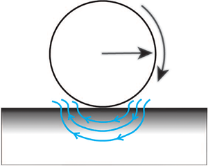
  $z=0$ at the surface of particle 2 shown in figure 1. A Cartesian coordinate system
  $(x,y,z)$ is also defined with the same origin,
  $x$-coordinate aligned with
  $\theta =0$, and
  $y$ aligned with
  $\theta ={\rm \pi} /2$. The surfaces of the particles are approximately parabolic in the near-contact region,
  $r\ll a$, where
  $a=a_1 a_2/(a_1+a_2)$ is the reduced radius. The surface of particle 1 corresponds to
  $z=h_0+r^2/(2 a_1)$, and the surface of particle 2 corresponds to
  $z=-r^2/(2 a_2)$.

Figure 1. Schematic showing two particles with radii and permeabilities  $a_i$ and
  $k_i$
$k_i$  $(i=1,2)$, respectively, separated by a gap
  $h_0$; particle 1 has translational and angular velocities
  $U_1$ and
  $\omega _1$; particle 2 is stationary. The Cartesian and cylindrical coordinate systems are shown.
The leading-order lubrication equations for transverse motion of the particles are
 \begin{equation} \frac{\partial^2 \bar v_r}{\partial \bar z^2}=\frac{\partial \bar p}{\partial \bar r},\quad \frac{\partial^2 \bar v_\theta}{\partial \bar z^2}=\frac{1}{\bar r}\frac{\partial \bar p}{\partial\theta},\quad \frac{\partial \bar p}{\partial \bar z}=0,\quad \frac{1}{\bar r}\frac{\partial }{\partial \bar r}\left(\bar r\bar v_r\right)+ \frac{1}{\bar r}\frac{\partial \bar v_\theta}{\partial\theta}+\frac{\partial \bar v_z}{\partial \bar z}=0. \end{equation}
The overbars denote dimensionless variables defined by
 \begin{equation} \bar r=\frac{r}{L_1},\quad \bar z=\frac{z a_1}{L_1^2},\quad \bar v_r=\frac{v_r}{U_0},\quad \bar v_\theta=\frac{v_\theta}{U_0},\quad \bar w=\frac{w a_1}{U_0 L_1},\quad \bar p=\frac{p L_1^3}{\mu U_0 a_1^2}, \end{equation}
where  $L_1=\sqrt {a_1 h_0}$ is the characteristic lateral length scale set by the geometry of the near-contact region, and
  $U_0$ is a characteristic velocity magnitude that depends on the boundary conditions of the problem. The lubrication approximation holds when
  $h_0\ll a$.
Only two transverse motions need consideration: (a) transverse motion of particle 1 with velocity in the  $x$-direction (i.e.
  $\theta =0$) with magnitude
  $U_1$, and (b) rotation of particle 1 with angular velocity in the positive
  $y$-direction with magnitude
  $\omega _1$. Particle 2 is stationary in both problems. The resistances corresponding to the translation and rotation of particle 2 are obtained by relabelling and symmetry. Boundary conditions for these two problems are
 \begin{gather} \bar z = \bar z_1(\bar r): \left\{\begin{array}{@{}l} \bar v_r=(\bar U_1-\bar \omega_1)\cos\theta,\quad \bar v_\theta={-}(\bar U_1-\bar \omega_1)\sin\theta \\ \bar v_z={-}\bar\omega_1 \bar r\cos\theta +\bar j_1[\bar p](\bar r,\theta) \end{array}\right., \end{gather}
 \begin{gather}\bar z= \bar z_2(\bar r):\quad \bar v_r=\bar v_\theta=0,\quad \bar v_z={-}\bar j_2[\bar p](\bar r,\theta), \end{gather}
where  $\bar z_1$ and
  $\bar z_2$ define the surfaces of particles 1 and 2, respectively,
 \begin{equation} \bar z_1=1+\frac{1}{2}\bar r^2,\quad \bar z_2={-}\frac{1}{2\kappa}\bar r^2. \end{equation}
Here,  $\bar U_1=U_1/U_0$ and
  $\bar \omega _1=\omega _1 a_1/U_0$ are the dimensionless translational and rotational velocities of particle 1. Recall that
  $\kappa =a_2/a_1$.
The quantities  $j_1, j_2$ are the fluxes of fluid into the surfaces of the permeable particles. Given that the intraparticle pressure fields satisfy Laplace's equation, are equal to the lubrication pressure at the particle surfaces, and decay to zero inside the particles, as shown in Appendix A, it follows that the intraparticle fluxes are linear functionals of the lubrication pressure. The intraparticle fluxes are normal to the particle surfaces but, as discussed in Appendix A, act in the
  $z$-direction to leading order, and thus only enter the boundary condition for the velocity in the
  $z$-direction, as indicated in (2.3)–(2.4). The fluxes are made dimensionless by the characteristic velocity in the
  $z$-direction,
  $U_0 L_1/a_1$,
 \begin{equation} \bar j_i=\frac{j_i a_1}{U_0 L_1}, \quad i=1,2. \end{equation}
 Boundary conditions (2.3)–(2.4) impose the following  $\theta$-dependence:
 \begin{gather} \bar v_r=\bar U(\bar r,\bar z)\cos\theta,\quad \bar v_\theta=\bar V(\bar r,\bar z)\sin\theta,\quad \bar v_z=\bar W(\bar r,\bar z)\cos\theta, \end{gather}
 \begin{gather}\bar p=\bar P(\bar r)\cos\theta,\quad \bar j_i=\bar J_i[\bar P](\bar r)\cos\theta,\quad i=1,2. \end{gather}
Inserting these forms into the lubrication equations (2.1a–d) and boundary conditions (2.3)–(2.4) yields,
 \begin{gather} \frac{\partial^2 \bar U}{\partial \bar z^2}=\bar P',\quad \frac{\partial^2 \bar V}{\partial \bar z^2}={-}\frac{\bar P}{\bar r}, \end{gather}
 \begin{gather} \frac{\partial \bar U}{\partial \bar r}+\frac{1}{\bar r}\left(\bar U+\bar V\right)+\frac{\partial \bar W}{\partial \bar z}=0, \end{gather}
 \begin{gather}\bar z=\bar z_1(\bar r): \left\{\begin{array}{@{}l} \bar U=(\bar U_1-\bar \omega_1),\quad \bar V={-}(\bar U_1-\bar \omega_1),\\ \bar W ={-}\bar \omega_1 \bar r +\bar J_1[\bar P](\bar r). \end{array}\right. \end{gather}
 \begin{gather}\bar z= \bar z_2(\bar r):\quad \bar U=\bar V=0,\quad \bar W={-}\bar J_2[P](\bar r). \end{gather}
Note that  $\bar P$ depends only on
  $\bar r$, and the prime in (2.8a,b) denotes a derivative.
Integrating the (2.8a,b) with boundary conditions (2.10)–(2.11) for  $\bar U$ and
  $\bar V$ yields
 \begin{gather} \bar U=\frac{1}{2}\bar P'(\bar r)(\bar z-\bar z_1(\bar r))(\bar z-\bar z_2(\bar r))+\frac{\bar U_1-\bar \omega_1}{\bar h(\bar r)}(\bar z-\bar z_2(\bar r)), \end{gather}
 \begin{gather}\bar V={-}\frac{1}{2\bar r}\bar P(\bar r)(\bar z-\bar z_1(\bar r))(\bar z-\bar z_2(\bar r))-\frac{\bar U_1-\bar \omega_1}{\bar h(\bar r)}(\bar z-\bar z_2(\bar r)), \end{gather}
where
 \begin{equation} \bar h(\bar r)=\bar z_{1}-\bar z_{2}=1+\tfrac{1}{2}(1+\kappa^{{-}1})\bar r^2. \end{equation}
 Inserting these results into the continuity equation (2.9) and integrating using the boundary conditions for  $\bar W$, yields the Reynolds lubrication equation
 \begin{equation} \frac{1}{12\bar r}\left(\bar r \bar P'\bar h^3\right)' -\frac{1}{12\bar r^2}\bar P \bar h^3-2\bar J\left[\bar P\right]={-}\frac{1}{2}C\left(1+\kappa^{{-}1}\right)\bar r, \end{equation}
which satisfies the homogeneous boundary conditions
 \begin{equation} \bar P(0)=\bar P(\infty)=0. \end{equation}
Here, primes are used to denote differentiation with respect to  $\bar r$ and
  $C$ is the constant
 \begin{equation} C=\left[\left(\bar U_1+\bar \omega_1\right)-\kappa^{{-}1}\left(\bar U_1-\bar \omega_1\right)\right] \left(1+\kappa^{{-}1}\right)^{{-}1}. \end{equation}
The quantity  $2\bar J=\bar J_1+\bar J_2$ is the combined flux into both particles. For hard spheres, i.e.
  $\bar J=0$, the solution of (2.14) is
 \begin{equation} \bar P_{\infty}(\kappa,\bar r)=C\frac{6 }{5} \frac{\bar r}{\bar h^{2}}. \end{equation}
2.2. Forces, torques and stresslets
The forces, torques and stresslets on each of the spheres are calculated using the relations (O'Neill & Majumdar Reference O'Neill and Majumdar1970b; Corless & Jeffrey Reference Corless and Jeffrey1988b),
 \begin{gather} \frac{F_{x_1}}{{\rm \pi} \mu U_0 a_1}= \int^{\bar R_{0}}_{0} \left[-\bar P r + \left(\frac{\partial \bar V}{\partial \bar z}- \frac{\partial \bar U}{\partial \bar z}\right)_{\bar z=\bar z_{1}}\right] r \,{\rm d} r, \end{gather}
 \begin{gather}\frac{F_{x_2}}{{\rm \pi} \mu U_0 a_1}=\int^{\bar R_{0}}_{0} \left[-\bar P r \kappa^{{-}1} + \left(\frac{\partial \bar U}{\partial \bar z}-\frac{\partial \bar V}{\partial \bar z}\right)_{\bar z=\bar z_{2}}\right] r \,{\rm d} r, \end{gather}
 \begin{gather}\frac{T_{y_1}}{{\rm \pi} \mu U_0 a^{2}_{1}}=\int^{\bar R_{0}}_{0} \left(\frac{\partial \bar U}{\partial \bar z}-\frac{\partial \bar V}{\partial \bar z}\right)_{\bar z=\bar z_{1}} r \,{\rm d} r, \end{gather}
 \begin{gather}\frac{T_{y_2}}{{\rm \pi} \mu U_0 a^{2}_{1}}=\kappa\int^{\bar R_{0}}_{0} \left(\frac{\partial \bar U}{\partial \bar z}-\frac{\partial \bar V}{\partial \bar z}\right)_{\bar z=\bar z_{2}} r\,{\rm d} r, \end{gather}
 \begin{gather}\frac{S_{xz,1}}{{\rm \pi} \mu U_0 a^{2}_{1}}= \int^{\bar R_{0}}_{0} \left[\bar P r + \frac{1}{2}\left(\frac{\partial \bar U}{\partial \bar z}-\frac{\partial \bar V}{\partial \bar z}\right)_{\bar z=\bar z_{1}}\right] r\,{\rm d} r, \end{gather}
 \begin{gather}\frac{S_{xz,2}}{{\rm \pi} \mu U_0 a^{2}_{1}}= \int^{\bar R_{0}}_{0} \left[-\bar P r + \frac{\kappa}{2}\left(\frac{\partial \bar U}{\partial \bar z}-\frac{\partial \bar V}{\partial \bar z}\right)_{\bar z=\bar z_{2}}\right]r \,{\rm d} r, \end{gather}
where the upper limit of integration is  $\bar R_{0}=O(\sqrt {a_1/h_0})$, a precise definition is not required (O'Neill & Stewartson Reference O'Neill and Stewartson1967; Kim & Karrila Reference Kim and Karrila2005).
Inserting (2.12a,b) into (2.17)–(2.22) and integrating by parts to separate the pressure contributions yields
 \begin{gather} \frac{F_{x_1}}{{\rm \pi} \mu U_0 a_1}=\frac{1}{2} C \left(\kappa^{{-}1}-1\right) (I_1-I_K )-2 B I_2, \end{gather}
 \begin{gather}\frac{F_{x_2}}{{\rm \pi} \mu U_0 a_1}={-}\frac{1}{2} C \left(\kappa^{{-}1}-1\right) (I_1-I_K) + 2 B I_2, \end{gather}
 \begin{gather}\frac{T_{y_1}}{{\rm \pi} \mu U_0 a^{2}_{1}}={-}\frac{1}{2} C\left(1+\kappa^{{-}1}\right)(I_1-I_K) + 2 B I_2, \end{gather}
 \begin{gather}\frac{T_{y_2}}{{\rm \pi} \mu U_0 a^{2}_{1}}= \frac{1}{2}C \left(1+\kappa\right)(I_1-I_K) + 2 \kappa B I_2, \end{gather}
 \begin{gather}\frac{S_{xz,1}}{{\rm \pi} \mu U_0 a^{2}_{1}}=\frac{1}{4}C\left(3-\kappa^{{-}1}\right) (I_1-I_K) + B I_2, \end{gather}
 \begin{gather}\frac{S_{xz,2}}{{\rm \pi} \mu U_0 a^{2}_{1}}={-}\frac{1}{4}C(3-\kappa) (I_1-I_K) + \kappa B I_2, \end{gather}
where  $B$ is given by
 \begin{equation} B=\bar U_1-\bar \omega_1 \end{equation}
and  $C$ is defined by (2.15). Here, we define the integrals
 \begin{equation} I_1(\xi,\kappa,\bar R_{0})=\int^{\bar R_{0}}_{0} \bar{\mathcal{P}}_\infty r^2 \,{\rm d} r,\quad I_2(\xi,\kappa,\bar R_{0})=\int^{\bar R_{0}}_{0} \frac{r}{\bar h} \,{\rm d} r, \end{equation}
and
 \begin{equation} I_K(\xi,\kappa,K)=\int^{\infty}_{0} (\bar{\mathcal{P}}_\infty-\bar{\mathcal{P}}) r^2 \,{\rm d} r, \end{equation}
where  $\xi =h_0/\bar a$ is the gap normalized by the average radius, and
  $\kappa =a_2/a_1$ is the size ratio. Here,
  $\mathcal {P}$ is the rescaled pressure
 \begin{equation} P=C\mathcal{P}, \end{equation}
which is introduced for convenience in the solution of the Reynolds lubrication equation that follows below.
This rearrangement of (2.17)–(2.22) is useful because it isolates the influence of particle permeability. The integrals  $I_1$ and
  $I_2$ describe the dynamics of hard spheres; only the permeability integral,
  $I_K$, depends on the permeability. The upper limit for
  $I_K$ can be extended to infinity because
  $\bar {\mathcal {P} }_\infty -\bar {\mathcal {P}}$ decays sufficiently fast for
  $\bar r\to \infty$, indicating that permeability does not affect flow in the matching region.
3. Solution of the Reynolds equation
In this section, an integral equation is derived for the pressure that allows evaluation of the permeability integral,  $I_K$. Numerical and asymptotic limiting results are presented. As shown below, the permeability integral can be expressed in terms of a single-variable permeability function
 \begin{equation} I_K(\xi,\kappa, K)=\left(1+\kappa^{{-}1}\right)^{{-}2} g(q), \end{equation}
where the parameter  $q$ is defined
 \begin{equation} q=K^{{-}2/5}\frac{h_0}{a}. \end{equation}
Here,  $K$ is the dimensionless permeability,
 \begin{equation} K=k/a^2, \end{equation}
where  $k=\frac {1}{2}(k_1+k_2)$ is the mean permeability, and
  $a=a_1 a_2/(a_1+a_2)$ is the reduced radius.
To obtain the functional form (3.1), we rescale the lubrication equation (2.14) using the variables
 \begin{equation} \hat r=\frac{r}{L_0},\quad \hat z=\frac{z a}{L_0^2},\quad \hat P=\frac{p L_0^3}{\mu U_0 a^2},\quad \hat J=\frac{J a}{U_0 L_0}q^{5/2}, \end{equation}
where
 \begin{equation} L_0=\sqrt{a h_0}, \end{equation}
is the length scale set by the geometry of the near-contact region (2.13), and  $a$ is the reduced radius. The scaling for the particle flux is obtained using the order-of-magnitude estimate,
  $J\sim k p/\mu L_0$ where
  $p\sim \mu U_0 a^2/L_0^3$ is the magnitude of pressure in the near-contact region.
In terms of these variables, the Reynolds lubrication equation (2.14) transforms to a one-parameter equation, depending only on  $q$. The result is
 \begin{equation} \frac{1}{12 \hat r}\left(\hat r \hat{\mathcal{P}}'\hat h^3\right)'-\frac{1}{12\hat r^2}\hat{\mathcal{P}} \hat h^3-2 q^{{-}5/2}\hat J\left[\hat{\mathcal{P}} \right]={-}\frac{1}{2}\hat r, \end{equation}
with boundary conditions
 \begin{equation} \hat{\mathcal{P}}(0)=\hat{\mathcal{P}}(\infty)=0, \end{equation}
where
 \begin{equation} \hat h(\hat r)=1+\tfrac{1}{2}\hat r^2 \end{equation}
is the gap profile, and primes denote differentiation with respect to  $\hat r$.
As shown in Appendix A, the intraparticle flux depends only on the mean permeability (1.3) and is expressed as a boundary integral of the pressure distribution in the gap between the particles
 \begin{equation} \hat J[\hat{\mathcal{P}}](\hat r)={-}\int_{0}^{\infty} \hat w(r)\phi(r/\hat r)\,{\rm d} r, \end{equation}
where  $\hat w$ is defined by derivatives of the pressure
 \begin{equation} \hat w(\hat r)=\left[\frac{1}{\hat r}\left(\hat r\hat{\mathcal{P}} \right)' \right]', \end{equation}
and the Green's function,  $\phi (x)$, is given by (A15). Similar boundary integrals arise in analogous lubrication problems from other fields where a coupling exists between spheres in contact, or near contact, and intraparticle transport (Hertz Reference Hertz1882; Batchelor & O'Brien Reference Batchelor and O'Brien1977; Davis, Schonberg & Rallison Reference Davis, Schonberg and Rallison1989).
The integro-differential Reynolds equation (3.6a) can be reduced to the integral equation,
 \begin{equation} \tfrac{1}{12}\hat w \hat h^3 +\tfrac{1}{4}\left(\hat I_A\left[ \hat w\right]+ \hat I_B\left[ \hat w\right]\right)\hat h^2\hat r-2 q^{{-}5/2}\hat J\left[ \hat w\right]={-}\tfrac{1}{2}\hat r, \end{equation}
where boundary conditions (3.6a) are incorporated,  $\hat w$ is defined by (3.9) and
 \begin{equation} \hat I_A\left[ \hat w\right]={-}\frac{1}{2}\int_{\hat r}^\infty \hat w\,{\rm d} r,\quad \hat I_B\left[ \hat w\right]=\frac{1}{2}\int_0^{\hat r} \left(\frac{r}{\hat r}\right)^2 \hat w\,{\rm d} r. \end{equation}
The rescaled pressure is obtained as
 \begin{equation} \hat{\mathcal{P}}=\left(\hat I_A-\hat I_B\right)\hat r. \end{equation}
The permeability function (3.1) is given by
 \begin{equation} g(q)=\int^{\infty}_{0} (\hat{\mathcal{P}}_\infty-\hat{\mathcal{P}}) r^2 \,{\rm d} r, \end{equation}
which, after integration by parts, becomes
 \begin{equation} g(q)=\frac{1}{8}\int^{\infty}_{0} (\hat w_\infty-\hat w) r^4 \,{\rm d} r. \end{equation}
Here,  $\hat {\mathcal {P}}_{\infty }$ is the pressure for hard spheres (2.16)
 \begin{equation} \hat{\mathcal{P}}_{\infty}(\hat r)=\frac{6}{5}\frac{\hat r}{\hat h^{2}}\, , \end{equation}
and
 \begin{equation} \hat w_\infty(\hat r)=\hat w\left[\hat{\mathcal{P}}_\infty\right](\hat r)= \frac{12\hat r}{5}\frac{\hat r^2-4}{\hat h^4}. \end{equation}
3.1. Numerical method
Integral (3.10), was discretized on a set of  $N$ points using a uniform mesh
  $\hat r_i$, (
 $i=1,\ldots, N$) on the interval
  $0 \leq \hat r \leq \hat r_N$. An
  $N\times N$ system of equations was thus generated for the values
  $\hat w_i$ at each of the points
  $\hat r_i$ using a piecewise linear representation of
  $\hat w$. The non-singular integrals
  $\hat I_A$ and
  $\hat I_B$, respectively, yield upper and lower triangular matrices with elements evaluated by trapezoid-rule integration on the intervals between points. The matrix obtained by discretizing the flux integral (3.8) was obtained by analytically evaluating the log-singular portion of the Green's function (A20) on all intervals and evaluating the non-analytic remainder with adaptive Gaussian quadratures. This method yields
  $O(1/N^2)$ convergence, and the permeability function
  $g(q)$ was obtained to
  $O(1/N^3)$ accuracy by extrapolating for
  $N\to \infty$ using results from calculations with different numbers of points. The contributions to integrals from the region
  $\hat r_N\leq \hat r\leq \infty$ were approximately incorporated using
  $\hat w\approx \hat w_\infty$ for
  $\hat r>\hat r_N$ to accelerate the convergence for
  $\hat r_N\to \infty$. The system of equations were iteratively solved using a Gauss–Seidel scheme.
The numerical values provided in the Supplementary Material available at https://doi.org/10.1017/jfm.2022.171 were obtained from calculations with  $N\approx 400$ and
  $\hat r_N\approx 20$ and are accurate to 3 digits.
3.2. Numerical and asymptotic results for the permeability function  $g(q)$

Results for the permeability function  $g(q)$ are shown graphically in figure 2 and provided in tabular form in the Supplementary Material. The limiting behaviours for small and large
  $q$, derived in Appendix B, are
 \begin{equation} g(q)={-}\tfrac{12}{5}\log q+b_1+b_2 q + O(q^2),\quad q\ll 1, \end{equation}
with  $b_1\doteq -0.48$ and
  $b_2\doteq -1.5$, and
 \begin{equation} g(q)=c_1 q^{{-}5/2}+O\left(q^{{-}5}\right),\quad q\gg 1, \end{equation}
with  $c_1\doteq 2.12$. The results show that
  $g(q)>0$, indicating that permeability reduces the lubrication pressure between particles undergoing transverse near-contact motion, i.e.
  $\hat P_\infty > \hat P$ according to (3.13).

Figure 2. Transverse and axisymmetric permeability functions  $g(q)$ and
  $f(q)$, defined by (3.13) and (D5), respectively; numerical solutions (solid lines), asymptotic forms (3.17)–(3.18) and (D6)–(D7) (dashed lines). Tables of numerical values for
  $f(q)$ and
  $g(q)$ are provided in the Supplementary Material.
4. Lubrication resistance functions for permeable spheres
We present here the complete set of resistance functions for near-contact motion of permeable particles, and discuss the effect of permeability.
4.1. Transverse resistance functions
Rearranging (2.23)–(2.28) to isolate the type of motion yields the forces, torques and stresslets in terms of resistance functions. The notation and general definition of resistance functions used in the literature is followed (Jeffrey Reference Jeffrey1992; Kim & Karrila Reference Kim and Karrila2005). The results are
 \begin{gather} -\frac{F_{x_1}}{ {\rm \pi}\mu U_0 a_1}= 6 Y^{A}_{11} \bar U_1+4Y^{B}_{11} \bar \omega_1, \end{gather}
 \begin{gather}-\frac{F_{x_2}}{ {\rm \pi}\mu U_0 a_1}= 3(1+\kappa) Y^{A}_{21} \bar U_1+ (1+\kappa)^2 Y^{B}_{21} \bar \omega_1, \end{gather}
 \begin{gather}- \frac{T_{y_1}}{ {\rm \pi}\mu U_0 a^2_1}= 4 Y^{B}_{11} \bar U_1+8 Y^{C}_{11} \bar \omega_1, \end{gather}
 \begin{gather}-\frac{T_{y_2}}{{\rm \pi} \mu U_0 a^2_1}= (1+\kappa)^2 Y^{B}_{21} \bar U_1+ (1+\kappa)^3 Y^{C}_{21} \bar \omega_1, \end{gather}
 \begin{gather}- \frac{S_{xz,1}}{{\rm \pi} \mu U_0 a^{2}_{1}}={-}4 Y^{G}_{11} \bar U_1+ 8 Y^{H}_{11} \bar \omega_1, \end{gather}
and
 \begin{equation} - \frac{S_{xz,2}}{{\rm \pi} \mu U_0 a^{2}_{1}}={-} (1+\kappa)^2 Y^{G}_{21} \bar U_1+ (1+\kappa)^3 Y^{H}_{21}\bar \omega_1. \end{equation}
Here,  $Y^{R}_{\alpha \beta }(\xi,\kappa,q)$ are the transverse resistance functions, where the superscript
  $R$ refers to one of the resistance tensors
  $A, B, C, G$ or
  $H$ in the resistance matrix (C1), and subscripts
  $\alpha$ and
  $\beta$ refer to the particle labels 1 or 2. Using symmetry relations and the Lorentz reciprocal theorem, the grand resistance matrix can be derived from this set of resistance functions, as shown in Appendix C.
The transverse resistance functions are
 \begin{equation} Y^{R}_{\alpha \beta}(\xi,\kappa,q)= Y^{R,0}_{\alpha \beta}(\xi,\kappa)-g(q) \varUpsilon^{R}_{\alpha \beta}(\kappa)+O\left(\xi \log \xi^{{-}1}\right), \end{equation}
where  $Y^{R,0}_{\alpha \beta }$ are the hard-sphere resistance functions (C5)–(C14),
  $g(q)$ is the transverse permeability function (3.13) shown in figure 2 and
  $\varUpsilon ^{R}_{\alpha \beta }$ are the size-ratio-dependent coefficients given by
 \begin{gather} \varUpsilon^{A}_{11}=\frac{\kappa}{12}\frac{(1-\kappa)^2 }{(\kappa +1)^3},\quad \varUpsilon^{A}_{21}={-}\frac{\kappa}{6}\frac{(1-\kappa)^{2}}{(\kappa +1)^{4}}, \end{gather}
 \begin{gather}\varUpsilon^{B}_{11}={-}\frac{\kappa}{8}\frac{(1-\kappa )}{(\kappa +1)^2},\quad \varUpsilon^{B}_{21}=\frac{\kappa^2}{2}\frac{1-\kappa}{(\kappa +1)^4}, \end{gather}
 \begin{gather}\varUpsilon^{C}_{11}=\frac{\kappa}{16 (1+\kappa)},\quad \varUpsilon^{C}_{21}={-}\frac{ \kappa^2}{2 (1+\kappa)^4}, \end{gather}
 \begin{gather}\varUpsilon^{G}_{11}={-}\frac{(3\kappa-1)(1-\kappa) \kappa}{16 (1+\kappa)^3},\quad \varUpsilon^{G}_{21}=\frac{(3-\kappa)(1-\kappa) \kappa^2}{4 (1+\kappa)^5}, \end{gather}
 \begin{gather}\varUpsilon^{H}_{11}={-}\frac{\kappa}{32}\frac{3\kappa-1}{(1+\kappa)^2},\quad \varUpsilon^{H}_{21}=\frac{\kappa^2}{4}\frac{3-\kappa}{(1+\kappa)^5}. \end{gather}
Recall that  $\xi =h_0/\bar a$ is the gap normalized by the average radius,
  $\kappa =a_2/a_1$ is the size ratio and
  $q=K^{-2/5}h_0/a$ is the permeability parameter. The result (4.7) indicates that particle permeability additively affects the transverse resistance functions.
4.2. Axisymmetric resistance functions
The leading-order axisymmetric resistance functions are presented here using the results of our recent analysis (Reboucas & Loewenberg Reference Reboucas and Loewenberg2021a). Following the presentation in § 4.1, the forces, torques and stresslets are (Jeffrey Reference Jeffrey1992; Kim & Karrila Reference Kim and Karrila2005)
 \begin{gather} -\frac{F_{z_1}}{ {\rm \pi}\mu U_0 a_1}= 6 X^{A}_{11} \bar U_1,\quad -\frac{F_{z_2}}{ {\rm \pi}\mu U_0 a_1}= 3(1+\kappa) X^{A}_{21} \bar U_1, \end{gather}
 \begin{gather}- \frac{T_{z_1}}{ {\rm \pi}\mu U_0 a^2_1}= 8 \, X^{C}_{11} \bar \omega_1,\quad -\frac{T_{z_2}}{{\rm \pi} \mu U_0 a^2_1}= (1+\kappa)^3 \, X^{C}_{21} \bar \omega_1, \end{gather}
 \begin{gather}- \frac{S_{zz,1}}{{\rm \pi} \mu U_0 a^{2}_{1}}={-}4X^{G}_{11} \bar U_1,\quad - \frac{S_{zz,2}}{{\rm \pi} \mu U_0 a^{2}_{1}}={-} (1+\kappa)^2X^{G}_{21} \bar U_1, \end{gather}
where  $\bar U_1$ and
  $\bar \omega _1$ are translational and rotational velocities of particle 1 along the line of centres, in the
  $z$-direction. Here,
  $X^{R}_{\alpha \beta }(\xi,\kappa,q)$ are the axisymmetric resistance functions, the superscript
  $R$ refers to the resistance tensor
  $A, C$ or
  $G$ and subscripts
  $\alpha$ and
  $\beta$ are particle labels 1 or 2. The remaining resistance functions for the grand resistance matrix (C1) for axisymmetric motion are derived from this set of functions, as shown in Appendix C.
The leading-order, axisymmetric resistance functions are
 \begin{equation} X^{A}_{\alpha \beta}(\xi,\kappa,q)= X^{A,0}_{\alpha \beta}(\xi,\kappa)f(q),\quad X^{G}_{\alpha \beta}(\xi,\kappa,q)= X^{G,0}_{\alpha \beta}(\xi,\kappa)f(q), \end{equation}
where  $X^{A,0}_{\alpha \beta }$ and
  $X^{G,0}_{\alpha \beta }$ are the hard-sphere resistance functions (C15)–(C18), and
  $f(q)$ is the axisymmetric permeability function (D5) shown in figure 2. This function was recently analysed (Reboucas & Loewenberg Reference Reboucas and Loewenberg2021a), and its primary features are summarized in Appendix D.
Particle permeability is seen to have a multiplicative effect on the axisymmetric resistance functions, in contrast to its additive effect on the transverse functions. Axisymmetric rotation does not generate a lubrication pressure thus,  $X^{C}_{\alpha \beta }(\xi,\kappa,q)=X^{C,0}_{\alpha \beta }(\xi,\kappa )$.
4.3. Matching to the outer region
Away from the near-contact region, hard-sphere resistance functions describe pairwise hydrodynamic interactions for permeable spheres to  $O(K)$. According to (3.18) and (4.7) and (D7) and (4.16a,b), the resistance functions for permeable spheres presented in § 4.1–4.2 are equal to the corresponding hard-sphere functions in the overlapping region
 \begin{equation} K^{2/5} \ll \epsilon \ll 1, \end{equation}
for  $K\to 0$, where
  $\epsilon =h_0/a$ is the gap normalized by the reduced radius
  $a=a_1a_2/(a_1+a_2)$. Accordingly, the resistance functions for permeable spheres match asymptotically to the hard-sphere functions. This provides a uniformly valid approximation for the resistance functions
 \begin{equation} Z^R_{\alpha\beta}(\xi,\kappa,q)= Z^{R,0}_{\alpha\beta}(\xi,\kappa)+Z^R_{L\alpha\beta} (\xi,\kappa,q)-Z^{R,0}_{L\alpha\beta}(\xi,\kappa), \end{equation}
where  $Z^R_{\alpha \beta }$ is a pairwise resistance function for permeable spheres,
  $Z^{R,0}_{\alpha \beta }$ is the corresponding hard-sphere resistance function,
  $Z^{R,0}_{L\alpha \beta }$ is the lubrication approximation for the hard-sphere function and
  $Z^R_{L\alpha \beta }$ is the lubrication resistance function for permeable spheres, as developed in our study.
4.4. Non-singular particle motions
The qualitative effects of particle permeability on the lubrication resistances are discussed below. Permeability relieves the lubrication pressure in the near-contact region, as discussed at the end of § 3.2 and at the end of Appendix D. We show here that permeability qualitatively alters near-contact motion of particles and gives rise to additional non-singular contact motions that are inaccessible to hard spheres. For hard spheres, only rigid-body motions, i.e. pair translation and dumbbell rotation, and relative rotations about the symmetry axis are non-singular at contact. As a result of permeability, non-shearing motions of particles in contact also become non-singular. These include rolling without slip and axisymmetric approach.
4.4.1. Transverse motions
Particle permeability lessens the magnitude of the transverse lubrication function  $Y^{R}_{\alpha \beta }$ if the contributions
  $Y^{R,0}_{\alpha \beta }$,
  $\varUpsilon ^{R}_{\alpha \beta }$ in (4.7) have the same algebraic sign; the latter is determined by formulas (4.8a,b)–(4.10a,b) and (C5)–(C10). It is thus seen that permeable particles of unequal size have lower translational resistances,
  $Y^{A}_{11}$,
  $Y^{A}_{21}$; translational resistances for equal-size particles are unaffected by permeability. Permeability reduces the rotational resistance
  $Y^C_{11}$ of a particle spinning close to a stationary particle but it enhances the rotational coupling between the particles, increasing
  $Y^C_{21}$.
To generally explain the role of permeability in transverse particle motions, it is convenient to examine the forces, torques and stresslets given by (2.23)–(2.28). The effect of permeability depends on whether the contribution from the lubrication pressure,  $I_1-I_K$, reinforces or opposes the contribution from shearing motion of the particle surfaces,
  $I_2$; permeability reduces the magnitude of the former contribution, but has no effect on the latter. Accordingly, the net effect of particle permeability depends on the coefficients of
  $I_1-I_K$ and
  $I_2$ in (2.23)–(2.28).
The forces, torques and stresslets for the special case of particle motion prescribed by
 \begin{equation} (\kappa -1)\bar U_1 + (\kappa +1)\bar \omega_1=0,\quad \bar U_2=\bar \omega_2=0 \end{equation}
are unaffected by particle permeability because  $C=0$ in this case, according to (2.15), and thus the pressure contribution, associated with
  $I_1-I_K$, vanishes in (2.23)–(2.28). This result explains why the translational resistances for equal-size particles are unaffected by permeability.
Conversely, the shearing contribution vanishes in (2.23)–(2.28) for rolling motion of the particles without slip,
 \begin{equation} \bar U_1=\bar \omega_1=1,\quad \bar U_2=\bar \omega_2=0, \end{equation}
because  $B=0$, according to (2.29). The forces, torques, and stresslets in this case are due entirely to the pressure contribution
  $I_1-I_K$, and thus have reduced magnitudes for permeable particles. Moreover, rolling motion of permeable particles is non-singular at contact, as shown by combining (3.1), (3.17) and (C4a) to yield,
 \begin{equation} \lim_{\xi\to 0}\left(I_1-I_K\right)= \frac{24}{25}\left(1+\kappa^{{-}1}\right)^{{-}2}\log K^{{-}1}+C_0, \end{equation}
where  $C_0$ depends only on size ratio. Other rolling motions without slip (e.g. pure rotation;
  $-\kappa \bar \omega _2=\bar \omega _1=1$,
  $\bar U_1=\bar U_2=0$) are also non-singular, and can be generated by a superposition of (4.20a,b) with non-singular rigid-body translation and rotation.
4.4.2. Axisymmetric motions
Given the form of the axisymmetric resistances (C15)–(C18), and formula (D6), it follows that axisymmetric resistances (4.16a,b) have the limiting forms,
 \begin{equation} \lim_{\xi\to 0}X^{A}_{\alpha \beta}(\xi,\kappa,q)= \chi^{A}_{\alpha \beta}(\kappa)K^{{-}2/5},\quad \lim_{\xi\to 0}X^{G}_{\alpha \beta}(\xi,\kappa,q)= \chi^{G}_{\alpha \beta}(\kappa)K^{{-}2/5}, \end{equation}
where the functions  $\chi ^{A}_{\alpha \beta }(\kappa )$ and
  $\chi ^{G}_{\alpha \beta }(\kappa )$ depend only on the size ratio. The result demonstrates that the axisymmetric resistances for permeable particles are non-singular at contact in contrast to the
  $\xi ^{-1}$ singular resistances for hard spheres.
5. Mobility functions
Here, we present pairwise mobilities of permeable particles defined by the relative velocity of the particles  $\boldsymbol {U}_{12}=\boldsymbol {U}_2-\boldsymbol {U}_1$ under the actions of forces and an imposed flow (Batchelor & Green Reference Batchelor and Green1972; Batchelor Reference Batchelor1982)
 \begin{align} \boldsymbol{U}_{12} &= \left[G(s)\boldsymbol{\hat r}\boldsymbol{\hat r}+ H(s)\left(\boldsymbol{I}-\boldsymbol{\hat r}\boldsymbol{\hat r}\right)\right] \boldsymbol{\cdot}\boldsymbol{U}_{12, 0}^\infty \nonumber\\ &\quad +\left[L(s)\boldsymbol{\hat r}\boldsymbol{\hat r}+ M(s)\left(\boldsymbol{I}-\boldsymbol{\hat r}\boldsymbol{\hat r}\right)\right] \boldsymbol{\cdot}\boldsymbol{U}_{12, g}^{\infty}\nonumber\\ &\quad +\boldsymbol{E}_\infty\boldsymbol{\cdot}\boldsymbol{r} + \boldsymbol{\omega}_\infty\times \boldsymbol{r}-\left[A(s)\boldsymbol{\hat r}\boldsymbol{\hat r}+ B(s)\left(\boldsymbol{I}-\boldsymbol{\hat r}\boldsymbol{\hat r}\right)\right] \boldsymbol{\cdot}\boldsymbol{E}_\infty\boldsymbol{\cdot}\boldsymbol{r}. \end{align}
Here,  $\boldsymbol {r}=\boldsymbol {x}_2-\boldsymbol {x}_1$ is the vector between the particle centres,
  $\boldsymbol {\hat r}=\boldsymbol {r}/\vert \boldsymbol {r}\vert$ is a unit vector along the line of centres,
  $\boldsymbol {I}$ is the identity tensor and
  $s=\vert \boldsymbol {r}\vert /\bar a$ is the centre-to-centre separation normalized by the average radius,
  $\bar a=\frac {1}{2}(a_1+a_2)$. The quantities
  $\boldsymbol {E}_\infty$ and
  $\boldsymbol {\omega }_\infty$ are the imposed rate of strain and vorticity in the fluid, and
  $\boldsymbol {U}_{12, 0}^\infty$ and
  $\boldsymbol {U}_{12, g}^{\infty }$ are, respectively, the relative velocities in the absence of hydrodynamic interactions (i.e.
  $s\to \infty$) under the action of equal and opposite forces and under the action of gravity
 \begin{equation} \boldsymbol{U}_{12, 0}^\infty=\frac{\boldsymbol{F}_2-\boldsymbol{F}_1}{6{\rm \pi} \mu a},\quad \boldsymbol{U}_{12, g}^\infty=\frac{2\left(a_2^2\gamma-a_1^2\right){\rm \Delta}\rho_1 \boldsymbol{g}}{9 \mu}, \end{equation}
where  $\boldsymbol {F}_1=-\boldsymbol {F}_2$,
  $a$ is the reduced radius,
  $\boldsymbol {g}$ is the acceleration due to gravity,
  ${\rm \Delta} \rho _i=\rho _i-\rho$ is the difference between the density of particle
  $i$ (
$i$ ( $i=1,2$) and the density of the fluid and
 \begin{equation} \gamma=\frac{{\rm \Delta}\rho_2}{{\rm \Delta}\rho_1}, \end{equation}
is the ratio of particle density differences.
Equation (5.1) defines the pairwise axisymmetric and transverse mobility functions  $G,L,A$ and
  $H,M,B$, respectively. According to their definitions,
  $G, H, L$ and
  $M$ tend to unity at large separations, whereas
  $A$ and
  $B$ vanish for
  $s\to \infty$. The pair mobilities depend on the centre-to-centre separation,
  $s$, size ratio,
  $\kappa$, and permeability,
  $K$ (
$K$ ( $L$ and
  $M$ also depend on the density difference ratio,
  $\gamma$). For the weak permeability regime (1.2) considered herein, hard-sphere mobilities can be used outside of the near-contact region with
  $O(K)$ error.
The near-contact mobilities  $H, M, B$ for transverse motion were obtained by inverting the resistance matrix (C1). The near-contact axisymmetric mobility
  $G$ was similarly obtained, and mobilities
  $L$ and
  $A$ derived by an analysis of the contact forces between spheres migrating along their line of centres, as described in section § 5.2. Outside of the near-contact region, mobilities were calculated using a code based on a bispherical coordinate solution for hard spheres provided by A.Z. Zinchenko.
5.1. Transverse mobilities
The transverse mobilities  $H$,
$H$,  $M$ and
  $B$ have the near-contact form
 \begin{equation} \varLambda(\xi,\kappa, K) =\frac{\lambda_1+\lambda_2\log\xi^{{-}1} + \lambda_3\left[\log\xi^{{-}1}-\frac{5}{12}g(q)\right]\log\xi^{{-}1} + \lambda_6 g(q)}{\lambda_4+\lambda_5\log\xi^{{-}1} + \left[\log\xi^{{-}1}-\frac{5}{12}g(q)\right]\log\xi^{{-}1} +\lambda_7 g(q)}, \end{equation}
where  $\xi =h_0/\bar a$ is the gap normalized by the average radius, and
  $q=K^{-2/5}h_0/a$ is the permeability parameter. The coefficients
  $\lambda _i$ (
 $i=1\text {--}7$) depend only on the size ratio; numerical values for several size ratios are listed in tables 1–3.
Table 1. Coefficients of transverse mobility  $H$ given by (5.4).

Table 2. Coefficients of transverse mobility  $M$ (
$M$ ( $\gamma =1$) given by (5.4).

Table 3. Coefficients of transverse mobility  $B$ given by (5.4).

The results shown in figures 3–5 demonstrate that permeability quantitatively affects the transverse mobilities for  $\xi \lesssim O(K^{2/5})$, corresponding to
  $q=O(1)$, and has the largest effect for extreme size ratios. Particle permeability has no effect for equal-size particles, as seen in figures 3 and 5, because no lubrication pressure is generated by the motion, as discussed in § 4.4.1.

Figure 3. Transverse mobility functions  $H$ from exact solution for hard spheres using code from A. Z. Zinchenko (solid lines) and lubrication solutions for hard spheres,
  $K=0$, and permeable spheres,
  $K=10^{-7}$ (dashed lines) vs gap,
  $\xi$, for size ratios indicated. Lubrication solution for hard spheres appears as a continuation of the exact solution; the lubrication solution for permeable spheres deviates for
  $\xi \lesssim K^{2/5}$.

Figure 4. Same as figure 3, except for the transverse mobility function  $M$.
$M$.

Figure 5. Same as figure 3, except for the transverse mobility function  $B$.
$B$.
Figures 3–4 show that mobility functions  $H$ and
  $M$ for permeable particles are larger than for hard spheres, whereas the opposite is true for mobility function
  $B$, as shown in figure 5. These observations indicate that particle permeability diminishes the strength of hydrodynamic pair interactions in all cases, given that
  $H=M=1$ and
  $B=0$ in the absence of hydrodynamic interactions.
Inserting (3.17) into (5.4) and taking the limit as  $\xi \to 0$ yields the contact values of the transverse mobilities
 \begin{equation} \varLambda_c(\kappa, K) =\lambda_3\frac{\log K^{{-}1}+\lambda'_1}{\log K^{{-}1}+\lambda'_2},\quad \xi=0, \end{equation}
where  $\varLambda _c$ is the contact value of the transverse mobility function
  $H$,
$H$,  $M$ or
  $B$, and the coefficients
  $\lambda '_1$ and
  $\lambda '_2$ are given by
 \begin{gather} \lambda'_1=6\lambda_6\lambda_3^{{-}1}+\tfrac{5}{2}\lambda_2\lambda_3^{{-}1}-\tfrac{5}{2} \log\nu-\tfrac{25}{24}b_1, \end{gather}
 \begin{gather}\lambda_2'=6\lambda_7+\tfrac{5}{2}\lambda_5-\tfrac{5}{2}\log\nu -\tfrac{25}{24}b_1, \end{gather}
where  $\nu =2\kappa (1+\kappa )^{-2}$ and
  $b_1\doteq -0.48$. For convenience, values for
  $\lambda _1'$ and
  $\lambda _2'$ are listed in table 4. Contact values for the mobilities of hard spheres are given by
  $\lambda _3$; even small permeabilities can significantly alter contact mobilities because its effect decays only logarithmically.
Table 4. Coefficients for the contact values of transverse mobilities given by (5.5).

According to formula (5.5),  $\varLambda _c$ increases with
  $K$ for
  $\lambda '_1>\lambda '_2$, decreases for
  $\lambda '_1<\lambda '_2$, the effect is largest for disparate values of these parameters, and
  $\varLambda _c$ is independent of
  $K$ for
  $\lambda '_1=\lambda '_2$. Consistent with the discussion above and the results shown in figures 3–5, the values in table 4 thus indicate that contact values of mobilities
  $H$ and
  $M$ increase with
  $K$,
$K$,  $B$ decreases with
  $K$, the effect is largest for extreme size ratios and
  $\varLambda _c$ is independent of
  $K$ for equal-size particles.
5.2. Axisymmetric mobilities
The axisymmetric mobility  $G$ has the near-contact form
 \begin{equation} G=\frac{(1+\kappa)^2}{2 \kappa} \frac{\xi}{f(q)}=\frac{\epsilon}{f(q)},\quad \xi\ll 1, \end{equation}
where  $\xi =h_0/\bar a$ and
  $\epsilon =h_0/a$ are the gaps normalized by the average and reduced radius, respectively,
  $\kappa$ is the size ratio and
  $q=K^{-2/5}h_0/a$ is the permeability parameter. Inserting (D6)–(D7) into (5.7) yields
 \begin{equation} G =\left(b_0+b_1 q+O(q^2)\right)K^{2/5},\quad q\ll 1, \end{equation}
and
 \begin{equation} G=\left(1+c_0 q^{{-}5/2}+O(q^{{-}5})\right)\epsilon,\quad q\gg 1, \end{equation}
where  $b_0\doteq 1.332$,
  $b_1\doteq 0.397$ and
  $c_0 \doteq 1.8402$. The result for hard spheres is recovered from the latter for
  $q\to \infty$. Equation (5.8) indicates that the particles undergo a constant approach velocity at contact under the action of a constant force, consistent with the non-singular axisymmetric resistances for permeable particles given by (4.22a,b).
In the near-contact region,  $L$ and
  $1-A$ are proportional to
  $G$, motivating the definition of modified mobility functions
  $\hat L$ and
  $\hat A_1$
 \begin{equation} \hat L(\epsilon,\kappa,q)=\frac{L(\epsilon,\kappa,q)}{\hat F_c^{(g)}(\kappa)},\quad \hat A_1(\epsilon,\kappa,q)=\frac{1-A(\epsilon,\kappa,q)}{\hat F_c^{(E)}(\kappa)}, \end{equation}
with the property
 \begin{equation} \lim_{\epsilon\to 0}\hat L(\epsilon,\kappa,q)= \lim_{\epsilon\to 0}\hat A_1(\epsilon,\kappa,q)= \lim_{\epsilon\to 0}G(\epsilon,q), \end{equation}
where  $\hat F_c^{(g)}$ and
  $\hat F_c^{(E)}$ are dimensionless contact forces, obtained by the procedure described in Appendix E and given by (E3)–(E4). These forces arise between two spheres in point contact, migrating along their line of centres in gravity-driven motion, and in axisymmetric straining flow, respectively. The mobility function
  $L$ also depends on the ratio of the particle density differences,
  $\gamma$, defined by (5.3). Numerical values of the contact forces are provided in table 6 for several size ratios.
Axisymmetric mobilities  $G, \hat L$ and
  $\hat A_1$ are shown in figure 6 as a function of gap where the common behaviour of the modified axisymmetric mobilities (5.11) is demonstrated; permeability qualitatively changes the near-contact motion for
  $h_0/a \leq O(K^{2/5})$, corresponding to
  $q\leq O(1)$. Figure 7 shows the universal near-contact behaviour predicted by combining (5.7) and (5.11)
 \begin{equation} G K^{{-}2/5}=\hat A_1 K^{{-}2/5}=\hat L K^{{-}2/5}=\frac{q}{f(q)},\quad \epsilon\to 0. \end{equation}
Figure 6. Axisymmetric mobility functions  $\hat A_1$ and
  $\hat L$ (
 $\gamma =1$), defined by (5.10a,b), and
  $G$ for hard spheres vs gap,
  $\epsilon =h_0/a$, for size ratios
  $\kappa =0.5$ (solid lines), and
  $\kappa =0.75$ (dash-dotted lines) using code from A. Z. Zinchenko (curves for
  $\kappa =0.5$, and
  $\kappa =0.75$ are indistinguishable for G); lubrication solution for hard spheres,
  $K=0$, and permeable spheres
  $K=10^{-7}$ (dashed lines).


5.3. Mobility of a particle moving parallel to a wall
In this section, the motion of a sphere in close contact with a wall is considered, corresponding to the limit  $\kappa \to \infty$. Two problems are studied: (I) motion of a particle in a quiescent fluid under the action of an imposed force
  $\boldsymbol {F}=F_0\boldsymbol {e}_x$ parallel to the wall and (II) motion of a force-free particle in an imposed shear flow parallel to the wall,
  $\boldsymbol {U}_{\infty }=E_\infty z \boldsymbol {e}_x$. The particle is torque free in both problems.
The resistance formulation for problems (I) and (II), derived from the general resistance formulation (C1) for the particle–wall configuration ( $\kappa \to \infty$), is
 \begin{gather} -\frac{F_{x_1}}{ {\rm \pi}\mu U_0 a_1}= 6 Y^{A,\infty}_{11} \bar U_1+4 Y^{B,\infty}_{11} \bar \omega_1 - (6 Y^{A,\infty}_{11}+2Y^{B,\infty}_{11}-4 Y^{G,\infty}_{11})\bar E_{\infty}, \end{gather}
 \begin{gather}- \frac{T_{y_1}}{ {\rm \pi}\mu U_0 a^2_1}= 4 Y^{B,\infty}_{11} \bar U_1+8 Y^{C,\infty}_{11} \bar \omega_1 -(4 Y^{B,\infty}_{11}+4Y^{C,\infty}_{11}+8 Y^{H,\infty}_{11})\bar E_{\infty}, \end{gather}
where  $a_1$ is the radius of the sphere,
  $\bar U_1=U_1/U_0$ and
  $\bar \omega _1=\omega _1 a_1/U_0$ are the dimensionless translational and rotational velocities,
  $\bar E_{\infty }=E_{\infty }a_1/U_0$ is the dimensionless shear rate and
  $Y^{R,\infty }_{11}$ are the resistance functions (4.7) corresponding to the limit
  $\kappa \to \infty$
 \begin{gather} Y^{A,\infty}_{11}={-}\frac{g(q)}{12}+\frac{8}{15}\log \epsilon^{{-}1} + A^{Y,\infty}_{11} + O(\epsilon \log \epsilon^{{-}1}), \end{gather}
 \begin{gather}Y^{B,\infty}_{11}={-}\frac{g(q)}{8}-\frac{1}{5}\log \epsilon^{{-}1} + B^{Y,\infty}_{11} + O(\epsilon \log \epsilon^{{-}1}), \end{gather}
 \begin{gather}Y^{C,\infty}_{11}={-}\frac{g(q)}{16}+\frac{2}{5}\log \epsilon^{{-}1} + C^{Y,\infty}_{11} + O(\epsilon \log \epsilon^{{-}1}). \end{gather}
 \begin{gather}Y^{G,\infty}_{11}={-}\frac{3}{16} g(q)+\frac{7}{10}\log \epsilon^{{-}1} + G^{Y,\infty}_{11} + O(\epsilon \log \epsilon^{{-}1}). \end{gather}
 \begin{gather}Y^{H,\infty}_{11}= \frac{3}{32} g(q)-\frac{1}{10}\log \epsilon^{{-}1} + H^{Y,\infty}_{11} + O(\epsilon \log \epsilon^{{-}1}). \end{gather}
Here,  $\epsilon =h_0/a_1$ is the dimensionless gap,
  $q=K^{-2/5}h_0/a_1$ is the permeability parameter,
  $g(q)$ is the transverse mobility function and
  $R^{Y,\infty }_{11}$ are the matching constants to the outer solution for this geometry (Goldman et al. Reference Goldman, Cox and Brenner1967a,Reference Goldman, Cox and Brennerb; Corless & Jeffrey Reference Corless and Jeffrey1988b).
The translational and rotational mobilities of the particle are determined by solving (5.13) and (5.14), separately, for problems (I) and (II). The results are
 \begin{equation} \bar{V}_1 =\frac{\lambda_0+\lambda_1\log\epsilon^{{-}1} +\lambda_2 g(q)}{\lambda_3+\lambda_4\log\epsilon^{{-}1} + \left[\log\epsilon^{{-}1}-\frac{5}{12}g(q)\right]\log\epsilon^{{-}1} +\lambda_5 g(q)}, \end{equation}
where  $\bar V_1=\bar U_1$ or
  $\bar V_1=\bar \omega _1$, and
  $U_0=(6 {\rm \pi}\mu a_1)^{-1}F_0$ for problem (I), and
  $U_0=E_{\infty }a_1$ for problem (II). The numerical coefficients appearing in (5.20) are listed in table 5 for both problems, and the results are plotted in figures 8 and 9. The results for hard spheres (Goldman et al. Reference Goldman, Cox and Brenner1967a,Reference Goldman, Cox and Brennerb; Corless & Jeffrey Reference Corless and Jeffrey1988b) are recovered for
  $g=0$, corresponding to
  $q\to \infty$.
Table 5. Coefficients for particle velocity parallel to wall (5.20).


Figure 9. Same as 8, except for a particle moving parallel to a plane wall in shear flow.
Inserting (3.17) into (5.20) yields a simplified analytical mobility formula depicted by the dashed lines in figures 8–9. Evaluating the result at contact yields
 \begin{equation} \bar U_1=\bar\omega_1=\frac{d_1}{\log K^{{-}1}+d_2}, \end{equation}
indicating that permeable particles roll without slipping. Here,  $d_1=3.125$,
  $d_1=7.280$ for problems (I), (II), respectively, and
  $d_2=6.666$ for both problems. This finding illustrates the non-singular rolling motion accessible to permeable particles at contact, as discussed in § 4.4. Hard spheres, by contrast, become stationary at contact and exhibit a slipping approach to contact with
  $\bar U_1>\bar \omega _1$ (Goldman et al. Reference Goldman, Cox and Brenner1967a,Reference Goldman, Cox and Brennerb), as seen in figures 8–9.
6. Conclusions
A lubrication analysis is presented for permeable, spherical particles using Darcy's law to describe the intraparticle velocity. Only the mean permeability enters the problem and the size ratio is arbitrary. The complete resistance matrix is derived for near-contact motions.
Under the weak permeability conditions (1.2) considered herein, particle permeability enters only in the lubrication regime, where it modifies the hydrodynamic resistances through the permeability functions,  $f(q)$ and
  $g(q)$, describing particle motions along and perpendicular to the line of centres, respectively, and
  $q=(h_0/a)K^{-2/5}$ is the permeability parameter. The permeability functions are obtained by solving an integral form of the Reynolds lubrication equation that results from the non-local coupling between the pressure in the gap and the intraparticle pressure. Outside of the near-contact region, the resistance functions can be approximated by hard-sphere functions and the two are equal in a finite matching region. Particle permeability removes the contact singularity for all non-shearing particle motions, allowing contacting permeable particles to roll without slipping and touching particles to separate with finite velocity.
Axisymmetric mobilities have a universal near-contact behaviour that depends only on the permeability parameter  $q$ and attain non-vanishing values at contact, proportional to
  $K^{2/5}$. Permeability enhances transverse mobilities, especially for extreme size ratios, but has no effect on equal-size particles because the relative particle motion in this case does not generate a lubrication pressure. Under the action of a constant force, or an imposed shear flow, a permeable particle in point contact with a planar boundary rolls with an
  $O(1/\log K^{-1})$ velocity, according to a formula derived herein. The same formula also describes a hard sphere rolling on a permeable half-space which may have relevance to cross-flow particle filtration.
Supplementary material
Supplementary material is available at https://doi.org/10.1017/jfm.2022.171.
Acknowledgements
The authors are grateful to Dr A.Z. Zinchenko for the use of his bispherical coordinate code for computing pair mobilities of hard spheres, and to Dr D.J. Jeffrey for the use of his program for resistance functions (https://www.uwo.ca/apmaths/faculty/jeffrey/) used herein to obtain the matching constants for the resistance functions of hard spheres.
Funding
This work was supported by the National Science Foundation (grant number 1603806) and the Coordenação de Aperfeiçoamento de Pessoal de Nível Superior - Brasil (Capes) (Finance Code 001).
Declaration of interests
The authors report no conflict of interest.
Appendix A. Derivation of intraparticle flux
In this appendix, we derive the combined intraparticle flux as a boundary integral of the pressure distribution in the near-contact region, given by formula (3.8) in the text. Unscaled, dimensional variables are used here. By Darcy's law (1.1) and the incompressibility of the fluid, the intraparticle pressure fields  $p_1$ and
  $p_2$ satisfy Laplace's equation. The combined intraparticle flux is
 \begin{equation} 2j=\frac{k_1}{\mu}\frac{\partial p_1}{\partial n}+\frac{k_2}{\mu}\frac{\partial p_2}{\partial n}, \end{equation}
where pressure gradients are evaluated on the particle surfaces, and  $\boldsymbol {n}$ is the outward normal vector. By continuity of pressure across the particle surfaces, the lateral lubrication length scale
  $L$ and angular dependence (2.7a) of the pressure distribution in the lubrication gap are imposed on the intraparticle pressure fields.
There are two length scales that can determine the lateral length scale of the lubrication region, the geometrically imposed length  $L_0$, given by equation (3.5), and
  $L_K$, a length scale set by the permeability (Reboucas & Loewenberg Reference Reboucas and Loewenberg2021a)
 \begin{equation} L_k=K^{1/5} a. \end{equation}
In this appendix,  $L$ is the maximum of these two length scales
 \begin{equation} L= \max(L_0, L_k), \end{equation}
and  $L/a\ll 1$ is assumed, where
  $a$ is the reduced radius.
As shown below, the intraparticle pressure fields decay to zero away from the near-contact region inside the particles on the length scale  $L$. A semi-infinite permeable region can thus be considered given that
  $L/a\ll 1$. A cylindrical coordinate system
  $(r,\theta, z)$ is used, where
  $z<0$ is the permeable region and
  $z>0$ is the fluid region. This is shown in figure 10. Normal derivatives of pressure on the particle boundary can be approximated by a
  $z$-derivative with error
  $O(L/a)^2$. Moreover, the intraparticle pressure fields are the same in each particle because they are forced only by the pressure distributions on their surfaces in the near-contact region, which are the same because pressure variations across the gap are negligible according to the leading-order lubrication equations (2.1a–d). Accordingly, (A1) simplifies to
 \begin{equation} j=\left. \frac{k}{\mu}\frac{\partial p_i}{\partial z}\right\vert_{z=0}, \end{equation}
where  $p_i$ denotes the intraparticle pressure. The result indicates that the total intraparticle flux depends only on the mean permeability (1.3).

Figure 10. Cylindrical coordinate system and orientation of normal vector  $\boldsymbol {n}$ used to describe pressure distribution in semi-infinite permeable region,
  $z<0$.
As discussed above, the intraparticle pressure field has the angular dependence
 \begin{equation} p_i(r,\theta,z)=P_i(r,z)\cos\theta, \end{equation}
imposed by continuity of the pressure at the particle–fluid interface, and it satisfies Laplace's equation. Hence,  $P_i(r,z)$ satisfies
 \begin{equation} \frac{1}{r}\frac{\partial}{\partial r}\left[\frac{1}{r} \frac{\partial}{\partial r} \left(r P_i\right)\right]+\frac{\partial^2 P_i}{\partial z^2}=0 \end{equation}
in the semi-infinite region shown in figure 10, vanishes for  $z\to -\infty$ and matches the pressure,
  $p(r,\theta )$, in the lubrication gap at
  $z=0$.
A first-order Hankel transform of this equation with the prescribed boundary conditions yields
 \begin{equation} \frac{{\rm d}^2{Q_i}}{{\rm d} z^2}-\omega^2 Q_i=0;\quad Q_i(\omega, 0)=\int_0^\infty J_1(\omega r) P(r) r \,{\rm d} r,\quad Q_i(\omega, -\infty)=0, \end{equation}
where  $Q_i(\omega,z)=\int _0^\infty J_1(\omega r) P_i(r,z) r \,{\rm d} r$ is the Hankel-transformed intraparticle pressure, and
  $P(r)$ is the pressure in the lubrication gap. The solution of the transformed problem is
 \begin{equation} Q_i(\omega,z)=Q_i(\omega, 0)\,{\rm e}^{\omega z}, \end{equation}
where  $Q_i(\omega, 0)$ is the Hankel-transformed pressure distribution in the gap between the particles (A7b); by the inverse Hankel transform, the intraparticle pressure is given by
 \begin{equation} P_i(r,z)=\int_0^\infty Q_i(\omega, 0)\,{\rm e}^{\omega z}J_1(\omega r)\omega \,{\rm d}\omega. \end{equation}
For  $-z\gg 1$,
 \begin{equation} P_i(r,z)=\frac{3 r zI}{\left(r^2+z^2\right)^{5/2}}, \end{equation}
which is obtained using  $P(\omega, 0)\approx \omega I$ for
  $\omega L\ll 1$, where
  $I=\int _0^\infty P r^2 \,{\rm d} r$. This result confirms the decay of pressure away from the near-contact region.
From (A9), the normal derivative of pressure on the particle surface is
 \begin{equation} \left.\frac{\partial P_i}{\partial z}\right\vert_{z=0} =\int_0^\infty\omega^2 Q(\omega, 0)J_1(\omega r)\,{\rm d}\omega. \end{equation}
Rewriting this result using the identity
 \begin{equation} -\omega^2 Q(\omega,0)=\int_0^\infty \frac{1}{r'}\frac{{\rm d}}{{\rm d} r'}\left[\frac{1}{r'} \frac{{\rm d}}{{\rm d} r'}\left[r' P(r',0)\right]\right]J_1(\omega r') r'\,{\rm d} r', \end{equation}
yields
 \begin{equation} \left.\frac{\partial P_i}{\partial z}\right\vert_{z=0}={-}\int_{0}^{\infty} \frac{1}{r'}\frac{{\rm d}}{{\rm d} r'}\left[\frac{1}{r'}\frac{{\rm d}}{{\rm d} r'} \left[r' P(r',0)\right]\right] \phi\left(r'/r\right) {\rm d} r', \end{equation}
where
 \begin{equation} \phi\left(r'/r\right)=r'\int_0^\infty J_1(\omega r')J_1(\omega r)\,{\rm d}\omega, \end{equation}
and rewriting the Bessel function integral yields the Green's function,
 \begin{equation} \phi(x)=\frac{1}{\rm \pi}\left[\frac{1+x^2}{1+x}\mathrm{K} \left(\frac{2 \sqrt{x}}{1+x}\right)-(1+x)\mathrm{E}\left(\frac{2 \sqrt{x}}{1+x}\right)\right], \end{equation}
where  $x=r'/r$, and
  $\mathrm {K}$ and
  $\mathrm {E}$ are elliptic integrals of the first and second kind
 \begin{equation} \mathrm{K}(t)=\int_0^{{\rm \pi}/{2}}\frac{{\rm d}\theta}{\sqrt{1-t^2\sin^2\theta}},\quad \mathrm{E}(t)=\int_0^{{\rm \pi}/{2}}\sqrt{1-t^2\sin^2\theta}\,{\rm d}\theta. \end{equation}
The rescaled intraparticle flux (3.8) is obtained by recasting (A13) in terms of the dimensionless variables (3.4a–d).
A.1. Properties of the Green's function
The Green's function (A15) is seen to satisfy the reciprocal relation
 \begin{equation} \phi\left(1/x\right)=\frac{\phi(x)}{x}. \end{equation}
A series expansion of (A15) for  $x\ll 1$ yields
 \begin{equation} \phi (x)= \tfrac{1}{2}x^2+ \tfrac{3}{16}x^4+ O(x^6). \end{equation}
Combining this result with the reciprocal relation (A17) gives
 \begin{equation} \phi (x)= \tfrac{1}{2} x^{{-}1}+ \tfrac{3}{16}x^{{-}3}+ O(x^{{-}5}) \end{equation}
for  $x\gg 1$. The Green's function has the log singular expansion at
  $x=1$
$x=1$
 \begin{align} \phi(x) &={-}\frac{1}{\rm \pi}\left[\left(1+\frac{1}{2}(x-1)-\frac{1}{16} (x-1)^2\right) \log \left(\frac{1}{8}\vert x-1\vert \right) \right. \nonumber\\ &\quad \left.+2+\frac{1}{2} (x-1) -\frac{3}{16}(x-1)^2\right]\nonumber\\ &\quad +O\left[(1-x)^3\log\left\vert1-x\right\vert\right]+O(1-x)^3. \end{align}
Appendix B. Analysis of transverse permeability function for large and small $q$

Here, the transverse permeability function  $g(q)$ is analysed for the limits of small and large values of the parameter
  $q$.
$q$.
B.1. Small $q$ limit

The Reynolds equation (3.10) is singular for  $q\to 0$ (i.e.
  $h_0\to 0$) but a non-singular solution for
  $q=0$ is possible by introducing dimensionless variables defined by the permeability length scale,
  $L_k$, rather than the geometric length scale,
  $L_0$. The parameter
  $q$ can be written as a ratio of these scales
 \begin{equation} q=(L_0/L_k)^2, \end{equation}
where  $L_0$ and
  $L_k$ are defined by (3.5) and (A2), respectively.
The singularity at  $q=0$ is removed by recasting the problem in terms of the dimensionless variables
 \begin{equation} \tilde r=\frac{r}{L_k},\quad \tilde z=\frac{z a}{L_k^2},\quad \tilde P=\frac{p L_k^3}{\mu U_0 a^2},\quad \tilde J=\frac{J a}{U_0 L_k}. \end{equation}
In these variables, the Reynolds equation (3.10) becomes
 \begin{equation} \tfrac{1}{12}\tilde w \tilde h^3 +\tfrac{1}{4} \left(\tilde I_A\left[ \tilde w\right]+\tilde I_B \left[ \tilde w\right]\right)\tilde h^2\tilde r-2 \tilde J\left[ \tilde w\right]={-}\tfrac{1}{2}\tilde r, \end{equation}
where
 \begin{gather} \tilde w(\tilde r)=\left[\frac{1}{\tilde r}\left(\tilde r \tilde{\mathcal{P}} \right)' \right]', \end{gather}
 \begin{gather}\tilde I_A\left[ \tilde w\right]={-}\frac{1}{2}\int_{\tilde r}^\infty \tilde w\,{\rm d} r,\quad \tilde I_B\left[ \tilde w\right]=\frac{1}{2}\int_0^{\tilde r} \left(\frac{r}{\tilde r}\right)^2 \tilde w\,{\rm d} r, \end{gather}
and the rescaled gap profile is given by
 \begin{equation} \tilde h(\tilde r)=q+\tfrac{1}{2}\tilde r^2. \end{equation}
The permeability function is given by
 \begin{equation} g(q)=\frac{1}{8}\int^{\infty}_{0} (\tilde w_\infty-\tilde w) r^4 \,{\rm d} r, \end{equation}
and  $\tilde w_\infty$ corresponds to (3.16),
 \begin{equation} \tilde w_\infty=\tilde w\left[\tilde{\mathcal{P}}_\infty\right]= \frac{12\tilde r}{5}\frac{\tilde r^2-4}{\tilde h^4}. \end{equation}
 The permeability-scaled Reynolds equation (B3) has regular perturbation solution for  $q\ll 1$,
 \begin{equation} \tilde w(\tilde r,q)=\tilde w_0(\tilde r)+O(q), \end{equation}
where  $\tilde w_0(\tilde r)$ is the solution with
  $q=0$, corresponding to a contact configuration of the particles. Inserting this expansion into the Reynolds equation (B3) yields the leading-order behaviour
 \begin{equation} g(q)=\frac{1}{8}\int^{\infty}_{0} (\tilde w_\infty-\tilde w_0) r^4 \,{\rm d} r +O(q). \end{equation}
For convenience, this is rewritten as,
 \begin{equation} g(q)=\frac{1}{8}\int^{1}_{0} \tilde w_\infty r^4 \,{\rm d} r - \frac{1}{8}\int^{1}_{0} \tilde w_0 r^4 \,{\rm d} r +\frac{1}{8} \int^{\infty}_{1} (\tilde w_\infty-\tilde w_0) r^4 \,{\rm d} r +O(q), \end{equation}
to isolate the log-singular behaviour resulting from the integration of  $\tilde w_\infty (\tilde r)$ at
  $r=0$. Up to
  $O(1)$, formula (3.17) was obtained by a numerical solution of
  $\tilde w_0$ and evaluation of integrals in (B11); the
  $O(q)$ coefficient was obtained by fitting to the solution at finite
  $q$.
$q$.
B.2. Large $q$ limit

For  $q\gg 1$, the solution of (3.10) has the form of a regular perturbation
 \begin{equation} \hat w(\hat r, q)=\hat w_\infty(\hat r)+q^{{-}5/2}\hat w_1(\hat r)+O(q^{{-}5}), \end{equation}
where  $\hat w_\infty (\hat r)$ is given by (3.16). At leading order for large
  $q$, the transverse permeability function (3.14) is given by
 \begin{equation} g(q)={-}\frac{1}{8}q^{{-}5/2}\int^{\infty}_{0} \hat w_1 r^4 \,{\rm d} r + O(q^{{-}5}), \end{equation}
where the first-order correction field,  $\hat w_1(\hat r)$, satisfies
 \begin{equation} \tfrac{1}{12}\hat w_1 \hat h^3 +\tfrac{1}{4}\left(\hat I_A\left[ \hat w_1\right]+ \hat I_B\left[ \hat w_1\right]\right)\hat h^2\hat r=2 q^{{-}5/2}\hat J\left[ \hat w_\infty\right]. \end{equation}
Formula (3.18) was obtained by a numerical solution of this equation and evaluation of integral (B13).
Appendix C. Resistance functions
A brief summary of the equations needed for the full description of the resistance problem is presented in this appendix. Due to the linearity of the Stokes equations, forces,  $\boldsymbol {F_{\alpha }}$, torques,
  $\boldsymbol {T_{\alpha }}$, and stresslets,
  $\boldsymbol {S_{\alpha }}$, exerted by a particle
  $\alpha = 1,2$ on the surrounding fluid are related to its imposed motion through a resistance matrix (Jeffrey & Onishi Reference Jeffrey and Onishi1984a; Jeffrey Reference Jeffrey1992; Kim & Karrila Reference Kim and Karrila2005),
 \begin{equation} \begin{pmatrix} \boldsymbol{F}_1 \\ \boldsymbol{F}_2 \\ \boldsymbol{T}_1 \\ \boldsymbol{T}_2 \\ \boldsymbol{S}_1 \\ \boldsymbol{S}_2 \end{pmatrix}= \mu \begin{pmatrix} \boldsymbol{A}_{11} & \boldsymbol{A}_{12} & \boldsymbol{\tilde{B}}_{11} & \boldsymbol{\tilde{B}}_{12} & \boldsymbol{\tilde{G}}_{11} & \boldsymbol{\tilde{G}}_{12} \\ \boldsymbol{A}_{21} & \boldsymbol{A}_{22} & \boldsymbol{\tilde{B}}_{21} & \boldsymbol{\tilde{B}}_{22} & \boldsymbol{\tilde{G}}_{21} & \boldsymbol{\tilde{G}}_{22} \\ \boldsymbol{B}_{11} & \boldsymbol{B}_{12} & \boldsymbol{C}_{11} & \boldsymbol{C}_{12} & \boldsymbol{\tilde{H}}_{11} & \boldsymbol{\tilde{H}}_{12} \\ \boldsymbol{B}_{21} & \boldsymbol{B}_{22} & \boldsymbol{C}_{21} & \boldsymbol{C}_{22} & \boldsymbol{\tilde{H}}_{21} & \boldsymbol{\tilde{H}}_{22} \\ \boldsymbol{G}_{11} & \boldsymbol{G}_{12} & \boldsymbol{H}_{11} & \boldsymbol{H}_{12} & \boldsymbol{M}_{11} & \boldsymbol{M}_{12} \\ \boldsymbol{G}_{21} & \boldsymbol{G}_{22} & \boldsymbol{H}_{21} & \boldsymbol{H}_{22} & \boldsymbol{M}_{21} & \boldsymbol{M}_{22} \end{pmatrix} \begin{pmatrix} \boldsymbol{U}_1-\boldsymbol{U_\infty(\boldsymbol{r}_1)} \\ \boldsymbol{U}_2-\boldsymbol{U_\infty(\boldsymbol{r}_2)}\\ \boldsymbol{\omega}_1-\boldsymbol{\omega}_\infty \\ \boldsymbol{\omega}_2-\boldsymbol{\omega}_\infty \\ -\boldsymbol{E}_{\infty} \\ -\boldsymbol{E}_{\infty} \end{pmatrix}, \end{equation}
where  $\boldsymbol {A}$,
  $\boldsymbol {B}$,
  $\boldsymbol {\tilde {B}}$ and
  $\boldsymbol {C}$ are second-order tensors;
  $\boldsymbol {G}$,
  $\boldsymbol {\tilde {G}}$,
  $\boldsymbol {H}$ and
  $\boldsymbol {\tilde {H}}$ are third-order tensors; and
  $\boldsymbol {M}$ is a fourth-order tensor that is irrelevant for rigid particles;
  $\mu$ is the fluid viscosity. The spheres have linear and angular velocities
  $\boldsymbol {U}_\alpha$ and
  $\boldsymbol {\omega }_\alpha$, respectively, and are immersed in a linear ambient flow field
 \begin{equation} \boldsymbol{U}_\infty(\boldsymbol{r})=\boldsymbol{U}_0+\boldsymbol{E}_{\infty} \boldsymbol{\cdot}\boldsymbol{r}+\boldsymbol{\omega}_\infty\times \boldsymbol{r}, \end{equation}
where  $\boldsymbol {r}$ is the position vector and the centres of the spheres are at
  $\boldsymbol {r}_\alpha$. The quantities
  $\boldsymbol {E}_{\infty }$,
  $\boldsymbol {\omega }_\infty$ and
  $\boldsymbol {U}_0$ are, respectively, the rate of strain and vorticity in the fluid, and the velocity at
  $\boldsymbol {r}=0$. The resistance matrix (D1a,b) is symmetric and positive definite by the Lorentz reciprocal theorem.
Dimensionless resistance tensors, denoted with a hat, are defined (Jeffrey & Onishi Reference Jeffrey and Onishi1984a; Jeffrey Reference Jeffrey1992)
 \begin{gather} \boldsymbol{A}_{\alpha \beta}=3{\rm \pi}(a_{\alpha}+a_{\beta})\boldsymbol{\hat A}_{\alpha \beta}, \end{gather}
 \begin{gather}\boldsymbol{B}_{\alpha \beta}={\rm \pi}(a_{\alpha}+a_{\beta})^{2}\boldsymbol{\hat B}_{\alpha \beta}, \end{gather}
 \begin{gather}\boldsymbol{C}_{\alpha \beta}={\rm \pi}(a_{\alpha}+a_{\beta})^{3}\boldsymbol{\hat C}_{\alpha \beta}, \end{gather}
 \begin{gather}\boldsymbol{G}_{\alpha \beta}={\rm \pi}(a_{\alpha}+a_{\beta})^{2}\boldsymbol{\hat G}_{\alpha \beta}, \end{gather}
 \begin{gather}\boldsymbol{H}_{\alpha \beta}={\rm \pi}(a_{\alpha}+a_{\beta})^{3}\boldsymbol{\hat H}_{\alpha \beta}, \end{gather}
 \begin{gather}\boldsymbol{M}_{\alpha \beta}=(5/6){\rm \pi}(a_{\alpha}+a_{\beta})^{3}\boldsymbol{\hat M}_{\alpha \beta}, \end{gather}
where  $\alpha,\beta =1$ or
  $2$ indicates particle labelling. The tensors obey symmetry relations that are inherent to the geometry of the two-sphere configuration. For spherical particles, the resistance tensors can be decomposed into, at most, two scalar functions
  $X^{R}_{\alpha \beta }$ and
  $Y^{R}_{\alpha \beta }$ that denote particle resistances parallel and perpendicular to the line of centres of the pair. By symmetry, only two resistance functions, i.e.
  $X^{R}_{11}$ and
  $X^{R}_{21}$ or
  $Y^{R}_{11}$ and
  $Y^{R}_{21}$, are needed (cf. Jeffrey & Onishi (Reference Jeffrey and Onishi1984a, (1.9)) and Jeffrey (Reference Jeffrey1992, (5))). Here,
  $R$ refers to one of the resistance tensors.
C.1. Transverse resistance functions
The resistance functions for hard spheres were evaluated by setting  $\bar R_0=c/\sqrt \xi$ in integrals (2.30a,b), where
  $c$ is a constant. The result is
 \begin{equation} I_1=\tfrac{12}{5} (1+\kappa^{{-}1})^{{-}2}\log \xi^{{-}1} + C_1,\quad I_2=(1+\kappa^{{-}1})^{{-}1}\log \xi^{{-}1} +C_2, \end{equation}
where  $C_1$ and
  $C_2$ depend on size ratio. Then inserting these results in (2.23)–(2.28), setting the permeability integral
  $I_K=0$ and collecting all non-singular terms into the matching constants
  $R^{Y}_{\alpha \beta }$ yields
 \begin{gather} Y^{A,0}_{11}=\frac{4}{15} \frac{\kappa (2+\kappa+2\kappa^2)}{(1+\kappa)^3}\log \xi^{{-}1} +A^{Y}_{11}(\kappa), \end{gather}
 \begin{gather}Y^{A,0}_{21}={-}\frac{8}{15}\frac{\kappa (2+\kappa+2\kappa^2)}{(1+\kappa)^4}\log \xi^{{-}1} +A^{Y}_{21}(\kappa), \end{gather}
 \begin{gather}Y^{B,0}_{11}={-}\frac{1}{5}\frac{\kappa(4+\kappa)}{(1+\kappa)^2}\log \xi^{{-}1} +B^{Y}_{11}(\kappa), \end{gather}
 \begin{gather}Y^{B,0}_{21}={-}\frac{4}{5}\frac{\kappa^2(1+4\kappa)}{(1+\kappa)^4}\log \xi^{{-}1} +B^{Y}_{21}(\kappa), \end{gather}
 \begin{gather}Y^{C,0}_{11}=\frac{2}{5}\frac{\kappa}{1+\kappa}\log \xi^{{-}1} +C^{Y}_{11}(\kappa), \end{gather}
 \begin{gather}Y^{C,0}_{21}=\frac{4}{5}\frac{\kappa^2}{(1+\kappa)^4}\log \xi^{{-}1} +C^{Y}_{21}(\kappa), \end{gather}
 \begin{gather}Y^{G,0}_{11}=\frac{1}{10}\frac{\kappa(4-\kappa+7\kappa^2)}{ (1+\kappa)^3} \log \xi^{{-}1} +G^{Y}_{11}(\kappa), \end{gather}
 \begin{gather}Y^{G,0}_{21}=\frac{2}{5} \frac{\kappa^2(7-\kappa+4\kappa^2)}{(1+\kappa)^5} \log \xi^{{-}1} +G^{Y}_{21}(\kappa), \end{gather}
 \begin{gather}Y^{H,0}_{11}=\frac{1}{10}\frac{\kappa(2-\kappa)}{(1+\kappa)^2}\log \xi^{{-}1} +H^{Y}_{11}(\kappa), \end{gather}
 \begin{gather}Y^{H,0}_{21}=\frac{2}{5}\frac{\kappa^2(7+\kappa)}{(1+\kappa)^5}\log \xi^{{-}1} +H^{Y}_{21}(\kappa). \end{gather}
The matching constants  $R^{Y}_{\alpha \beta }$ depend only on size-ratio and are tabulated in the literature for a limited set of size ratios (O'Neill & Majumdar Reference O'Neill and Majumdar1970a,Reference O'Neill and Majumdarb; Jeffrey & Onishi Reference Jeffrey and Onishi1984a; Corless & Jeffrey Reference Corless and Jeffrey1988b; Kim & Karrila Reference Kim and Karrila2005); herein, we used the code developed by D.J. Jeffrey to generate these constants (https://www.uwo.ca/apmaths/faculty/jeffrey/).
C.2. Axisymmetric resistance functions
For axisymmetric motion of spheres, there is no coupling between rotation and translation or strain thus,  $\boldsymbol {B}=\boldsymbol {\tilde {B}}=0$, and
  $\boldsymbol {H}=\boldsymbol {\tilde {H}}=0$. The leading-order, resistance functions for hard spheres in translation and strain are (Cooley & O'Neill Reference Cooley and O'Neill1969b,Reference Cooley and O'Neilla; Jeffrey & Onishi Reference Jeffrey and Onishi1984a; Corless & Jeffrey Reference Corless and Jeffrey1988b; Jeffrey Reference Jeffrey1992; Kim & Karrila Reference Kim and Karrila2005)
 \begin{gather} X^{A,0}_{11}= \frac{2\kappa^2}{(1+\kappa)^3} \xi^{{-}1}+O\left(\log \xi^{{-}1}\right), \end{gather}
 \begin{gather}X^{A,0}_{21}={-}\frac{4\kappa^2}{(1+\kappa)^4} \xi^{{-}1}+O\left(\log \xi^{{-}1}\right), \end{gather}
 \begin{gather}X^{G,0}_{11}= \frac{3\kappa^2}{(1+\kappa)^3} \xi^{{-}1}+O\left(\log \xi^{{-}1}\right), \end{gather}
and
 \begin{equation} X^{G,0}_{21}= \frac{12\kappa^3}{(1+\kappa)^5} \xi^{{-}1}+O\left(\log \xi^{{-}1}\right). \end{equation}
As indicated, these resistances have a  $\xi ^{-1}$ singularity at contact. The other non-zero elements of the axisymmetric resistance matrix are the non-singular rotational resistances
 \begin{gather} X^{C,0}_{11}= \frac{\kappa^3}{(1+\kappa)^3}\zeta\left(3,\frac{\kappa}{1+\kappa}\right) +O\left(\xi\log \xi^{{-}1}\right), \end{gather}
 \begin{gather}X^{C,0}_{21}={-}\frac{8 \kappa^3}{(1+\kappa)^6}\zeta(3,0) +O\left(\xi\log \xi^{{-}1}\right), \end{gather}
where  $\zeta (z,p)=\sum _{k=0}^\infty (k+p)^{-z}$ is the Riemann-zeta function.
Appendix D. Axisymmetric lubrication resistance
The axisymmetric integro-differential Reynolds lubrication equation, analogous to (3.6a), has been derived elsewhere (Reboucas & Loewenberg Reference Reboucas and Loewenberg2021a, (3.6)) and the axisymmetric permeability function analysed. For completeness, the principal results are provided in this appendix. Except as noted, local variable definitions are used. The integral form of the axisymmetric Reynolds lubrication equation, presented below, is closely analogous to the transverse Reynolds lubrication (3.10), except that the pressure has no angular dependence and the pressure and flux scalings in variables (3.4a–d) are given by
 \begin{equation} \hat p=\frac{p L_0^4}{\mu W a^3},\quad \hat J=\frac{J}{W}q^{5/2}, \end{equation}
where  $W=U_{z_1}-U_{z_2}$ is the relative velocity of the particles along their line of centres, and
  $L_0$ is the geometric length scale (3.5).
The integral form of the axisymmetric Reynolds lubrication equation is
 \begin{equation} \tfrac{1}{12}\hat w \hat h^3 +\tfrac{1}{4}\hat I_A\left[ \hat w\right] \hat h^2-2 q^{{-}5/2}\hat J\left[ \hat w\right]=-1, \end{equation}
where  $\hat h$ is defined by (3.7)
 \begin{equation} \hat w(\hat r)=\frac{1}{\hat r}\left(\hat r \hat p' \right)',\quad\mbox{and}\quad \hat I_A\left[ \hat w\right]=\int_0^{\hat r} \hat w r\,{\rm d} r. \end{equation}
The intraparticle flux,  $\hat J$, is given by (3.8) with Green's function
 \begin{equation} \phi(x)=\frac{2}{\rm \pi}\frac{x}{1+x}\mathrm{K}\left(\frac{2\sqrt x}{1+x}\right), \end{equation}
where  $x=r/\hat r$, and
  $\mathrm {K}$ is the first-kind elliptic integral defined by (A16a). The axisymmetric permeability function
  $f(q)$ is given by
 \begin{equation} f(q)=\frac{1}{3}\int^{\infty}_{0} \hat pr\,{\rm d} r= \frac{1}{12}\int^{\infty}_{0} \hat w r^3 \,{\rm d} r. \end{equation}
 The numerical procedure described in § 3.1 was used to solve (D2). The results for  $f(q)$ are shown graphically in figure 2 and provided in tabular form in the Supplementary Material. An analysis for small and large values of
  $q$, similar to that presented in § 3.2, yields (Reboucas & Loewenberg Reference Reboucas and Loewenberg2021a)
 \begin{equation} f(q)=b_1 q - b_2 q^2+ O(q^{3}),\quad q\ll 1, \end{equation}
with  $b_1 \doteq 0.7507$ and
  $b_2\doteq 0.224$, and
 \begin{equation} f(q) =1-c_1 q^{{-}5/2}+O(q^{{-}5}),\quad q\gg 1, \end{equation}
with  $c_1\doteq 1.8402$. For hard spheres,
  $\hat p=3 \hat h^{-2}$ and thus
  $f=1$. Accordingly, these results show that permeability reduces the lubrication pressure for axisymmetric near-contact motion.
Appendix E. Near-contact axisymmetric mobility functions
In the near-contact regime, the axisymmetric mobility functions  $L$ and
  $A$ are proportional to the
  $G$ mobility function for permeable spheres (5.7), as indicated by (5.11). Here, the calculation of the contact forces is described and a table of values is provided.
The contact forces are made dimensionless as
 \begin{equation} \hat F_c^{(g)}= \frac{F^{(g)}_c}{6{\rm \pi} \mu a U^{\infty}_{12,g}},\quad \hat F_c^{(E)}= \frac{F^{(E)}_c}{6{\rm \pi} \mu a U^{\infty}_{12,E}}, \end{equation}
where  $U^{\infty }_{12,g}$ is defined by (5.2a,b), and
 \begin{equation} U^{\infty}_{12,E}=E \bar a (1-A), \end{equation}
is the relative velocity along the line of centres of two spheres in an extensional flow, where  $\bar a$ is the average radius and
  $E$ is the rate of strain.
The contact forces are obtained from a force balance on the particles, taking account of the drag forces due to pair migration, gravity forces or forces exerted by the axisymmetric straining flow. The results are (Cooley & O'Neill Reference Cooley and O'Neill1969a; Nir & Acrivos Reference Nir and Acrivos1973)
 \begin{equation} \hat F^{(g)}_c=\frac{\kappa^{{-}1}+1}{\kappa^2 \gamma-1} \left[ \frac{R_2-R_1 \kappa^3 \gamma}{R_1+R_2}\right], \end{equation}
and
 \begin{equation} \hat F^{(E)}_{c}=\frac{1}{\kappa} \frac{ R^{(E)}_{2}R_1-R^{(E)}_{1}R_2}{R_1+R_2}, \end{equation}
where
 \begin{gather} R_1=A^{X}_{11}+\frac{1+\kappa}{2}A^{X}_{12}, \end{gather}
 \begin{gather}R_2=\kappa A^{X}_{22}+\frac{1+\kappa}{2}A^{X}_{12}, \end{gather}
 \begin{gather}R^{(E)}_1= A^{X}_{11}- \frac{\kappa(1+\kappa)}{2} A^{X}_{12}- \frac{2}{3} G^{X}_{11} -\frac{(1+\kappa)^2}{6} G^{X}_{21} +(1+\kappa^{{-}1})^{{-}2}, \end{gather}
and
 \begin{equation} R^{(E)}_2=\frac{1+\kappa}{2} A^{X}_{12}-\kappa^{2} A^{X}_{22}- \frac{(1+\kappa)^{2}}{6} G^{X}_{12}+\frac{2}{3}\kappa^2 G^{X}_{22}-(1+\kappa^{{-}1 })^{{-}2}. \end{equation}
In (E5)–(E8),  $A^{X}_{\alpha \beta }$ and
  $G^{X}_{\alpha \beta }$ are matching constants for the axisymmetric resistance functions,
  $X^A_{\alpha \beta }$ and
  $X^{G}_{\alpha \beta }$, obtained from the resistance matrix (C1). For convenience, representative values of the contact forces are provided in table 6.
Table 6. Contact forces for particles migrating in gravity ( $\gamma = 1$) and in axisymmetric straining flow.


