


Introduction
Self-paced reading (SPR) tasks involve the visual presentation of stimulus sentences on a computer screen. The speed with which the stimulus words, segments, or lines are presented is controlled by participants' keystrokes, the timing of which is recorded. Those ‘reading times’ (RTs) have been used to shed light on a wide variety of cognitive processes and mechanisms such as grammatical ambiguities (Dekydtspotter & Outcalt, Reference Dekydtspotter and Outcalt2005; Gerth, Otto, Felser, & Nam, Reference Gerth, Otto, Felser and Nam2017; Jackson & Roberts, Reference Jackson and Roberts2010; Juffs, Reference Juffs1998; Kim & Christianson, Reference Kim and Christianson2017), anomalies (Dong, Wen, Zeng, & Ji, Reference Dong, Wen, Zeng and Ji2015; Juffs & Harrington, Reference Juffs and Harrington1996; Sagarra & Herschensohn, Reference Sagarra and Herschensohn2011), distance dependency, such as wh-movement (Dussias & Piñar, Reference Dussias and Piñar2010; Johnson, Fiorentino, & Gabriele, Reference Johnson, Fiorentino and Gabriele2016; Juffs, Reference Juffs2005), and the processing effects of lexical qualities, such as frequency, case-marking information, and orthographic distinctiveness (Hopp, Reference Hopp2016; Jackson, Reference Jackson2008; Kim, Crossley, & Skalicky, Reference Kim, Crossley and Skalicky2018).
One challenge to research that involves SPR is the presence of statistical outliers, which are data points that are distinct from the other observations in the sample (Roth & Switzer III, Reference Roth, Switzer and Rogelberg2004). Outliers are particularly prevalent in reaction-time data, which tend to be highly sensitive; even the slightest distraction or momentary hesitation on the part of participants can yield statistical outliers. Outliers are also of concern for quantitative researchers in language and psychological sciences because of their potential to increase error variance, reduce statistical power, bias estimates of interest, and lead to violations of test assumptions such as requirements for a normal distribution (e.g., Aguinis, Gottfredson, & Joo, Reference Aguinis, Gottfredson and Joo2013; Osborne & Overbay, Reference Osborne and Overbay2004). In second-language (L2) research, outliers might be of particular concern owing to more pronounced variance in processing speeds across samples of L2 users than for their first-language (L1) counterparts, as evidenced by larger SDs in eye-tracking studies (Godfroid, Reference Godfroid2020). However, the literature surrounding outliers is plagued by uncertainty regarding outlier treatment, particularly in applied linguistics, where methods tend to lag behind neighboring disciplines. In the present study, a body of L2 research involving SPR was synthesized with the initial aim of establishing how researchers in the field treat outliers. In Phase II of the study, a number of outlier treatments were implemented to re-analyze datasets from published L2 SPR studies in order to determine which might be best suited to L2 SPR research.
Literature Review
Quantitative researchers are often concerned about the presence of outliers, and not without good reason. Such data points can increase error variance, reduce statistical power, bias estimates of interest, and lead to violations of test assumptions, such as normality (Osborne & Overbay, Reference Osborne and Overbay2004). In analyses that compare group scores, such as analysis of variance (ANOVA), outliers in one direction or another can also lead to Type I or Type II errors. More specifically, the presence of high and low outliers can artificially stretch the standard deviation (SD) and, therefore, increase the chances of a Type II error (Cousineau & Chartier, Reference Cousineau and Chartier2010). Despite these clear problems, L2 researchers do not always check for the presence of outliers (Marsden et al., Reference Marsden, Thompson and Plonsky2018; Plonsky & Ghanbar, Reference Plonsky and Ghanbar2018). Moreover, there is a lack of clarity regarding what exactly constitutes an outlier and how they should be handled.
Outlier Detection and Treatment
One of the central issues in this domain is outlier detection (Aguinis et al., Reference Aguinis, Gottfredson and Joo2013). There are a number of approaches for doing so that can be used individually or in concert, such as the visual examination of histograms, boxplots, Q-Q plots, and data-cleaning. Data-cleaning involves establishing boundaries to determine whether reaction times were too fast or too slow to be valid measures of the phenomenon of interest. However, a lack of agreed-upon standards for what comprises an outlier has led to widespread ambiguity and inconsistency in the published social science literature. Simmons, Nelson, and Simonsohn (Reference Simmons, Nelson and Simonsohn2011), for example, reported cutoff points to determine outliers set to exclude the fastest 2.5% of values, results faster than 2.5 SDs from the mean, and results faster than 300, 200, 150, or even 100 ms. Boundaries to determine the slowest were set to exclude the slowest 2.5% of values, results slower than 2.5 SDs from the mean, and results slower than 1,000, 2,000, 3,000, or even 5,000 ms. This lack of inconsistency in boundary selection renders comparisons between studies problematic.
In a methodological synthesis of SPR tasks in L2 research (K = 74), Marsden et al. (Reference Marsden, Thompson and Plonsky2018) found SD-based cutoffs to be predominantly chosen over time- and percentage-based boundaries. However, this is potentially problematic for a number of reasons. First, if the data lying outside the SD-based boundaries are excluded, because the SD of the dataset is highly influenced by outliers, a paradox occurs whereby outliers are influencing the criterion that has been chosen to detect and eliminate them (Field, Reference Field2018). Second, blindly trimming datasets with arbitrarily determined SD-based boundaries potentially removes legitimate data (Baayen, Reference Baayen2008). Finally, if such trimming is administered to the general distribution, outliers within categories can remain unaffected (Lachaud & Renaud, Reference Lachaud and Renaud2011).
When time-based RT cutoffs have been utilized in SPR task research, an assortment of values and justifications have emerged. Lower word boundaries for excluding unusually fast RTs in SPR research are generally around 200 ms for word-by-word presentations (Jegerski, Reference Jegerski2016; Jiang, Reference Jiang2007; Sagarra & Herschensohn, Reference Sagarra and Herschensohn2010). However, they can be 100 ms (Kim, Reference Kim2018; Leal, Slabakova, & Farmer, Reference Leal, Slabakova and Farmer2017; Litcofsky & Van Hell, Reference Litcofsky and Van Hell2017), or even as low as 40 or 50 ms (Cook, Reference Cook2018; Frank, Trompenaars, & Vasishth, Reference Frank, Trompenaars and Vasishth2016), despite research suggesting 100 ms as a minimum to respond to the identity of a signal (Luce, Reference Luce1991). Rather than rely on conventions, some researchers provide research-driven justifications to determine a cutoff. Sagarra and Herschenson (Reference Sagarra and Herschensohn2011, Reference Sagarra and Herschensohn2012) implemented a 200 ms cutoff to discard RTs, which was based on research suggesting that Anglophone college students require between 225–300 ms to process individual words (Rayner & Pollatsek, Reference Rayner and Pollatsek1989). This is slightly higher than magnetoencephalography (MEG) research findings, which have suggested around 150–200 ms for lexical identification, although the findings are inconsistent (Hsu, Lee, & Marantz, Reference Hsu, Lee and Marantz2011). However, these research-derived estimates are based upon L1 speaker norms and might not reflect language learners. Occasionally, researchers identify outliers based on other studies, and, in place of theoretical reasoning or citations, provide explanations such as “following standard practice” (e.g., Dussias & Piñar, Reference Dussias and Piñar2010, p. 457; Marinis, Roberts, Felser, & Clahsen, Reference Marinis, Roberts, Felser and Clahsen2005, p. 64).
Regardless of whether and how cutoffs are justified, none of the inconsistencies in outlier identification listed above are necessarily incorrect. Yet the fact that such a wide array of options exists makes them “potential fodder for self-serving justifications” (Simmons et al., Reference Simmons, Nelson and Simonsohn2011, p. 1360), and unscrupulous authors might be tempted to explore a variety of alternatives in their quest to obtain statistical significance or an otherwise desired result (i.e., “p-hacking”). Alternatively, if a significant result is discovered with a priori selected cutoffs, experimenting with a spread of cutoffs to make sure that a significant effect remains significant and is not merely a product of the chosen cutoffs could be considered good practice, provided all results are reported (Ratcliff, Reference Ratcliff1993).
Another issue addressed by Aguinis et al. (Reference Aguinis, Gottfredson and Joo2013) was outlier treatment. A wealth of research exists that argues both for and against the deletion of outlying data, but, before considering whether or not to remove outliers from a dataset, it is important to consider their source. Orr, Sackett, and Dubois (Reference Orr, Sackett and Dubois1991) provided a list of outlier sources consisting of (a) observations from subjects who do not belong to the population being targeted (e.g., returnee students in a population of L2 learners), (b) erroneous data preparation (e.g., failing to remove unusually fast RTs for a participant), (c) the result of extreme values (e.g., guessing correctly on all items on a multiple-choice test), (d) erroneous observations (e.g., accidental responses), and, finally, (e) legitimate observations that allude to pertinent information regarding the construct and population of interest. Further sources of outliers include faulty assumptions regarding the distribution of the data (Osborne & Overbay, Reference Osborne and Overbay2004) and inattentive participants (Ratcliffe, Reference Ratcliff1993), which are both particularly relevant to reaction time research. If the source of an outlier is revealed to be anything but a legitimate observation, then the data point should be removed (Osborne & Overbay, Reference Osborne and Overbay2004).
Once an outlier is judged to be a legitimate observation, the decision over whether or not to eliminate can be made. Several researchers have advocated for outlier removal, providing examples of how extreme scores have a negative effect on accuracy estimates and make significant changes to correlation and t-test statistics (Barnett & Lewis, Reference Barnett and Lewis1994; Judd & McClelland, Reference Judd and McClelland1989; Osborne & Overbay, Reference Osborne and Overbay2004). Nevertheless, a number of options exist for handling outliers beyond simply deleting them. Whereas trimming involves removing outliers outside of SD- or time-based boundaries, winsorizing involves replacing outliers with a chosen boundary value (e.g., mean value plus 2 SDs), which is preferable to including outliers that bias the model (Field, Reference Field2018). Some researchers favor replacing outliers with the grand mean of the general distribution, or the mean of the outliers’ respective condition. However, as mentioned above, this practice is paradoxical, and it can also distort main effects, interactions, and relations between conditions (Lachaud & Renaud, Reference Lachaud and Renaud2011). A number of researchers favor setting a priori outlier treatment procedures, reporting results both with and without outliers, and providing justification of why any data points were removed (Aguinis et al, Reference Aguinis, Gottfredson and Joo2013; Aguinis & Joo, Reference Aguinis, Joo, Lance and Vandenberg2015; Baayen & Milin, Reference Baayen and Milin2010; Bakker & Wicherts, Reference Bakker and Wicherts2014; Kruskal, Reference Kruskal1960; Ratcliff, Reference Ratcliff1993; Simmons et al., Reference Simmons, Nelson and Simonsohn2011; Streiner, Reference Streiner2018). This method is advantageous as a means to assure readers that results were not affected by outliers. Furthermore, clear justification for outlier removal assures readers that the motive for removal was not to achieve more favorable results.
Data Transformations
Data transformations are another well-established method of outlier control. Data transformations involve the application of a mathematical modification to each value in a dataset, reducing the influence of outliers and yielding a distribution closer to normal. Data transformations can be particularly useful for the analysis of reaction time data, because such distributions are often positively skewed with a long tail, which violates the normality assumption making them inappropriate for common, parametric statistical analyses. The most common data transformation in reaction time research is the logarithmic, or log, transformation. A logarithm is the power that a chosen base number must be raised by in order to obtain the original data value. For example, if the base number is 10 and the reaction time is 1000 ms, the transformed value will be 3, because 103 equals 1000. In addition to base values, such as 2 and the Natural Logarithm, e (2.7182818), a relatively large base value of 10 is frequently used with reaction time data that contain outliers, because higher base values pull extreme data values inwards (Osborne, Reference Osborne2002).
Other common data transformations include the inverse transformation and the square root transformation. The inverse, or reciprocal, transformation is simply 1/x, in which x is the reaction time. For example, if the reaction time is 1000 ms, the inverse transformation will be 0.001. Because the inverse transformation reverses the order of scores, Baayen (Reference Baayen2008) recommends using -1000/x, which facilitates interpretation by using a negative to re-reverse the order, while multiplication by 1000 avoids tiny numbers. Whereas log transformations attend to the skewness of a distribution, the inverse transformation reduces the impact of long reaction times in the tail. However, inverse transformations have been shown in data simulations to lower statistical power (Schramm & Rouder, Reference Schramm and Rouder2019). Although rarely used in L2 studies, calculating the square root of a reaction time is another transformation that can address positive skew by pulling larger scores closer to the center (Field, Reference Field2018).
When debating which of these three transformations to decide upon, researchers in the social sciences have traditionally utilized the Box-Cox procedure (Box & Cox, Reference Box and Cox1964). This procedure involves obtaining the lambda (λ) value that corresponds to the correlation coefficient when the RT data is plotted on a Box-Cox normality plot. The λ value determines which of the three transformations should be used. For instance, an inverse transformation is preferable if λ = -1, a log transformation is more suitable if λ = 0, and a square root transformation should be implemented if λ = 0.5. At present, despite the common practice of applying transformations along with data cleaning methods such as winsorizing and trimming, there is no research exploring the effectiveness of such combinations, which the present study aims to address.
Methodological Synthesis and Data Re-analysis
L2 research has seen a recent surge in methodological syntheses. These syntheses systematically examine and evaluate research in a given domain for strengths and weaknesses with the aim of advancing methodological practices in L2 research. Methodological syntheses in L2 research have been both broad and narrow in focus, with some attending to individual substantive domains (e.g., interaction in Plonsky & Gass, Reference Plonsky and Gass2011; L2 writing in Liu & Brown, Reference Liu and Brown2015) and others concerned with different aspects of research design, analyses, and reporting practices, such as instrument development (Derrick, Reference Derrick2016), factor analysis (Plonsky & Gonulal, Reference Plonsky and Gonulal2015), multiple regression (Plonsky & Ghanbar, Reference Plonsky and Ghanbar2018), use of effect sizes (Norouzian & Plonsky, Reference Norouzian and Plonsky2018; Plonsky & Oswald, Reference Plonsky and Oswald2014), reliability coefficients (Plonsky & Derrick, Reference Plonsky and Derrick2016), statistical assumptions (Hu & Plonsky, Reference Hu and Plonsky2019), and others (e.g., Al-Hoorie & Vitta, Reference Al-Hoorie and Vitta2019; Plonsky, Reference Plonsky2013). Furthermore, methodological syntheses have also focused on individual research tools, such as grammaticality judgment tasks (Plonsky, Marsden, Crowther, Gass, & Spinner, Reference Plonsky, Marsden, Crowther, Gass and Spinner2019) and eye-tracking (Godfroid, Reference Godfroid2020), as well as instructed second language development (Sok, Kang, & Han, Reference Sok, Kang and Han2019). Most pertinent to the present study is Marsden et al.'s (Reference Marsden, Thompson and Plonsky2018) review of SPR tasks, which demonstrated a number of inconsistencies in how SPR data are cleaned and handled. The authors called for greater standardization of SPR research and for empirical research to determine a set of norms for outlier detection in SPR data. Marsden et al. also concluded that the wide variation and opaqueness regarding data cleaning methods in SPR tasks affects and, in fact, hinders comparability of individual study results. In response to their study, the 74 studies gathered by Marsden et al., along with a further 45 studies published since, were synthesized to determine how outliers in SPR tasks are currently being treated by L2 researchers.
Another type of methodologically oriented study, and one that has featured less prominently in L2 research, is data re-analysis. As the name suggests, studies of this nature involve obtaining datasets from previously published research in order to re-examine the results using alternative methods of analysis. In L2 research, bootstrapping has been the subject of two data re-analyses; Larson-Hall and Herrington (Reference Larson-Hall and Herrington2010) re-analyzed data from an unpublished study, while Plonsky, Egbert, and LaFlair (Reference Plonsky, Egbert and LaFlair2015) solicited data from 255 studies for re-analysis using bootstrapping. However, only 37 (14.50%) datasets were shared, and only 26 (10.20%) were useable. Re-analysis of the shared data revealed Type I error in four out of 16 significant results, indicating that bootstrapping is a useful tool, particularly with small, quasi-experimental samples.
The reluctance of researchers to share data is not confined to L2 research, with similar issues observed in psychological research (Craig & Reese, Reference Craig and Reese1973; Wicherts, Borsboom, Kats, & Molenaar, Reference Wicherts, Borsboom, Kats and Molenaar2006; Wolins, Reference Wolins1962). However, researchers’ disinclination to share data is unfortunate, because data sharing has the potential to transform analytical practices, advance methodology, provide professional development opportunities, and make research more engaged, democratic, and practically relevant for any field that embraces it (Maienschein, Parker, Laubichler, & Hackett, Reference Maienschein, Parker, Laubichler and Hackett2019). Furthermore, the American Psychological Association (APA) (2017) instructs researchers to not withhold datasets from other competent professionals who wish to submit the results to re-analysis. In part two of the present study, 19 datasets from published SPR studies were re-analyzed using several different outlier treatment techniques in order to investigate their effects on RT distributions and determine the existence of an outlier treatment method particularly suited to L2 SPR data. With this goal in mind, the research questions for the present study are as follows:
• How are outliers generally treated in L2 studies involving SPR?
• How do the various outlier treatments utilized in L2 SPR research affect RT data?
• Are any methods of outlier treatment particularly suited to L2 SPR research?
Method
Phase I: Synthesis of Outlier Treatment
Study selection
To determine how outliers are typically handled in L2 SPR tasks, a sample of studies was compiled. The first stage involved obtaining all 67 studies analyzed in Marsden et al.'s (Reference Marsden, Thompson and Plonsky2018) methodological synthesis of SPR tasks in L2 research. As this sample was collected by March 2016, a further three searches were conducted to acquire studies published since. The same databases as Marsden et al. (Communication and Mass Media; Education Source; Education Resources Information Center [ERIC] PsycARTICLES, and PsycINFO) were searched using the terms self-paced reading, subject-paced reading, and moving window by abstract, title, or subject. The results for self-paced reading resulted in 1,348 hits, with the first 176 from between March 2016 to July 2019. Of the 176 articles, 43 L2 studies were acquired. The search for subject-paced reading resulted in seven hits, all of which were L1 studies and were, therefore, discarded. The search for moving window resulted in 455 hits, with 57 published after March 2016, from which two more L2 studies were acquired. Overall, the three searches resulted in a further 45 studies to Marsden et al.'s 67, making a total of 112 studies available for coding.
Coding . Once the sample was collected, all 112 studies were coded for their handling of outliers. The coding scheme (see Supplementary Materials A) began with the known set of techniques for handling outliers as described in Aguinis et al. (Reference Aguinis, Gottfredson and Joo2013), Field (Reference Field2018), and other discussions of outlier handling. However, as new techniques were encountered, new items and values for existing items were added to the coding scheme. During coding, eight studies were eliminated for utilizing “paper-based” SPR, lexical decision tasks, or cross-modal priming studies as opposed to SPR tasks. This resulted in a final sample of 104 studies for synthesis (see Supplementary Materials B). Once coding was completed, a research assistant (a doctoral student in applied linguistics) re-coded 10% of the sample. Agreement was perfect for 84.51% of the items (Cohen's Kappa median κ = 1, IQR = 0) (see Supplementary Materials A). Where disagreement occurred, the first author re-coded the item for a third time to settle the discrepancy.
Phase II: Re-analysis of L2 SPR Studies
Collection of datasets for re-analysis
In order to obtain raw datasets for re-analysis, the corresponding authors of all 104 studies in the sample were contacted by email. The purpose of the study was explained to them, and it was made clear that a public critique of their work was not intended (see template email in Supplementary Materials C). In total, due to a number of researchers being contact author on multiple studies, a total of 69 authors were approached to share data. Of those 69 authors, 31 (44.93%) replied to the email, and 20 (28.99%) were able to share a total of 22 datasets for re-analysis, each representing a unique study.Footnote 1 This figure is slightly more than the 25.70% of authors who shared data with Wicherts et al. (Reference Wicherts, Borsboom, Kats and Molenaar2006) and more than the 14.50% who shared with Plonsky et al. (Reference Plonsky, Egbert and LaFlair2015).
Outlier treatments
Once the datasets were collected, they were re-analyzed according to the procedures described in the original study. First, a single result representing the main finding of the study was chosen as the target of the re-analysis. A result was considered the main finding, if it was represented by the title of the study or was focused upon in the abstract. For the majority of studies, missing data or insufficient details in the published report, regarding either the analysis or outlier treatment, meant that an exact replication of the published results was unachievable. In these cases, the results were analyzed to ensure that they followed the pattern of the published results, and the result closest to one of the published results was chosen for further re-analysis. When studies employed length-adjusted residual RTs, re-analysis was conducted upon the raw RTs for consistency and, also, because results between residual RTs and raw RTs are qualitatively identical (Fine, Jaeger, Farmer, & Qian, Reference Fine, Jaeger, Farmer and Qian2013). After this initial stage, two of the datasets were discarded for containing only aggregated data and another incomplete dataset was also withdrawn, which left a total of 19 datasets representing 19 unique studies. Of the remaining 19 studies, one investigated the construct validity of grammaticality judgment tasks (GJTs) (Vafaee, Suzuki, & Kachisnke, Reference Vafaee, Suzuki and Kachisnke2017), while the pattern of the re-analyzed results in another two studies contradicted the published results. For these three studies, residual statistics were not recorded. Table 1 contains descriptive statistics for the final sample of 19 studies.
Table 1. Descriptive Statistics for the Re-Analyzed Studies
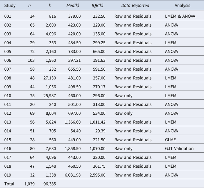
Note. n = number of participants per study. k = number of RTs per study. Med(k) = median RT length per study (raw data, 150 ms to 10,000ms). IQR(k) = Interquartile range of median RT length per study (ms). LMEM = Linear mixed effects model. GLME = generalized mixed effects model.
The re-analysis required the creation of a new, subdataset for each combination of outlier treatments, which consisted of the raw data, four transformations, nine sets of SD boundaries, winsorizing, and trimming (see Data transformations and Data cleaning sections below). This resulted in 95 subdatasets for each of the 19 useable datasets that were shared. The subdatasets for the first two re-analyzed studies, which equated to 190 subdatasets, were created manually using Microsoft Excel (Version 16.0.11929.20298). The subdatasets for the remaining 17 studies were generated using R (R Core Team, 2018). The manually produced subdatasets acted as checks to ensure that there were no errors with the R code for the generated subdatasets. In total, 1,805 subdatasets were created for re-analysis.
The first stage in creating the 95 subdatasets for each shared dataset consisted of removing extreme, time-based outliers from the raw dataset. Although time-based boundaries varied across studies, this variable was held constant at 150 ms for the lower boundary and 10,000 ms for the upper boundary. This decision was made in order to concentrate on the effects and interactions between data transformations and SD-based boundaries, which were the most common outlier treatments found in the synthesis of L2 SPR research (see Results section). The lower time-based boundary was theoretically driven by MEG research, where findings have suggested around 150 ms as a lower boundary for lexical identification (Hsu et al., Reference Hsu, Lee and Marantz2011). The upper boundary of 10,000 ms was selected as this was the highest boundary used for single word presentation across the 104 synthesized studies. Using such a large upper boundary guaranteed that outliers would be included, which was important because the aim of the current study was to investigate outlier treatments both individually and in concert. All RTs falling outside of the 150 to 10,000 ms boundary were removed from the initial raw dataset before any transformations or other outlier treatments were performed. The 95 subdatasets required for the re-analysis of each of the 19 shared datasets comprised of combinations of the following data transformations and data cleaning methods.
Data transformations
Each dataset from the 19 shared studies was initially transformed using (a) base 10 logarithmic transformation, (b) e logarithmic transformation, (c) Baayen's (Reference Baayen2008) inverse transformation (-1000/x), and (d) a square root transformation, resulting in five base datasets, including the original raw, untransformed set. Although the square root transformation was not implemented in any of the synthesized L2 SPR studies, it was included here, because it is one of the three Box-Cox procedure transformations. Some SPR studies involved centered RTs, or, in one case, RT z-scores for analysis, while a number of studies transformed RTs to residual RTs. These transformations were not implemented for re-analysis, because they are utilized for reasons other than outlier control.
Data cleaning
The five base datasets were subjected to a number of data cleaning methods involving SD-based boundaries. First, SDs for each participant or group were calculated, and a new dataset was created for each of the selected boundaries, -1.5 to 1.5, -2 to 2, -2.5 to 2.5, and -3 to 3, which represented the full range of boundaries used in the synthesized studies. To achieve as accurate a re-analysis as possible, the decision to use participant or group mean for determining the SDs for the boundaries followed the decision made by the original authors. Because reaction time distributions are positively skewed, asymmetrical boundaries holding the lower values were also investigated. Asymmetrical boundaries with a lower negative boundary were utilized, because they treat the tail end of the distribution more leniently, thus including true data points that would otherwise be eliminated. Such boundaries have also been shown to control for Type I errors and eliminate the effects of skewness (Keselman, Wilcox, Othman, & Fradette, Reference Keselman, Wilcox, Othman and Fradette2002). The asymmetric boundaries consisted of -1.5 to 2, -1.5 to 2.5, -1.5 to 3, -2 to 2.5, and -2 to 3, resulting in a total of nine different boundary combinations and, therefore, nine new datasets. Each of these datasets was subjected to both winsorizing and trimming, resulting in 18 new datasets for each of the five base datasets from the 19 studies. These SD-based data cleaning techniques were implemented on the untransformed set and the four transformed sets, resulting in 95 subdatasets per original shared dataset (see Figure 1), and a grand total of 1,805 subdatasets for analysis.

Figure 1. Composition of 95 subdatasets created for each of the 19 shared, raw datasets.
Statistics recorded
All subdatasets were re-analyzed with the same form of modeling as in the original study, which, in most cases, involved either factorial or repeated-measures ANOVA, or linear mixed-effects models (LMEMs). One set of SPR results was analyzed using a generalized linear mixed-effects (GLME) model, while another set was used to investigate the construct validity of GJTs (see Table 1). In this case, only the data removed and distribution statistics for the RTs, not the residual statistics, were recorded. For the studies involving ANOVA, re-analysis was conducted using R. For the studies involving LMEMs, re-analysis was conducted using the R package lme4 (Bates, Maechler, Bolker, & Walker, Reference Bates, Maechler, Bolker and Walker2015). If even one subdataset resulted in a singular fit, the model was simplified until a model could be successfully fit to all 95 subdatasets. This usually involved removing random slopes from the model one at a time, leaving critical slopes intact and avoiding random intercepts-only models where possible (Barr, Levy, Scheepers, & Tily, Reference Barr, Levy, Scheepers and Tily2013). In total, seven statistics were recorded from the re-analyses for further analysis. All of the results from the re-analyses and the R code used to produce them will be made available on the IRIS digital repository of instruments and materials for research into second languages (Marsden, Mackey, & Plonsky, Reference Marsden, Mackey, Plonsky, Mackey and Marsden2016).
Distribution statistics
The assumption of a normal, Gaussian distribution is perhaps the most well-known assumption of parametric testing, yet it goes unaddressed in the majority of L2 research (Al-Hoorie & Vitta, Reference Al-Hoorie and Vitta2019; Plonsky, Reference Plonsky2013). Outliers in the upper tail of an RT distribution can influence the shape of the distribution, making it inappropriate for numerous analyses. For ANOVA, the assumption of normality refers to the distribution of the dependent variable within each group, although ANOVA has been shown to be somewhat robust against skewed data (Glass, Peckham, & Sanders, Reference Glass, Peckham and Sanders1972). For regression methods utilizing continuous variables, including ANOVA, normally distributed residuals are a mathematical requirement (Baayen, Reference Baayen2008) and improve inferences made back to the population from which the sample was drawn (Pek, Wong, & Wong, Reference Pek, Wong and Wong2017; Williams, Grajales, & Kurkiewiwicz, Reference Williams, Grajales and Kurkiewicz2013). However, analyses are generally improved if all of the variables are also normally distributed (Tabachnick & Fidell, Reference Tabachnick and Fidell2013). In the present study, normality was assessed for (a) the ungrouped RTs for all subdatasets, and (b) the residuals for all subdatasets but three (see Table 1). Analysis of ungrouped data enabled the ANOVA- and LMEM-based data to be more easily compared.
In order to assess the distribution of the RTs and residuals under each treatment and detect outliers, skewness and kurtosis z-scores were calculated. First, skewness and kurtosis statistics were obtained through R using the psych package (Revelle, Reference Revelle2019). Next, the standard error (SE) of the skewness and kurtosis were generated from the n size using R code based upon the algorithms found in the SPSS manual (Seltman, Reference Seltmann.d.). The skewness and kurtosis statistics were then divided by their respective SEs to produce z-scores for the RT distributions in all 1,805 subdatasets. However, for the one study that investigated GJT construct validity, the two studies that could not be accurately re-analyzed, and the inverse transformation data for the study that utilized GLME, residual z-scores could not be recorded, meaning only 1,501 subdatasets contained residual skewness and kurtosis z-scores for further analysis. A threshold of 3.29 (p < .001) was used as a gauge of normality, whereby skewness and kurtosis values below -3.29 and above 3.29 are considered significantly different from zero (Tabachnick & Fidell, Reference Tabachnick and Fidell2013). Histograms were also consulted to assess normality.
In total, four distribution statistics were calculated for the majority of the 1,805 subdatasets consisting of skewness and kurtosis z-scores for the RTs, and skewness and kurtosis z-scores for the residuals. The effect of each of the 95 treatments on each of the four statistics was assessed individually using descriptive statistics and boxplots. If an outlier treatment displayed a strong effect on the z-scores, it could be considered as being either beneficial or detrimental for achieving a normal distribution.
Data Affected
For each of the 1,805 subdatasets, the percentage of data points excluded or altered by the data cleaning methods were recorded. This resulted in three values, representing the lower and upper tails of the distributions along with the combined total.
Data Analysis
Once the re-analysis was completed, a preliminary investigation of the data revealed some critical information that resulted in a number of subdatasets being removed from further analysis. First, although the log-e and log-10 transformation results produced different RT values, the statistics produced by the re-analyses for the two transformations were identical. For the final analyses, the subdatasets representing the log 10 results were thus discarded, and the log e results were used to represent log transformations. Second, boxplots revealed no significant difference between trimming and winsorizing with regard to any of the outcome statistics recorded (see Figure 2). Although the trimming condition produced negligibly superior results in terms of normalizing RT and residual distributions, the winsorized results were used in the subsequent analyses because winsorizing keeps potentially legitimate observations in a dataset, whereas trimming blindly removes them (Baayen, Reference Baayen2008). Third, subdatasets utilizing asymmetric boundaries in conjunction with an inverse transformation were removed, because this type of transformation resulted in both positive and negative skew. With negatively skewed data, using the asymmetrical boundaries resulted in leniency on the negative side of the distribution, which contradicted the reason for using such boundaries. Finally, inverse transformation results were removed for the study that utilized a GLME model, because lme4 was unable to process negative values for this type of analysis. Once all of these datasets were culled, 665 subdatasets remained for analysis.

Figure 2. Boxplots comparing the effects of trimmed and winsorized data on distribution statistics.
After these changes were made, the statistics listed above were analyzed using descriptive statistics, histograms, and boxplots. Because a number of the variables and distributions were nonnormal, medians and IQRs were reported as measures of central tendency and dispersion. Cohen's dav effect sizes, which are appropriate for within-group comparisons (Lakens, Reference Lakens2013), were calculated to determine the magnitude of a treatment's effect in comparison with the raw data and other treatments. Cohen's dav utilizes averaged SD values as a denominator; therefore, effect sizes were only calculated for distributions with skewness and kurtosis z-scores between -3.29 and 3.29 (see Supplementary Materials D, Tables 2–5). Effect sizes were interpreted according to Plonsky and Oswald's (Reference Plonsky and Oswald2014) within-group guidelines, whereby 0.60, 1.00, and 1.40 represent generally small, medium, and large effects in L2 research. However, caution should be adhered to when using such guidelines for RT data, because d values in psychology tend to be somewhat smaller (Brysbaert, Reference Brysbaert2019).
Results
Phase I: Synthesis of Outlier Treatment
Assessments of normality
As mentioned above, normally distributed data and residuals are important for the statistical methods utilized by SPR researchers. However, merely 18 (17.31%) of the sample studies analyzed mentioned this assumption. Of the 18 L2 SPR studies that did so, only six (5.77%) verified that the assumption was met. Five (4.81%) studies reported that the data were not normally distributed and used nonparametric statistics. A further four (3.85%) studies used logarithmic transformations to reduce skew. Only five (4.81%) studies detailed assumption statistics, with four (3.85%) reporting Kolmogorov-Smirnov Ds and one (0.96%) reporting a Shapiro-Wilk W, although these low numbers might be a relic of such tests being considered unreliable, especially with large samples (Field, Reference Field2018). Surprisingly, only three (2.88%) studies specifically mentioned the use of plots to assess normality, and only one (0.96%) specifically mentioned checking the residuals for normality.
Statistical analyses
Despite the vast majority of L2 SPR studies lacking reference to normality assumptions, all but two studies (98.08%) implemented statistical analyses that required normally distributed data or residuals. In total, 26 different parametric and nonparametric statistical analyses were conducted across the 104 studies. In 74 (71.15%) studies, RTs were analyzed with ANOVA, making it the most frequently used analysis. Factorial ANOVAs were employed in 42 (40.38%) studies, 37 (35.58%) analyzed both persons (F1) and items (F2), 33 (31.73%) specifically referred to repeated measures (even though F1 and F2 ANOVA incorporate repeated-measures), 15 (14.42%) used one-way ANOVA, and one (0.96%) study implemented multivariate ANOVA (MANOVA). Covariates were included in six (5.77%) studies, with five (4.81%) involving analysis of covariance (ANCOVA) and one (0.96%) involving multivariate ANCOVA (MANCOVA). The second most common analysis was LMEM, which was incorporated in 25 (24.04%) of the sample studies, the first of which was published relatively recently in 2011. Two studies (1.92%) utilized generalized linear mixed-effects models (GLMMs), and one (0.96%) utilized a logistic LMEM, all of which were published in 2019, suggesting that analyses involving data from L2 SPR are beginning to move toward mixed effects models.
Data transformations
Across the 104 studies that constituted the sample, RTs were subjected to four types of transformation. The most frequent two were the log (16.35%) and residual RT transformations (14.42%). Two (1.92%) studies standardized the RT data through z-score transformations, and another two (1.92%) involved log transformations performed in concert with centering. Only one (0.96%) study utilized an inverse transformation. The decision to utilize this transformation was a result of the only time that the Box-Cox procedure was implemented across the sample studies.
Data cleaning
Before focusing on the methods specifically implemented to control outliers, it is worth noting that 16 (15.38%) of the analyzed studies failed to address outliers at all. Of the 88 studies that addressed the issue, approaches to data cleaning included decisions regarding (a) the implementation of time-based and/or SD-based RT boundaries, (b) whether to use group-based, participant-based, or overall means when selecting SD-based boundary values, and (c) whether to eliminate or winsorize outliers.
Either time- or SD-based boundaries for outlier detection were employed by 84 (80.77%) of the sample studies. Time-based boundaries were implemented in 54 (51.92%) studies, with 12 (11.54%) using only lower boundaries, 15 (14.42%) using only upper boundaries, and 27 (25.96%) using both. For SPRs utilizing a word-by-word presentation, the median lower and upper time-based boundaries were 150 ms (IQR = 100) and 2,000 ms (IQR = 2,000), respectively. For SPR tasks utilizing a presentation type above the word level, including chunk-by-chunk, phrase-by-phrase, clause-by-clause, or sentence-by-sentence, the median lower and upper boundaries were 200 ms (IQR = 100) and 4,500 ms (IQR = 3,000).
Symmetrical, SD-based boundaries were utilized in 65 (62.50%) studies, with a median of 2.5 SDs (IQR = 1) in word-by-word presentations and two SDs (IQR = 0.5) for presentations larger than word level. The most popular choice was the -2 to 2 SD boundary, which was utilized in 29 (44.62%) of the 65 studies, followed by -2.5 to 2.5 SDs (30.77%), -3 to 3 SDs (23.08%), and -1.5 to 1.5 (1.54%). None of the studies in the sample incorporated asymmetrical SD-based boundaries. SPR researchers utilizing SD-based boundaries also faced a decision regarding which mean to base the SD upon. Of the 65 studies that incorporated SD-boundaries, participant or item mean was selected in 29 (27.88%) studies, 26 authors (25.00%) chose the group mean, just three (2.88%) chose the grand mean, and the selected mean was not specified in seven (6.73%) studies. Of the 17 studies utilizing log transformations, over half (58.82%) used the transformation in conjunction with SD-based boundaries.
The final decision facing SPR researchers concerned the choice of trimming or winsorizing. Of the 84 studies that implemented outlier detection boundaries, 64 (75.29%) trimmed the data, 12 (14.12%) winsorized the data, five (5.88%) used both, and eight (9.41%) replaced the boundary values with a mean. When winsorizing, all but two studies utilized SDs. Williams, Möbius, and Kim (Reference Williams, Möbius and Kim2001) winsorized outlying data with the participants’ next highest RT in that condition and position, and Jegerski (Reference Jegerski2018) winsorized with the upper time-based boundary (4000ms).
Phase II: Re-analysis of L2 SPR Studies
The following section contains the results of re-analyzed data from 19 published studies concerning the effect of outlier treatments on four distribution statistics. For space reasons, the results focus on the log and inverse transformations, which were the most successful, although the square root results are included in figures and tables for readers to make comparisons. In Figures 3a and 3c, which represent the RT skew and RT kurtosis respectively, each one of the 665 subdatasets that resulted from the re-analysis is represented as an observation. Figures 3b and 3d, which represent the residual skew and kurtosis, contain observations for each of the 555 subdatasets from which residuals were calculated. The boxplots are organized by transformation, with the nine SD boundaries and the raw, untreated datasets for each of the 19 studies nested within each transformation. On each of the boxplots, the two sets of dotted lines represent the 3.29 and -3.29 thresholds of a normal distribution. Observations falling between these two boundaries represent subdatasets with normally distributed RTs or residuals. The boxplots reveal that, for the majority of subdatasets in which no transformation was applied, the skewness and kurtosis z-scores of the RT and residual distributions were over 3.29, indicating that the subdatasets were inappropriate for parametric statistics. One residual observation and five RT observations with kurtosis z-scores greater than 60 were cropped for ease of interpretation (see Supplementary Materials D, Table 1 for comprehensive descriptive statistics). All of the outlying observations in Figure 3 represented unwinsorized subdatasets.

Figure 3. Boxplots illustrating the effect of data transformations on (a) RT skewness z-scores, (b) residual skewness z-scores, (c) RT kurtosis z-scores, and (d) residual kurtosis z-scores.
Once transformed, the majority of the z-scores for all three transformations across all four distribution statistics were within the critical boundary of -3.29 to 3.29. For the RT skewness (Figure 3a), log-transformation resulted in the most acceptable z-scores (median = 1.53, IQR = 1.30), followed by the inverse transformation (median = -1.80, IQR = 1.55). For the residual skewness (Figure 3b), the majority of the log-transformed (median = 1.30, IQR = 2.27) and inverse-transformed (median = 0.77, IQR = 1.27) subdatasets displayed acceptable z-scores. For the RT kurtosis z-scores (Figure 3c), the boxes representing the log-transformed (median = 0.37, IQR = 1.39) and the inverse-transformed RT distributions (median = 0.77, IQR = 1.45) were safely inside the 3.29 boundary. For the residual kurtosis (Figure 3d), the log-transformed (median = 0.87, IQR = 2.01), inverse-transformed (median = 0.90, IQR = 1.26) z-scores were slightly higher than those for the RT distributions, but were still overwhelmingly acceptable for parametric statistics. To summarize, prior to transformation, the vast majority of the RT and residual distributions were inappropriate for parametric statistics despite most subdatasets having been treated with SD boundary-based winsorizing. Once transformed, the vast majority of the distributions became acceptable. Because the SD boundary treatments were nested within the transformations, the next stage of the analysis focused on the effects of outlier treatments on RT and residual distributions at the SD boundary level.
For each of the four distribution statistics, boxplots were analyzed for the nine winsorized SD boundary treatments by transformation. Over 97% of the skewness and kurtosis z-scores were under 3.29 when analyzed by SD boundary (see Supplementary Materials D, Tables 2–5), therefore Cohen's dav effect sizes could be calculated for comparisons. For RT distributions, when neither transformation nor SD boundary treatment was utilized (median = 9.55, IQR = 5.66), the z-scores for skewness were almost always above the 3.29 boundary (see Figure 4a). The boxplots in Figure 4a also revealed that, for at least 75% of the untransformed subdatasets in each of the SD boundary treatments, the skewness z-scores were above 3.29 and, therefore, unsuitable for parametric analysis. This implies that regardless of the SD boundary utilized, the majority of winsorized RT distributions in the untransformed subdatasets were still too skewed to meet the assumption of normality. Figure 4b shows that once log-transformed, the RT distribution skewness in the majority of the SD boundary treatments became acceptable for parametric analysis. The Cohen's dav effect sizes comparing the nine winsorized SD boundary treatments on untransformed data with unwinsorized (i.e., no SD boundary implemented), log-transformed data ranged from 1.22 to 1.89, with all but one over 1.50, indicating a large effect (see Table 2). This implies that log-transforming data without winsorizing outliers had a stronger effect on the RT skewness z-scores than winsorizing untransformed data with any of the SD boundaries. Although the effect sizes are not reported here for space reasons, Figure 4b shows that implementing SD boundaries alongside log transformation reduced the skew even further. Such a reduction, however, comes at the cost of winsorizing potentially legitimate data. A weaker, but still substantial, effect was also found for the unwinsorized, inverse-transformed data, with effect sizes ranging from negligible, dav = 0.27, to medium, dav =0.82. However, these results should be taken with caution, because the mean of the inverse-transformed data, M = -3.26, SD = 4.66, was influenced by an outlier, z = -20.91 (see Figure 4c).

Figure 4. Boxplots illustrating the effect of SD boundary-based winsorizing on RT skewness z-scores by (a) untransformed, (b) log-transformed, (c) inverse-transformed, and (d) square root-transformed data. Note. “None” refers to unwinsorized data.
Table 2. The Effect of Unwinsorized, Transformed Data on RT Skewness (z) Compared with Untransformed, Winsorized Data (Cohen's dav)

Note. For the inverse transformed data, skewness z-score = -5.31, kurtosis z-score = 7.90.
Table 3. The Effect of Unwinsorized, Transformed Data on RT Kurtosis (z) Compared with Untransformed, Winsorized Data (Cohen's dav)

Table 4. The Effect of Unwinsorized, Transformed Data on Residual Skewness (z) Compared with Untransformed, Winsorized Data (Cohen's dav)

Table 5. The Effect of Unwinsorized, Transformed Data on Residual Kurtosis (z) Compared with Untransformed, Winsorized Data (Cohen's dav)

Figure 5 displays the results of the re-analyses on the kurtosis z-scores of the RT distributions across the 665 subdatasets. Outliers were cropped from Figure 5a (z = 116.56) and Figure 5c (z = 89.78) for ease of interpretation. Both outliers were included in the analysis, because they were legitimate results and did not disrupt the log- and square root-transformed data to the same extent. As with the RT skewness results, Figure 5a shows that the distributions of the nontransformed, unwinsorized subdatasets (median = 27.87, IQR = 32.79) were almost all inappropriate for parametric statistics. The same figure also suggests that, apart from the -1.5 to 1.5 SD boundary, winsorizing the data did not adequately attend to the kurtosis problem in the majority of the subdatasets. In comparison, the log transformation of unwinsorized data addressed the kurtosis, with effect sizes ranging from negligible for within-group L2 data, dav = 0.40, to large, dav = 1.54 (see Table 3). The distribution of the unwinsorized, inverse-transformed data suffered from large skewness, z = 6.79, and kurtosis, z = 11.74, rendering them inappropriate for calculating Cohen's dav. Comparison of central tendency measures (median = 1.53, IQR = 3.20, compared with M = 7.26, SD = 20.22) emphasized this inappropriacy. However, the results are included in Table 3 as a demonstration of how a single outlier can contaminate results. The boxplots representing the unwinsorized log- and inverse-transformed data in Figures 5b and 5c, which are based on the median, suggest that 75% of the results for both transformations are within the -3.29 to 3.29 boundary. Whereas the mean-based effect sizes of the log-transformed data were generally large, the effect sizes for the inverse data were all negligible, ranging from -0.33 to 0.19. However, when the outlier was removed, the central tendency measures, M = 2.68, SD = 3.18, and the effect size range, 0.20 to 1.36, changed dramatically (see Table 3). The single outlier disguised the substantial effect of the inverse transformation over the SD boundary treatments on untransformed data.

Figure 5. Boxplots illustrating the effect of SD boundary-based winsorizing on RT kurtosis z-scores by (a) untransformed, (b) log-transformed, (c) inverse-transformed, and (d) square root-transformed data. Note. “None” refers to unwinsorized data.
Figure 6 illustrates the results of the re-analyses of the z-scores for the skewness of the 555 subdatasets from which residuals were recorded. Figure 6a shows that when untransformed data were subjected to certain SD boundary treatments, for example, -1.5 to 1.5, -2 to 2, or -1.5 to 2, the skewness of the residuals for around half of the subdatasets became acceptable for parametric statistics. However, these boundaries are the three most costly in terms of data affected by trimming and winsorizing (see Figure 7). When compared with the untransformed SD boundary treatments, log transformation of unwinsorized data had less of an effect on the residual skew than on the RT skew, with values ranging from small, dav = 0.46, to fairly large, but medium in the context of L2 research, dav = 1.21 (see Table 4). In terms of the effect on residual skew, the inverse-transformation on unwinsorized data had a stronger effect than the log transformation, ranging from medium, dav = 1.00, to large, dav = 1.60. However, the inverse transformation was again more prone to extreme outliers (see Figure 6c).

Figure 6. Boxplots illustrating the effect of SD boundary-based winsorizing on residual skewness z-scores by (a) untransformed, (b) log-transformed, (c) inverse-transformed, and (d) square root-transformed data. Note. “None” refers to unwinsorized data.

Figure 7. Boxplots illustrating the percentage of data affected by each SD boundary treatment.
Finally, Figure 8 illustrates how the pattern of the kurtosis z-scores of the residual results was analogous to the RT results. The untransformed, unwinsorized results contained an extreme outlier, z = 140.15, which was more than twice the size of the second largest value. This outlier was cropped from Figure 8a for ease of interpretation. In comparison with the untransformed SD boundary treatments, log transformation of unwinsorized data had a marginally smaller effect on the residual kurtosis than the RT kurtosis, with values ranging from negligible, dav = 0.31, to considerable, but medium in the context of L2 research, dav = 1.30 (see Table 5). These effect sizes were, however, stronger than the equivalents for the inverse-transformation, which ranged from 0.20 to 1.18. Figure 8c shows that the inverse-transformed data was once again prone to outliers.

Figure 8. Boxplots illustrating the effect of SD boundary-based winsorizing on residual kurtosis z-scores by (a) untransformed, (b) log-transformed, (c) inverse-transformed, and (d) square root-transformed data. Note. “None” refers to unwinsorized data.
To summarize, logarithmic transformation had the greatest effect on the RT and residual distributions in terms of both skewness and kurtosis. When compared with untransformed results in conjunction with any of the SD boundary treatments, logarithmic transformation of unwinsorized data displayed larger effects on the distribution statistics, without the need to blindly exclude or adjust the value of outliers. Inverse transformation results were almost as effective but were more susceptible to the effect of extreme outliers. Unsurprisingly, the boxplots show that skewness and kurtosis can be reduced further by combining transformation with winsorizing. However, winsorizing and trimming were unnecessary in the majority of cases, because log-transformations were successful at reducing skewness and kurtosis to acceptable levels for parametric analysis, thus preserving potentially legitimate data points. Although the analyses were performed on winsorized data, the results are generalizable to trimmed data, because there is no substantial difference between the distributions produced by the two different data cleaning methods (see Figure 2).
Discussion
Phase I: Synthesis of Outlier Treatment
The first research question pertained to general outlier treatment in L2 studies involving SPR. The most notable finding of the synthesis of L2 SPR tasks was confirmation of the lack of uniformity regarding outlier treatment. When time-based boundaries were implemented, not only were different times utilized across the sample of studies, but discordancy existed between the use of an upper boundary, lower boundary, or both. Of the 65 studies that utilized SD boundaries, a -2 to 2 SD boundary was most common (44.62%), followed by -2.5 to 2.5 (30.77%), -3 to 3 (23.08%), and -1.5 to 1.5 (1.54%). However, a discrepancy existed between studies regarding which mean to utilize when calculating SDs, whether it be the participant or item mean (27.88%), group mean (25.00%), or grand mean (2.88%), while a number of researchers (6.73%) failed to specify which mean was used. As stated by Marsden et al. (Reference Marsden, Thompson and Plonsky2018), such opaqueness coupled with the discordancy between outlier treatments hinders comparability of individual study results.
Slightly more consistency was displayed in terms of transformation and data cleaning methods. In terms of transforming data to specifically account for skewness, the log transformation was by far the most common (16.35%), followed by the inverse transformation (0.96%). However, these amounts seem low considering the results above implying that transformations address outliers more effectively than SD boundaries. In over half of the studies involving log transformation, SD boundaries were also used, which introduced more inconsistency between studies. Also, despite log transformations being the most frequently implemented, only one study mentioned the base value used for the transformation. For data cleaning, trimming (75.29%) was far more frequent than winsorizing (5.88%) across the 85 studies that implemented SD boundaries, despite the potential of trimming to eliminate legitimate data.
Another notable finding of the research synthesis was the lack of reference to normality assumptions. Merely 17.31% of the sample mentioned normality assumptions. However, this result is comparable to 17.00% found in a survey of SLA study quality (Plonsky, Reference Plonsky2013), 16.00% in L2 written corrective feedback (Liu & Brown, Reference Liu and Brown2015), 15.53% in regression studies (Plonsky & Ghanbar, Reference Plonsky and Ghanbar2018), and 16.82% reported for five focal statistical procedures when a stringent standard is adhered to (Hu & Plonsky, Reference Hu and Plonsky2019). These figures become particularly worrisome considering the fact that 98.08% of the synthesized studies implemented parametric statistics that require normally distributed residuals to make dependable inferences back to the population (Pek et al., Reference Pek, Wong and Wong2017; Williams et al., Reference Williams, Grajales and Kurkiewicz2013). Of these parametric statistics, ANOVA (71.15%) proved to be the most common. However, despite the first use of LMEMs in L2 SPR research being in 2011, 24.02% of the sample utilized this method, suggesting that, as with L1 psycholinguistic research, LMEMs are on their way to becoming a new standard in L2 psycholinguistic research. If LMEMs do replace ANOVA as the method of choice for L2 psycholinguistics experiments, it does not mean that the normality distribution can be dismissed. LMEMs are a member of the generalized linear model (GLM) family of regression models, and, as such, assume that data are normally distributed (Baayen, Reference Baayen2008; Barr et al., Reference Barr, Levy, Scheepers and Tily2013; Cunnings, Reference Cunnings2012; Linck & Cunnings, Reference Linck and Cunnings2015).
Phase II: Re-analysis of L2 SPR Studies
In Phase II of the current study, methods for treating outliers and normalizing skewed RT distributions were investigated in order to address the second research question: How do the various outlier treatments utilized in L2 SPR research affect RT data? A number of treatments were considered, consisting of data cleaning, transformations, and SD boundaries. The two data cleaning methods investigated, trimming and winsorizing, were found to have almost identical effects on the distribution of both the RTs and the residuals (see Figure 2). Boxplots showed that winsorizing was slightly less efficient than trimming at reducing skewness and kurtosis and was also marginally more prone to outliers. However, these differences were negligible. Winsorizing was utilized for analysis in the current study and is recommended because it keeps potentially legitimate observations that would be removed by trimming.
Log e, inverse, and square root transformations were implemented on the datasets, and their effects were compared with each other and also with nontransformed data. Log 10 transformation data were excluded from the analysis, because they produced identical results to the log e transformation in terms of the statistics reported above. Log e results were preferred in the current study and are recommended for consistency in future studies for two reasons. First, log e coefficients can be interpreted as proportional differences in regression. A coefficient of 0.10 indicates an approximate 10% difference in y for every difference of 1 in x (Gelman & Hill, Reference Gelman and Hill2007). Second, log transformations with higher bases, such as 10, have a tendency to affect extreme values more dramatically than lower values (Osborne, Reference Osborne2002). Although neither of these reasons specifically relate to outliers in SPR tasks, if L2 researchers habitually use log e in place of log 10, it will make no difference in terms of the SPR task results but might be beneficial, if RTs are submitted to other forms of analysis not considered in the present study.
Of the three transformations applied here, log e consistently produced superior results in repairing RT and residual distributions in terms of both skewness and kurtosis. Although the inverse transformation was as effective for the majority of the subdatasets, it was also more prone to outliers and has been shown to lower statistical power (Schramm & Rouder, Reference Schramm and Rouder2019). Judging by the preference for log transformation displayed by researchers utilizing L2 SPR tasks, this finding might not be new. However, a minority of L2 SPR studies (16.35%) involved log transformations, and over half of those combined the transformation with SD-based trimming, perhaps unnecessarily. The results above also showed log transformation to be more effective than merely using any combination of SD boundary on untransformed data, and in the vast majority of cases also controlled kurtosis and skewness at both the RT and residual level, without recourse to the elimination or alteration of data. Of course, combining log transformations with SD boundaries reduced skewness and kurtosis further, but overlapping boxplots suggested that the difference was not significant, and, therefore, not worth the cost of losing potentially legitimate data.
Although log transformations successfully controlled skewness and kurtosis in the current study, transformations not only affect the structure of the data but also potentially affect the corresponding effect sizes (Pek et al., Reference Pek, Wong and Wong2017). The conversion from raw to log scores also entails a conversion from arithmetic means to geometric means, which are invariably less than arithmetic means and change the construct and hypothesis being tested (Field, Reference Field2018). For instance, most cognitive theories were developed and validated using untransformed RTs. Therefore, utilizing transformed RTs to test a hypothesis is tantamount to utilizing a different dependent variable to the one on which the theoretical underpinnings were based (Lo & Andrews, Reference Lo and Andrews2015). Alternatively, conversion to geometric mean might be considered beneficial for RT data. As mentioned previously, RT data are generally skewed, with outliers in the upper tail that influence the mean and SD of a distribution, which in turn affects the results of any mean-based statistical analysis, including the calculation of standardized mean difference effect sizes such as Cohen's d (see Table 3).
In a recent study, VanPatten and Smith (Reference VanPatten and Smith2019) commented on how the effects of trimming data at predetermined SD boundaries are unclear and that the “practice has come under increased scrutiny” (p. 411). The findings of this study, based on an investigation of nine different SD boundaries, suggested that deliberating over whether to use 2 or 2.5 SD boundaries (which accounted for little over 75% of boundary choices in L2 SPR research) and then trimming the data that falls outside is not the most effective method of handling outliers in L2 SPR research. In fact, the median z-scores for the distribution statistics investigated in this study fell outside of the 3.29 zone when symmetrical 2 or 2.5 SD boundaries were implemented on untransformed data (see Figures 4, 5, 6, and 8), rendering them inappropriate for parametric analysis. When combined with the paradox that SD boundaries are calculated from means containing the outliers that the SD boundaries are intended to combat, and the potential for SD boundaries to eliminate or alter legitimate data, it seems unadvisable to utilize SD boundaries on L2 SPR data. Logarithmically transforming data was much more successful in handling outliers and achieving normal distribution in terms of skewness and kurtosis at both the RT and residual level and did not require the exclusion of potentially legitimate data. Combining log transformations with SD boundaries also seems unwarranted because the transformation repaired the distribution in the vast majority of cases.
The final research questions asked whether one method of outlier treatment was particularly suited to L2 SPR research. Although a “one-cap-fits-all” solution to outlier treatment is unrealistic, the preceding investigation revealed patterns that informed the following recommendations. First, if the raw data are normally distributed at both the RT and residual level, as attested to by histograms, boxplots, and skewness and kurtosis z-scores, then there is no need for any outlier treatment. Second, if the data are nonnormally distributed, log transformation should be utilized, as it generally made the distributions acceptable for statistical analyses without recourse to elimination or alteration of potentially legitimate data points. Third, if the RT or residual skewness or kurtosis is still unacceptable after log transformation, it might be worthwhile to investigate the outlying data points at the tail end of the distribution individually to determine why they are different from the majority of the data, as opposed to blindly eliminating them. If a reason cannot be determined, then results should be reported both with and without outliers, along with justification of why data points were removed or winsorized (Aguinis et al, Reference Aguinis, Gottfredson and Joo2013; Aguinis & Joo, Reference Aguinis, Joo, Lance and Vandenberg2015; Baayen & Milin, Reference Baayen and Milin2010; Bakker & Wicherts, Reference Bakker and Wicherts2014; Kruskal, Reference Kruskal1960; Ratcliff, Reference Ratcliff1993; Simmons et al., Reference Simmons, Nelson and Simonsohn2011; Streiner, Reference Streiner2018). The presentation of both analyses enables readers to come to their own conclusions regarding a set of results and might help combat the practice of outlier removal with the sole aim of finding support for hypotheses (Cortina, Reference Cortina2002). However, caution should be exercised even if the results of an analysis are reported with and without outliers included as there is no way of determining which one of the analyses is the best representation of the target population (Orr et al., Reference Orr, Sackett and Dubois1991). Finally, if a researcher still believes that SD boundaries are required to identify which data points are outliers, winsorizing should be implemented as opposed to trimming, as winsorizing avoids the blind elimination of legitimate data and produces results that are quantitively equivalent to trimming (see Figure 2).
Future Research
These recommendations should be considered a starting point as further research is warranted to account for the discrepancy between studies with regard to time-based boundaries, and to investigate the viability of statistical methods that do not require data transformations. In the current study, an upper boundary of 10,000 ms was utilized, which was intentionally large in order to include outliers. The results of the research synthesis indicated that, for word-by-word presentations, the median upper boundary implemented by L2 SPR researchers was 2,000 ms. This seems fairly strict, especially if low- or mid-proficiency participants are involved. However, Table 1 shows that the median RT length for all but one of the studies was under 1,900 ms, which included studies presenting stimuli at the phrase level, therefore 2,000 ms might be reasonable. The outlying value in Table 1, median = 6,031.98, was from the only study that incorporated sentence-by-sentence presentation. The lower boundary of 150 ms was based on MEG research suggesting that somewhere between 100 ms to 200 ms is the minimum time required time for lexical identification (Hsu et al., Reference Hsu, Lee and Marantz2011). However, literature pertaining to minimum word recognition times is based upon L1 speakers; therefore, further research should be conducted with L2 learners to determine an empirically justifiable lower time boundary for L2 SPR/RT research. Further research is also warranted into statistical analyses that do not rely on a normal distribution. The current study illustrates the benefits of log transformations, but adds the caveat that such transformations potentially affect the structure of the data and the corresponding effect sizes. If RT distributions are inherently nonnormally distributed and require transformations to meet linearity assumptions, perhaps analyses that do not assume linear distributions, such as GLMEs, should be considered instead (see Baayen, Reference Baayen2008; Tamura, Fukuta, Nishimura, Harada, Hara, & Kato, Reference Tamura, Fukuta, Nishimura, Harada, Hara and Kato2019).
Beyond our proposed implications for the handling of outliers, we would also like to draw attention to the importance of data sharing. The present study would not have been possible without the willingness of individual researchers to locate and share their data with us, and we are immensely grateful for their assistance. At the same time, it is somewhat disheartening that such willingness seems to be more the exception than the rule. As applied linguistics continues to embrace open science practices such as open materials and study preregistration (see Gass, Loewen, & Plonsky, Reference Gass, Loewen and Plonskyin press; Marsden, Morgan-Short, Trofimovich, & Ellis, Reference Marsden, Morgan-Short, Trofimovich and Ellis2018; Marsden & Plonsky, Reference Marsden, Plonsky, Gudmestad and Edmonds2018), we hope that more researchers take steps toward transparency throughout their workflow. Doing so will not only allow for more robust findings in studies such as ours, but it will also allow for greater interpretability of and trust in empirical findings.
Limitations
The findings of the current study are not without limitations. First, although a great deal of praise is owed to the researchers who took the time to reply to our data request, and even more to those who were able to share their data, the final data set consisted of just 19 studies. This sample size severely reduced the number of statistical procedures that could be utilized in the data analysis and arguably affects the generalizability of the results. Second, the difference between the mean used is a variable that was not accounted for in this study. In certain datasets, SD boundaries were calculated from participant means, while in others, group means were utilized. Although it is possible that using a participant mean, when determining an SD boundary, might increase or reduce the normality of an RT distribution, when compared with a group mean, there is no theoretical reason or precedent set in the literature for believing that it would. Also, the findings of the current study led to our recommendation of avoiding SD boundaries, making the choice of which mean to use a moot point. Finally, it should be emphasized that the findings are specific to L2 SPR RTs only and are not intended to be used for other techniques that incorporate RTs, such as GJTs and lexical decision tasks, which require longer RTs of at least 300 ms (Jiang, Reference Jiang2012). We encourage others to consider undertaking a study similar to ours with data from those and other domains of L2 research.
Conclusion
In sum, 104 studies involving L2 SPR tasks were synthesized to investigate the treatment of outliers. The synthesis results revealed substantial inconsistency at nearly all decision points. In an attempt to find the outlier method most suited to L2 SPR research, a set of 19 datasets (N = 1,039) from published studies incorporating SPR results were acquired and re-analyzed using a number of common outlier treatments to establish their relative effectiveness for attending to outliers and normalizing SPR RT data.
The results of the re-analysis suggested that, in the vast majority of cases, natural logarithmic transformation of RT data circumvented the need for SD boundaries. When compared with untransformed, in conjunction with any of the SD boundary treatment, logarithmic transformation of unwinsorized data displayed larger effects on the distribution statistics without the need to blindly exclude or alter the value of outliers. Results also indicated that the choice of SD boundary had little to no influence on the distribution of the data. Additionally, there was no quantitative difference found between trimming and winsorizing data. Together, these results suggest that L2 SPR researchers should log transform RT data when the dependent variable and/or residuals are nonnormally distributed. If the skewness and kurtosis of these distributions remain problematic after log transformation, then outliers should be investigated individually to determine their cause. If researchers still wish to employ SD-based boundaries to remove outliers, we recommend winsorizing as opposed to trimming in order to avoid the elimination of legitimate data.
Empirically supported norms for methodological decisions, such as how to handle outliers, are important for producing comparable studies. Although these recommendations are merely the first step toward such norms, we believe that they are an important step. We also believe that this study serves as an example of how Open Science practices, such as data sharing and re-analysis, can be beneficial for researchers in applied linguistics.
Supplementary material
The supplementary material for this article can be found at https://doi.org/10.1017/S0267190520000057


