3.1. Skymask generation

In the offline stage, the building boundaries are projected on the skyplot, termed ‘skymask’ in this paper. If the satellite elevation is lower than the building boundary elevation (under the same azimuth angle), the signal is assumed to be the NLOS signal blocked by buildings.

The skymask of each location is generated with the 3D city model offline, as shown in Algorithm 1. Thus, the skymask can be initially stored in the device. Based on the 3D building model or in storage perspective, a specific area is selected and divided into grid points to construct the skymask table; the grid point separation is 2 m to generate the skymask. Here, an assumption is made that the candidate is always on the ground (mean sea level). Therefore, in this study, the height of the skymask position is given by the mean sea level datum provided by the Hong Kong Lands Department (Survey and Mapping Office, 1995). Figure 2 is an example of the generated skymask and storage format. The azimuth is in one-degree resolution; the elevation is in 0·1-degree resolution; and the building height is in one-metre resolution. The azimuth angle starts from the north direction, rotating in a clockwise direction; the elevation angle starts from the horizon as zero degrees.

Algorithm 1 Skymask generation on a specific location

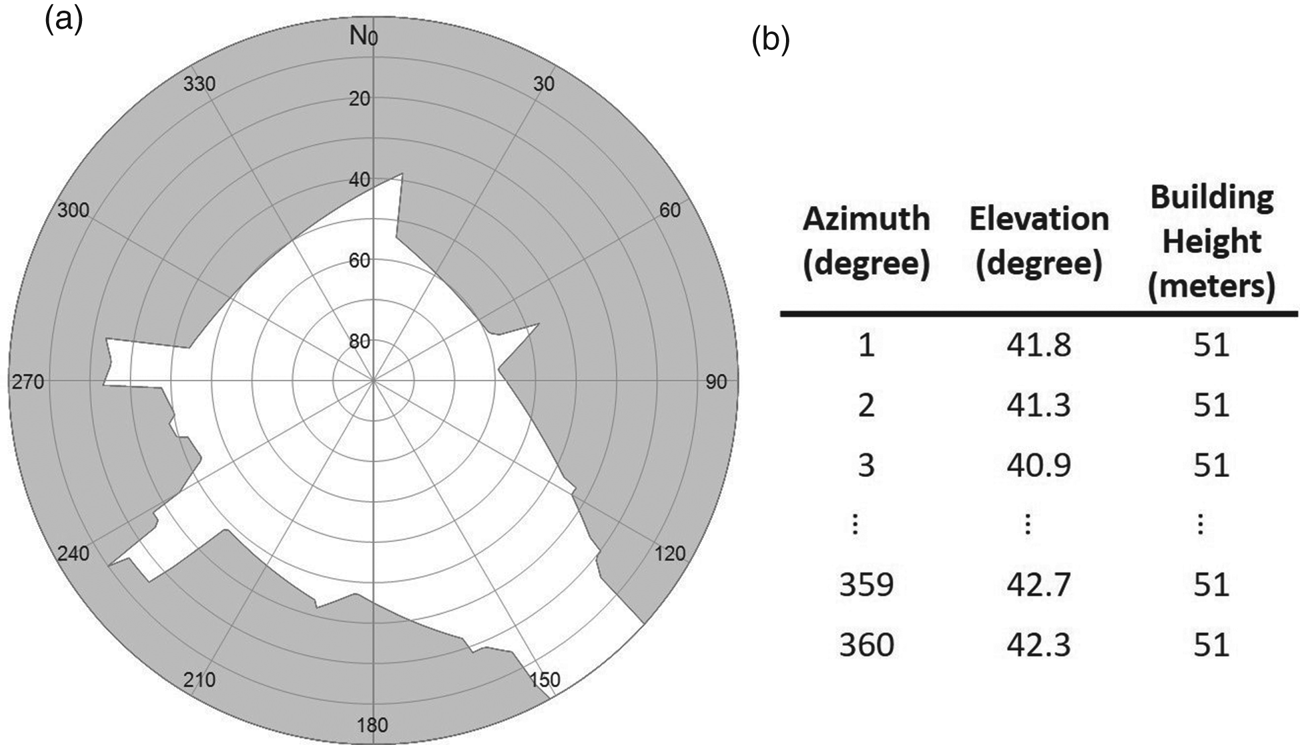
Figure 2. Example of skymask (a) and skymask array (b).

Each location will first be classified as to whether it is inside the building. For the ‘outside building’ location, a matrix of 360-by-2 will be used to store the skymask for single location, first column store the maximum elevation angle of the building edge for the corresponding azimuth angle; second column store the building height on the corresponding azimuth angle, as shown in Figure 2, for later use to find the valid reflecting point. For the ‘inside building’ location, a flag will be given to represent this is a building.

This offline generation perspective is especially important for a low-cost device with limited computational power, as it is nearly impossible for such devices to generate the skymask every time in both time consumption and power management aspects. This step is similar to the process proposed in Wang et al. (Reference Wang, Groves and Ziebart2012), but the enhanced skymask includes the building height information associated with each azimuth angle for NLOS correction usage.

3.2. Detection of reflecting points on skymask

In the real-time positioning, theoretically, an initial position is first given by single point positioning at each epoch to distribute positioning candidates around. To provide a more sophisticated initial solution, the National Marine Electronics Association (NMEA) position provided by the receiver will be used in this paper. A grid of searching area with 40 m radius and 2 m separation between adjacent candidates will be constructed. Since the skymask information is pre-computed based on grids, distributing the candidate in the same grids makes it feasible to load the corresponding skymask information directly and avoids applying interpolation. If the candidate is distributed inside the building, it will not calculate its likelihood. The satellites are then projected onto the skyplot of each candidate based on their position estimated using ephemeris data, as well as loading the corresponding skymask. As a result, the satellites can be classified into LOS and NLOS from the candidate skymask. Figure 3 shows the flow to determine the reflecting point from the skymask for the NLOS satellite.

Figure 3. Flowchart of reflecting point detection.

With the skymask information of the candidate, we should determine the AARP value on each surrounding building surface, as shown in Algorithm 2. The geometric meaning is the parallel direction of the building surface where the reflection occurs. The AARP value, φ, is the building surface's parallel direction in azimuth angle with respect to north in the clockwise direction, as shown in Figure 5. Note that determination of the AARP value can be processed in the offline stage by the server or in the online stage by the receiver. The advantage of processing by the server when generating the skymask is that it can obtain the AARP value directly from the 3D building model. The advantage of online calculation is that it can reduce the storage required on the receiver, as the AARP value on each grid needs to be stored with the skymask if calculated offline.

Algorithm 2 AARP-based possible reflected signal incoming direction prediction

Unlike the 3D building model used in the ray-tracing 3DMA GNSS (Hsu et al., Reference Hsu, Hu and Kamijo2016a), surrounding buildings are mixed together in the skymask and are not separable. Thus, it is important to identify the individual building surface since each surface may have a different AARP. The building boundary on the skymask can be illustrated as a curve with respect to the elevation and azimuth, as in Figure 4. As shown in Figure 5, the corresponding AARP needs to be identified to estimate the valid reflecting point for a different building.

Figure 4. Plot of skymask (Figure 5(b)) in elevation-azimuth format and determined feature points. Red, green and blue points are feature points; purple lines represent valid surface; black lines are invalid surface; grey shadowed area is the blue surface in Figure 5.

Figure 5. Actual position (a) and polar position projected on skymask (b). Red arrow is the AARP for the blue surface that causes reflection and φ is the axis direction angle; orange line is the direct path blocked by building; purple line is the reflecting path. Orange and purple points on the skymask represent the signal incoming azimuth and elevation angle of the direct and reflected path, respectively.

Two features from the skymask curve are extracted to determine the corresponding AARP of the potential reflection surface. The first feature is the sudden changing point, corresponding to the building boundary points with over two degrees of elevation angle difference between two adjacent points. The curve between two sudden changing points indicates the transition to different buildings, which is invalid for signal reflection. The skymask curve with small change (less than two degrees) represents a valid surface for signal reflection. The second feature is the local minima or maxima within the valid curve. The feature points could be representing the different visible surface from the candidate.

This is followed by identifying the valid surface and its orientation from the skymask. As mentioned above, the feature points represent the building corners. Therefore, the azimuth angles between two consecutive feature points will be considered as one surface. In two exceptional cases, if two adjacent azimuth angles (e.g., az and az+1) are sudden change points, it means this change to another building and surface should exist, and it will not be considered as a surface. Another such situation is the elevation of zero degrees, as there is assumed to be no valid reflector on the ground.

After obtaining the feature points including sudden change points, local minima and local maxima, the AARP on each azimuth angle is computed by two adjacent feature points. The possible reflected signal incoming direction ψ_az regarding the building surface on different azimuth direction az can then be computed with step 20 in Algorithm 2. Therefore, for a specific satellite i, the corresponding signal reflecting point azimuth can be obtained by matching the known satellite azimuth azⁱ with the predicted possible reflected signal incoming direction, as follows

(1)$${\rm az}_{{\rm Refl}}^i =\mathop{\arg\,\min}\limits_{{\rm az}\in \{ {1^{\circ}, 2^{\circ}, \ldots , 360^{\circ}}\}} ( {\psi_{{\rm az}} -{\rm az}^i} ) $$

Note that if no existing ψ_az fulfils $\vert {\psi_{{\rm az}} -{\rm az}^{i}}\vert \lt1^{\circ}$ for a satellite at a candidate, no valid reflecting signal can be found for this satellite on this candidate position.

The AARP determination algorithm aims to provide a more accurate possible reflection surface determination based on skymask; the results can be illustrated using Figures 6 and 7. In the Figure 6 environment, the orientation of the red surface is different from other surfaces. The actual AARP of surrounding surfaces are expressed with purple arrows in Figure 6. The purple arrows in Figure 7 show the AARP determined by our proposed algorithm. From the results, the algorithm can identify the correct AARP of the surrounding surface, as well as some small visible surface from the location's skymask.

Figure 6. Complex environment (a) with multiple axis directions and corresponding skymask (b). Blue arrow is the along-street direction; purple arrows are the surrounding visible surface AARP; the red curve in (a) represents the red surface in (b).

Figure 7. Demonstration of the result by the proposed AARP algorithm. Green point is the ground truth location in Figure 6; black solid line is the building contour; colour points are the location used on the skymask, the colour represents the elevation angle; purple arrows represent the AARP vector determined by propose algorithm.

As indicated in Hsu (Reference Hsu2018), NLOS delay can be modelled with elevation angle and lateral distance from the receiver to the reflector. Therefore, after determining the AARP and predicting the incoming signal direction with the candidate's skymask, we can detect the reflecting point and output actual position.

Before detecting the reflecting point from the AARP found in the above step, we need to know the angular relationship between the receiver, satellite position and AARP. As shown in Figure 8(a), the satellite elevation at the receiver is the same as at the reflecting point provided that the reflecting surface is vertical, since the satellite is far away from the reflecting point and receiver. With the law of reflection, the incident angle is equal to the reflection angle which is the elevation angle of the reflecting point, as θ_elev. On the other hand, on the view above from the receiver, as shown in Figure 8(b), an AARP is defined as parallel to the building surface that reflects the NLOS signal. Since the satellite is far away from the receiver and the reflecting point, the incident reflected signal (from satellite to reflected plane) is parallel to the direct signal, the angle between reflected plane and incident reflected signal (or 90°-incident angle) equals the azimuth angle between the AARP and the direct signal, as γ_azi. Due to pure reflection behaviour, the incident angle is equal to the reflection angle, which is also equal to the azimuth angle between the reflecting point and the AARP (which is parallel to the reflecting surface). Therefore, the location of the reflecting point can be estimated by the satellite elevation and azimuth angles with respect to the receiver in the skymask. As Figure 5 shows, based on the preceding relationship, the valid reflecting point (purple point) of the GNSS signal on the building surface can be determined symmetrically to the satellite position (orange point) on the skymask with respect to the AARP.

Figure 8. (a) side view to demonstrate the angular relationship between the direct and reflected signal on elevation; (b) top view to demonstrate the azimuth angle relationship. Green and blue line represent reflect and direct path respectively; red arrow is the AARP of reflection causing surface (red framed building).

Finally, the horizontal distance from candidate to building height on the corresponding reflecting point's azimuth can be resolved by building height and elevation angle to the building edge. By further combining with the azimuth and elevation angle of the reflecting point, the actual position of the reflecting point can be obtained by converting from local coordinates to Earth-Centered, Earth-Fixed (ECEF) using the standard coordinate transformation matrix.

As well as the reflection delay of i-th satellite on n-th candidate, $\varepsilon _{n}^{{\rm refl}( i) }$, is calculated by the total geometric distance of the reflect path (1. Satellite to reflecting point, $D_{{\rm Refl}}^{{\rm SV}}$; and 2. Reflecting point to the receiver, $D_{{\rm RCV}}^{{\rm Refl}} ) $ then subtract the geometric distance of direct LOS path, $D_{{\rm RCV}}^{{\rm SV}}$.

(2)$$\varepsilon _n^{{\rm refl}(i)} =D_{{\rm Refl}}^{{\rm SV}} +D_{{\rm RCV}}^{{\rm Ref}l} -D_{{\rm RCV}}^{{\rm SV}}$$

3.3. Simulated range calculation

To evaluate the likelihood of the position candidates, the difference between pseudorange measurement ρ̃ and simulated range ρ̂ on each position candidate is required. The simulated range $\hat{\rho}_{n}^{i}$ between the i-th satellite and the n-th position candidate can be calculated by the sum of the geometric distance $R_{n}^{i} $, correction for satellite clock and orbit offset, $c\delta t_{i}^{{\rm sv}}$, ionosphere errors (using the Klobuchar model (Klobuchar, Reference Klobuchar1987)), I ⁱ, and troposphere errors, T ⁱ and reflection delay distance, $\varepsilon _{n}^{{\rm refl}( i) }$ found in Section 3.2 if applicable, as follows,

(3)$$\hat{\rho}_n^i=R_n^i c\delta t_i^{{\rm sv}}+I^i+T^i\varepsilon _n^{{\rm refl}(i)}$$

To eliminate the receiver clock offset, a reference satellite will be selected. All measurements and simulated ranges are differenced once to obtain the single difference of the ranges on each candidate. The reference satellite r(i) is selected by the LOS satellite with the highest elevation angle for each constellation on each candidate. Note that inter-constellation timing bias could be obtained from the broadcast navigation message. In that case, we can consider all the measurements are from the same constellation.

(4)$$D_n^i =|(\tilde{\rho}_n^i-\tilde{\rho}_n^{r(i)})-(\hat{\rho}_n^i-\hat{\rho}_i^{r(i)})|$$

The similarity of the candidate αⁿ is calculated by averaging the single difference range $D_{n}^{i}$. Table 1 shows the rule of signal type classification; the measurements can be classified into LOS and NLOS by the machine learning suggested by Sun et al. (Reference Sun, Hsu, Xue, Zhang and Ochieng2018) and the prediction of the enhanced skymask. This classification applies to each candidate and measurement individually. If and only if the satellite visibility is consistent between the proposed method and signal strength classification, the corresponding measurement will be included in the candidate score calculation; the N _sim denotes the number of valid range differences. Note that if the reference satellite is the only satellite that agrees on signal type, this candidate will not be scored and will be labelled as invalid.

(5)$$\alpha^n=N_{{\rm sim}}^{-1} \times \sum_i^{N_{{\rm sim}}}{D_n^i }$$

The average of range difference will then rescale between 0 to 1 to become the score of the candidates. The smaller the value of the average of the range differences, the higher the score; in other words, the simulated range is a better match with the measurement.

(6)$$\mbox{score}^n=\frac{\max ( \alpha ) -\alpha ^n}{\max ( \alpha ) -\min ( \alpha ) }$$

The final step is to determine the position solution of the skymask 3DMA algorithm. All the candidates' scores are then used to calculate the weighted average position. As a result, the positioning solution can be obtained and the positioning solution will apply the height information from the pre-computed skymask grid point information.

(7)$$x( t ) =\frac{\sum_n {( {\mbox{score}^n( t ) P^n( t ) } ) } }{\sum_n {\mbox{score}^n( t ) } }$$

4.1. Experiment setup

A commercial-grade GNSS receiver (u-blox EVK-M8T with u-blox ANN-MS patch antenna) was used to record raw measurements. The output rate of the receiver was set at 1 Hz. The constellations on single-frequency GPS and BeiDou satellite were enabled. The second static experiment also included measurements recorded by Xiaomi Mi 8. The results of the experiments were then post-processed, and the positioning results using the following algorithms were compared:

1. 1. WLS: weighted least square (Realini and Reguzzoni, Reference Realini and Reguzzoni2013)

2. 2. RT: ray-tracing based 3DMA GNSS (Hsu et al., Reference Hsu, Hu and Kamijo2016a)

3. 3. SKY: skymask based 3DMA GNSS, the method proposed in this paper

Both the ray-tracing algorithm and the proposed skymask based 3DMA GNSS consider only the single reflection, and provide correction only for reflection-found NLOS signals. The difference between the proposed method and the ray-tracing algorithm is that the former uses the skymask to obtain the NLOS correction. Therefore, we can evaluate the accuracy of the proposed method by comparison with ray-tracing.

The experiments were conducted in two urban areas of Hong Kong. The dynamic experiment and one static experiment (experiments 1 and 2) were conducted in Tsim Sha Tsui, (TST); and the second static experiment (experiment 3) was conducted in Tsuen Wan (TW), as shown in Figure 9. The referencing ground truth of each experiment is manually labelled based on Google Earth. The walking velocity of the dynamic experiment was assumed to be uniform, so ground truth is given by interpolating between starting point and destination with the total experiment time. The dynamic experiments took 69 s with about 70 m walking distance while the static experiments took 2 min (120 epochs). The experimental environment can be described as shown in Table 2. In terms of the proposed axis determination method, the environment of experiment 1 is relatively simple compared with that of experiment 3.

Figure 9. Experiment locations: (a) Tsim Sha Tsui (b) Tsuen Wan, Hong Kong.

Table 2. Experiment environment.

Note that the ratio of building height to street width is calculated by building height/street width, which means that the value is higher when the street is narrower with taller buildings surrounding it and the experiment environment is more challenging for positioning. The ‘AARP determination error at ground truth’ was evaluated by comparing the AARP derived from the proposed method in Section 3.2 with the AARP obtained from the 3D building model in Google Earth, and further demonstrated by mean value and standard deviation of the difference between all azimuth angles.

4.2. NLOS reflection detection and correction accuracy

The ground truth from the two static experiments is used here to execute the skymask and ray-tracing based 3DMA GNSS methods to see whether the proposed method provides a consistent reflection delay distance compared with ray-tracing prediction results.Tables 3 and 4 include the total signal, which is labelled as NLOS where reflection was found or not by both methods. Totals of 1,371 and 1,345 signals were found in the TST and TW static experiments (experiments 2 and 3), respectively.

Table 3. LOS/NLOS signal labelling in experiment 2 (static).

Table 4. LOS/NLOS signal labelling in experiment 3 (static).

From the above results, the rate of correct signal classification was about 87% in TST and 70% in TW. However, some signals were mislabelled, as the ray-tracing classified them as LOS while the skymask 3DMA classified them as NLOS with no reflection found, as the direct paths of these signals were too close to buildings. This shows a potential problem of the skymask method in handling the uncertainty of the building edge model, where some of the signals may miss detection if they are near the building edge. As a result, there is a difference in classifying the signal type. Another main issue was when the ray-tracing method labelled signals as NLOS with no reflection found and the skymask method labelled them as NLOS with reflection found. The main reason is that the ray-tracing assumes a perfect single reflection, where two parts of the reflected signal path ((1) satellite to reflecting point; and (2) reflecting point to the receiver) are not blocked by any buildings. However, the skymask method did not verify that the path from satellite to reflecting point was free of blockage, so it resulted in misidentification of the reflection found.

Furthermore, to evaluate the range level correction, we used the ground truth of the experiments, and performed 3DMA GNSS to extract the NLOS range correction and compare it with the double difference. The NLOS correction should be similar to the double difference residual if it is accurate enough. Using the satellite BeiDou B11 in TST (experiment 2) and BeiDou B7 in TW (experiment 3) to analyse further the NLOS correction accuracy in range level, we compared NLOS correction between:

1. 1. NLOS delay by double differencing technique (D.D. estimated delay) (Xu et al., Reference Xu, Jia, Luo and Hsu2019)

2. 2. Proposed skymask 3DMA

3. 3. Ray-tracing

The reflection correction of the proposed method can achieve a similar result to the ray-tracing one, the mean of the correction difference between skymask 3DMA and ray-tracing for BeiDou B11 in TST was 2·02 m with standard deviation of 0·01 m, and the average difference between skymask 3DMA and double difference was 3·75 m with standard deviation of 2·35 m. The mean difference between skymask 3DMA and ray-tracing of BeiDou B7 in TW was 1·84 m with standard deviation of 0·00 m; the average difference between skymask 3DMA and the double difference is 1·58 m with standard deviation of 1·46 m. Other corrections provided by skymask 3DMA were also comparable with the ray-tracing results, the average being within about 10 m difference.

Table 5 summarises the means and standard deviations of the NLOS delay from the proposed skymask 3DMA method and ray-tracing method for two satellites among all the satellites as examples. The performance is further compared with the NLOS delay estimated by the double difference technique using the reference station data and user's true location. It can be observed that the proposed skymask 3DMA can provide a similar accuracy in range level correction compared with the ray-tracing method and actual measurement.

Table 5. Summary of NLOS reflection delay identified by three methods.

4.3. Positioning results

The dynamic experiment (experiment 1) was undertaken in TST, as shown in Figure 10 and Table 6. The u-blox receiver collected the raw measurements during walking along the designed path to simulate a pedestrian scenario.

Figure 10. Dynamic experiment results in Tsim Sha Tsui.

Table 6. Dynamic experiment results in TST.

The along-street direction of the dynamic experiment is 139 degrees and this angle is used to analyse the positioning error in the along-street and across-street directions. It can be observed that the overall performance of the proposed skymask 3DMA GNSS is over 10 m better than the WLS solution in mean error. The proposed skymask 3DMA GNSS has an extra error of about 1 m on the two-dimensional (2D) and along-street direction, while the across-street direction can achieve similar accuracy to the ray-tracing algorithm.

In experiment 2, data was collected by the u-blox and Xiaomi Mi 8 for a duration of 240 s. The positioning results and statistics are shown in Figure 11 and Table 7, respectively.

Figure 11. Static experiment results in Tsim Sha Tsui. (a) data recorded by u-blox; (b) data recorded by Xiaomi Mi 8.

Table 7. Static experiment results in TST by u-blox and Mi 8.

From the positioning results, the skymask 3DMA GNSS algorithm can achieve similar positioning results compared with the ray-tracing based 3DMA GNSS algorithm for the u-blox receiver. For the across-street direction, especially, the root mean square (RMS) error of skymask 3DMA is better than that of the ray-tracing algorithm. The Mi 8 positioning results were worse than the ray-tracing in 2D and along-street error, but the across-street obtained slightly better results than ray-tracing.

As shown in Figure 12, a static experiment took place in TW with u-blox only (experiment 3). The experimental environment is a dense urban area with streets just 10 m wide, and the building height-to-street width ratio is 2·29. Furthermore, the experiment was located at the intersection of two perpendicular streets. Therefore, the environment potentially has multiple axes. The positioning error statistics are shown in Table 8.

Figure 12. Static experiment results in Tsuen Wan.

Table 8. Static experiment results in TW.

In experiment 3, the skymask method could also achieve a similar accuracy compared with the ray-tracing method. The 2D error was about 12 m for the skymask method, 10 m and 6 m error on along- and across-street directions, respectively, while the ray-tracing 2D error was 8 m, with along- and across-street directional error as 6 m and 4 m, respectively.

4.4. Computational load

The post-processing of the experimental data was performed by an Intel 7th Generation Intel^® Core™ i7 Processor, with Matlab programming platform. The skymask 3DMA was found to be about 10 times faster than ray-tracing in single epoch positioning. Table 9 summarises the average processing time for post-processing for different positioning algorithms and the time reduction. The ‘Reduction on percentage’ is calculated by $((t_{{\rm RT}}-t_{{\rm SKY}})/t_{{\rm RT}}) \times 100{\rm \% }$ where t _RT and t _SKY are the average processing duration for one epoch for ray-tracing and skymask 3DMA, respectively. The ‘Difference of 2D RMS error’ is calculated by RMS_SKY − RMS_RT, where RMS_RT and RMS_SKY are RMS error of ray-tracing and skymask 3DMA respectively. A negative value here means extra positioning error was observed from the ray-tracing 3DMA GNSS.

Table 9. Average processing time for experimental data.