


1. Introduction
Over the past decades, coherent structures in wall-bounded turbulent flows ranging from low Reynolds number flat, smooth-wall boundary layers to the atmospheric boundary layer (ABL), have been the focus of numerous studies and have been recognized as being major contributors to the turbulent transfer of momentum, heat and mass (Marusic et al. Reference Marusic, McKeon, Monkewitz, Nagib, Smits and Sreenivasan2010b; Smits, McKeon & Marusic Reference Smits, McKeon and Marusic2011). Identified as organized motions that are persistent in time and space, various types of coherent structures with different origin, lifecycle, scales and characteristics have been evidenced, depending on the Reynolds number of the flow, the distance from the wall, the wall roughness, the presence of a pressure gradient or the stability regime of the flow if the ABL is considered. However, even if they share common features and that a consensus has emerged for smooth-wall-bounded flows such as pipe flows, channel flows or flat-plate boundary layers (Smits et al. Reference Smits, McKeon and Marusic2011), their interaction and the associated mechanisms remain unclear. On the basis of the recent advances achieved for smooth-wall-bounded flows, the main objective of the present contribution is to investigate the interaction between the lower-atmosphere and vegetation canopy flow, a configuration in which the presence of the canopy significantly changes the nature of the coherent structures in the near-wall region (Finnigan Reference Finnigan2000; Dupont & Brunet Reference Dupont and Brunet2009; Finnigan, Shaw & Patton Reference Finnigan, Shaw and Patton2009). In the following sections of the introduction, we first present the results from recent studies obtained in the smooth-wall configuration regarding the interaction between the near-wall turbulence and the larger scales of the flow. The characteristics of the coherent structures present both in the canopy region and in the ABL are then presented. The last part of the introduction details the objectives of the present contribution.
1.1. Scale interaction in boundary-layer flows
Because of their geometrical simplicity and their relevance to many fundamental and industrial or environmental problems, flat-plate boundary layers (FPBLs) have received a great deal of attention. A detailed description of their characteristics has been achieved, which can be found in recent reviews from the literature (Robinson Reference Robinson1991; Panton Reference Panton2001; Adrian Reference Adrian2007; Marusic et al. Reference Marusic, McKeon, Monkewitz, Nagib, Smits and Sreenivasan2010b; Smits et al. Reference Smits, McKeon and Marusic2011). The structure of turbulence in this type of flow is now understood to be characterized by coherent structures that can be classified by their size and which are: (i) the inner streaks related to the near-wall cycle and associated with (ii) packets of hairpin vortices (Adrian Reference Adrian2007) which constitute the large-scale motions (LSMs) and (iii) the very-large-scale motions (VLSMs). Both numerical and experimental studies have highlighted the influence of the latter on the near-wall turbulence and their contribution to the turbulent kinetic energy and Reynolds shear stress in different type of wall-bounded flows such as pipe flows (Monty et al. Reference Monty, Stewart, Williams and Chong2007), channel flows (del Alamo & Jimenez Reference del Alamo and Jimenez2003), laboratory boundary layers (Marusic & Hutchins Reference Marusic and Hutchins2008) and ABL over a hydrodynamically smooth surface (Guala, Metzger & McKeon Reference Guala, Metzger and McKeon2011; Hutchins et al. Reference Hutchins, Chauhan, Marusic, Monty and Klewicki2012). Common features of the VLSMs found in wall-bounded flows are that (i) they consist of elongated low- and high-speed regions (Hutchins & Marusic Reference Hutchins and Marusic2007), the length of which scales with outer-length variable  $\delta$ (the boundary layer thickness) and can reach several times
  $\delta$ (Guala et al. Reference Guala, Metzger and McKeon2011), (ii) they populate the log and outer layer, they are animated by a meandering motion in the horizontal plane (Hutchins & Marusic Reference Hutchins and Marusic2007) and (iii) interact with near-wall turbulence. The mechanism by which near-wall turbulence and these large-scale structures interact has been found to consist of both a linear superimposition of the large scales onto the near-wall turbulence and a nonlinear interaction which has been identified as being similar to an amplitude modulation (AM) of the near-wall fluctuations by the larger scales of the flow. This latter mechanism has received renewed attention since the work of Bandyopadhyay & Hussain (Reference Bandyopadhyay and Hussain1984) and has been clearly characterized and quantified, mainly for the longitudinal velocity component (Mathis, Hutchins & Marusic Reference Mathis, Hutchins and Marusic2009; Chung & McKeon Reference Chung and McKeon2010; Hutchins & Marusic Reference Hutchins and Marusic2010; Hutchins et al. Reference Hutchins, Monty, Ganapathisubramani, Ng and Marusic2011; Jacobi & McKeon Reference Jacobi and McKeon2013). All the proposed methods to analyse the AM effect are based on low-pass filtering the instantaneous fluctuating velocity signal
  $u$ into a large-scale component
  $u^L$ and a small-scale component
  $u^S = u- u^L$ and quantifying the AM strength using the normalized correlation between
  $u^L$ and the low-pass-filtered envelope of
  $u^S$ (known as the AM correlation coefficient, see § 3.4 and Jacobi & McKeon Reference Jacobi and McKeon2013). When applied to single-point measurements, the utility of this scale-decomposition method relies on a clear spectral separation between the near-wall energetic scales and those in the outer region of the flow. A two-point version of this approach has also been proposed and showed similar results (Mathis et al. Reference Mathis, Hutchins and Marusic2009; Bernardini & Pirozzoli Reference Bernardini and Pirozzoli2011). Both Mathis et al. (Reference Mathis, Hutchins, Marusic and Sreenivasan2011b) and Schlatter & Örlü (Reference Schlatter and Örlü2010) noted the strong resemblance between the skewness of the signal
  $u$ and the AM correlation coefficient. Using a phase-scrambled synthetic signal respecting the statistics of the velocity signal
  $u$ up to the third-order moment, Schlatter & Örlü (Reference Schlatter and Örlü2010) showed that the similarity between the velocity skewness and the AM correlation coefficient was a direct consequence of the intrinsic properties of
  $u$. Mathis et al. (Reference Mathis, Hutchins, Marusic and Sreenivasan2011b) further noted that the AM correlation coefficient was also quantitatively similar to the contribution to the skewness of the cross-term
  $\langle u^L (u^S)^2 \rangle$. Chung & McKeon (Reference Chung and McKeon2010) and Jacobi & McKeon (Reference Jacobi and McKeon2013) showed that the correlation between the large scales and the envelope of the small scales can be interpreted as a measure of the phase lag between the different scale motions. Cui & Jacobi (Reference Cui and Jacobi2021) used a bispectral and corresponding biphase analysis of channel flow direct numerical simulation to demonstrate that the phase of the small-scale motions leads the LSMs due to delays that arise from nonlinear triadic interactions. Jacobi & McKeon (Reference Jacobi and McKeon2013) and Talluru et al. (Reference Talluru, Baidya, Hutchins and Marusic2014) demonstrated that all small-scale velocity components in the near-wall region of a boundary layer experience a similar AM influence from the large scales. Harun et al. (Reference Harun, Monty, Mathis and Marusic2013) showed that the AM of small scales by the LSMs also exists in boundary layers subjected to the presence of both adverse or favourable pressure gradients and that its intensity increases with increasing pressure gradient from favourable to adverse.
Investigation of the AM of the near-wall turbulence by the larger scales of the boundary layer has been extended to rough-wall configurations. Using hot-wire measurements conducted in a wind tunnel, Squire et al. (Reference Squire, Morill-Winter, Hutchins, Schultz, Klewicki and Marusic2016) showed its existence in sand-roughened-wall boundary layers. It was also confirmed by Pathikonda & Christensen (Reference Pathikonda and Christensen2017) in the flow over complex roughness with a wide range of topographical scales arranged in an irregular manner. Existence of the same type of AM mechanism has also been demonstrated in turbulent boundary layers developing over two-dimensional obstacles (Talluru et al. Reference Talluru, Baidya, Hutchins and Marusic2014; Nadeem et al. Reference Nadeem, Lee, Lee and Sung2015; Blackman, Perret & Savory Reference Blackman, Perret and Savory2017) and cube arrays (Anderson Reference Anderson2016; Blackman & Perret Reference Blackman and Perret2016; Basley, Perret & Mathis Reference Basley, Perret and Mathis2018). In all these configurations, the basic nature of the interaction mechanism remains the same as in smooth-wall configurations. The strength of AM was, however, found to be stronger than in FPBLs, mainly because of the modification of the near-wall turbulence by the presence of the large roughness elements. Blackman, Perret & Calmet (Reference Blackman, Perret and Calmet2018) extended these coefficient correlation based investigations by interrogating a scale-decomposed budget of turbulent kinetic energy in a boundary layer developing over staggered cubes, demonstrating that AM is linked to an instantaneous exchange of energy between the large-scale momentum regions and the small scales close to the roughness. Within this context, Salesky & Anderson (Reference Salesky and Anderson2018) recently investigated the influence of buoyancy effect on the large scales – near-wall turbulence interaction using large-eddy simulation (LES) of the ABL. AM of the small-scale turbulence was found to exist for all atmospheric stability cases, the wall-normal LSMs playing an increasing role with increasing convective effects.
An important consequence of having observed and quantified the relationship between the near-wall turbulence and the larger scales of the flow is that Marusic, Mathis & Hutchins (Reference Marusic, Mathis and Hutchins2010a) and Mathis, Hutchins & Marusic (Reference Mathis, Hutchins and Marusic2011a) were able to formulate a simple predictive model of the longitudinal velocity fluctuations in the near-wall region using a so-called universal small-scale signal modulated by a measured large-scale velocity signature and superimposed onto a large-scale component. Their modelling approach has recently been tested by Blackman, Perret & Mathis (Reference Blackman, Perret and Mathis2019) in the turbulent boundary layer developing over cube arrays. These authors showed that the near-wall modulated signal is no longer universal but dependent on the roughness array arrangement. They nevertheless confirmed that, for a given wall configuration, the model's parameters were Reynolds number independent, at least in the Reynolds number range they investigated.
Analysis of AM showed the influence of the large scales onto the near-wall smaller scales from a global point of view. At the same time, recent studies have investigated this scale-interaction mechanism through the derivation of the scale-by-scale transport equation of the turbulent kinetic energy and Reynolds shear stress; an approach that provides detailed information on the interscale and/or spatial transport of the turbulent kinetic energy (TKE) and the Reynolds stresses at different scales. Given the numerous spatial gradients involved in computing the different transport terms, such studies are mainly based on data from numerical simulations. Mizuno (Reference Mizuno2016) recently analysed the energy transport in channel flows based on the evaluation of the spectral energy budget equation. He showed the existence in the near-wall region of downward energy fluxes at large scales, responsible for the Reynolds number dependence of both the velocity fluctuations and the dissipation rate, consistent with the observations of the influence of the large scales onto the near-wall scales based on AM analysis. Mizuno (Reference Mizuno2016) also stressed the importance of the role played by spatial transport, even if its intensity is weak compared with that of production or dissipation. In particular, because budget analysis only provides the ability to estimate average energy transport, instantaneous transport from small to large scales might be counterbalanced by other events and therefore remains hidden. Reference Lee and MoserLee & Moser's (Reference Lee and Moser2019) detailed spectral analysis of the energy balance in a channel flow confirmed that the VLSMs, which dominate and drive the energy transfers in the outer region, actually transfer energy to the wall region which result in modulation of the near-wall cycle and the Reynolds number dependence of the velocity variances in this region. Lee & Moser (Reference Lee and Moser2019) also revealed energy transport away from the wall. Kawata & Alfredsson (Reference Kawata and Alfredsson2018) investigated the possible existence of a feedback mechanism from the small to the large scales by extending the above scale-by-scale analysis of energy transport to the Reynolds shear stress in a low Reynolds number plane Couette flow. While they confirmed the net supply of energy from the large to the small scales, they demonstrated that the Reynolds shear stress is transferred from small to large scales throughout the channel. This might support production of TKE at large scales and therefore constitute the feedback loop of the small scale–large scale interaction mechanism. To the authors’ knowledge, apart from that by Blackman et al. (Reference Blackman, Perret and Calmet2018) who conducted a two-scale decomposed budget, the analysis of Kamruzzaman et al. (Reference Kamruzzaman, Djenidi, Antonia and Talluru2015) represents a rare investigation of AM in rough-wall configurations. These authors recently performed a scale-by-scale budget for the second-order structure function of the streamwise velocity component in a turbulent boundary layer over a rod-roughened wall and showed the influence of the large-scale inhomogeneities in the flow on intermediate scales over which the transfer of energy is important.
1.2. Coherent structures in vegetation canopy flow
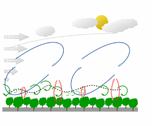
The importance of coherent structures has also been recognized in more complex wall-bounded flows and numerous studies have been devoted to the structure of boundary-layer flows developing over rough walls, at laboratory scales (see Jimenez (Reference Jimenez2004) for a review) or in neutrally stratified atmospheric flows over urban or vegetation canopies (Dupont & Brunet Reference Dupont and Brunet2009; Finnigan et al. Reference Finnigan, Shaw and Patton2009; Inagaki & Kanda Reference Inagaki and Kanda2010; Takimoto et al. Reference Takimoto, Sato, Barlow, Moriwaki, Inagaki and Kanda2011), which demonstrate some of the similarities and differences between flows over smooth and rough walls. The most complete description of the average turbulence structure in the near-canopy region has been obtained for vegetation canopies because of: (i) their relatively simpler geometrical configuration when compared with urban canopies, (ii) the homogeneity of the vegetation at scales relevant for the flow and (iii) the development of the mixing-layer analogy (whose validity for urban flows has yet to be shown) (Raupach, Finnigan & Brunet Reference Raupach, Finnigan and Brunet1996; Finnigan Reference Finnigan2000). Canopy eddies have been the subject of intensive research conducted based on outdoor field measurements, wind tunnel and water tunnel experiments (Gao, Shaw & Paw Reference Gao, Shaw and Paw1989; Collineau & Brunet Reference Collineau and Brunet1993; Ghisalberti & Nepf Reference Ghisalberti and Nepf2002; Poggi et al. Reference Poggi, Porporato, Ridolfi, Albertson and Katul2004; Patton et al. Reference Patton2011; Perret & Ruiz Reference Perret and Ruiz2013; Zeeman et al. Reference Zeeman, Eugster, Christoph and Thomas2013) and numerical simulations (Su et al. Reference Su, Shaw, Paw U, Moeng and Sullivan1998; Fitzmaurice et al. Reference Fitzmaurice, Shaw, Paw U and Patton2004; Watanabe Reference Watanabe2004; Dupont & Brunet Reference Dupont and Brunet2009; Finnigan et al. Reference Finnigan, Shaw and Patton2009; Watanabe Reference Watanabe2009; Bailey & Stoll Reference Bailey and Stoll2016). The important role that coherent structures play in turbulence production, being major contributors to time-averaged turbulence statistics, and also in the transfer of momentum and scalars is now well admitted. Based on the mixing-layer analogy (Raupach et al. Reference Raupach, Finnigan and Brunet1996), a conceptual model for their generation and evolution has been proposed, in which canopy eddies originate from the Kelvin–Helmholtz instabilities induced by the existence of an inflection point in the mean velocity profile at canopy top, that roll into spanwise vortices; these spanwise rolls further evolve into complex three-dimensional structures (Finnigan & Brunet Reference Finnigan and Brunet1995). The major contributors to the momentum transport were found to be strong sweeps and weaker ejections embedded in elongated region of low or high momentum, of elliptical shape (Shaw et al. Reference Shaw, Brunet, Finnigan and Raupach1995). Raupach et al. (Reference Raupach, Finnigan and Brunet1996) hypothesized that large-scale structures bringing high-momentum fluid down to canopy top likely enhance canopy-top shear locally which serves to trigger the Kelvin–Helmholtz instability at canopy top. Finnigan & Shaw (Reference Finnigan and Shaw2000) completed this description with the presence of a single head-down hairpin, found by applying empirical orthogonal decomposition to wind tunnel data. Performing a conditional analysis using local maxima of static pressure at canopy top as a trigger from LES data, Finnigan et al. (Reference Finnigan, Shaw and Patton2009) were able to improve this model and show the existence a pair of head-down and head-up hairpin vortices responsible for the induction of sweeps and ejections, respectively (figure 1). This pressure-based compositing strategy also evidenced the presence of sharp scalar microfronts that can be expected to exist at the boundary between the sweeps and ejections. It has been found that these ejections and sweeps, the latter being more numerous than the former close to the canopy and conversely away from the wall, leave a strong imprint in the skewness of both the longitudinal and vertical velocity components (Finnigan Reference Finnigan2000). From the analogy between canopy flow and a plane mixing layer (Raupach et al. Reference Raupach, Finnigan and Brunet1996), the relevant length scale of coherent motion in and above vegetation canopies is thought to be the shear length scale  $L_s = \langle u \rangle /( \partial \langle u \rangle /\partial z )$, evaluated at the height of the inflection point in the mean longitudinal velocity profile. Typical length scales of coherent motions within vegetation canopies have also been quantified using integral time or length scales derived from temporal or two-point spatial correlations, respectively. Combining the integral time scale with a convection velocity corresponding to the velocity of the canopy-scale structures in the canopy-top region (estimated here as the local mean velocity) in order to use Taylor's hypothesis, Brunet, Finnigan & Raupach (Reference Brunet, Finnigan and Raupach1994) found that the corresponding longitudinal integral length scales
  $L_u$ and
  $L_w$ of the streamwise and vertical velocity components, respectively, were much larger than the size of the individual canopy elements and increased with height within and just above the canopy. At the top of the canopy,
  $L_u /h \simeq 1$ and
  $L_w /h \simeq 3$, where
  $h$ is the height of the canopy. Using two-point correlation coefficients, Shaw et al. (Reference Shaw, Brunet, Finnigan and Raupach1995) directly computed integral length scales and showed that they varied much more slowly and were larger (
 $L_u /h \simeq 2.75$ and
  $L_u /h \simeq 0.5$ at the top of the canopy) than when computed using temporal information combined with Taylor's hypothesis. This discrepancy was explained by Raupach et al. (Reference Raupach, Finnigan and Brunet1996) as being a direct consequence of the poor estimate of the convection velocity
  $u_c$ of canopy eddies by the local longitudinal velocity. Using two-point data, a new estimate of the convection velocity was computed and found to be close to
  $u_c = 1.8 \langle u(h) \rangle$, showing that local mean velocity is not a good estimation for the convection velocity of the canopy-scale structures and that the latter are connected to the outer larger-scale flow (Shaw et al. Reference Shaw, Brunet, Finnigan and Raupach1995; Raupach et al. Reference Raupach, Finnigan and Brunet1996). The mean longitudinal spacing of canopy eddies
  $\varLambda _x$ has been characterized by using the location
  $f_{max}$ of the maximum in the pre-multiplied temporal energy spectrum of the vertical component
  $w$ with the improved estimation of the convection velocity proposed by Raupach et al. (Reference Raupach, Finnigan and Brunet1996). It is therefore defined as
  $\varLambda _x / h = f_{max}u_c / h$ (Raupach et al. Reference Raupach, Finnigan and Brunet1996). Observation of this parameter in various vegetation canopy flows revealed that in near-neutral stability regime a linear relationship between
  $\varLambda _x$ and
  $L_s$ exists, namely
  $\varLambda _x/ L_s = 8.1$ (Raupach et al. Reference Raupach, Finnigan and Brunet1996). Departure from the near-neutral stability regime has been found to influence the typical length scales of the canopy eddies, the shear length scales
  $L_s$ decreasing when the stability condition changes from a free-convection to a stable regime, the streamwise spacing
  $\varLambda _x / L_s$ or
  $\varLambda _x / h$ showing a non-monotonic evolution with the stability regime while being maximum in near-neutral conditions (Brunet & Irvine Reference Brunet and Irvine2000; Dupont & Patton Reference Dupont and Patton2012; Patton et al. Reference Patton, Sullivan, Shaw, Finnigan and Weil2016).
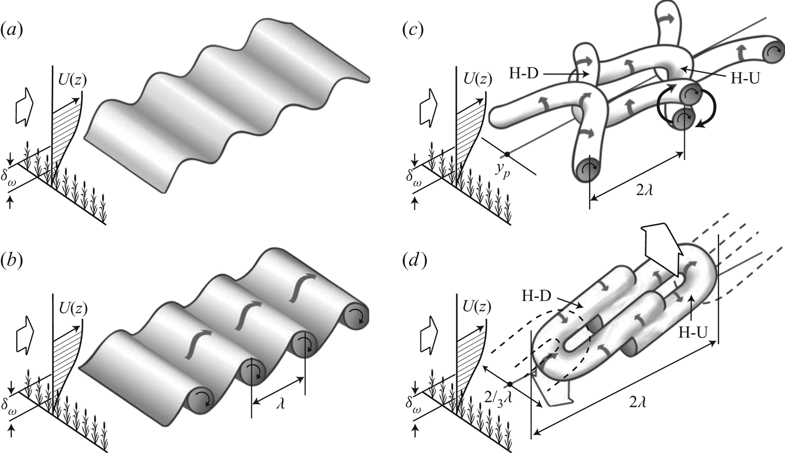
Figure 1. Schematic diagram of the dual-hairpin eddy formation from Patton & Finnigan (Reference Patton and Finnigan2013) (adapted from Finnigan et al. Reference Finnigan, Shaw and Patton2009).
1.3. Large-scale coherent structures in the ABL
As noted by Raupach et al. (Reference Raupach, Finnigan and Brunet1996) and Watanabe (Reference Watanabe2004), the above-described canopy flow is always under the influence of the coherent eddies of the ABL, the scales of which are typically of the order of the boundary-layer depth. The detailed presentation of the characteristics of the coherent structures encountered in the ABL is beyond the scope of the present description. Only a brief overview of the coherent structures and their main features is therefore presented here in order to show that, whatever the stability regime of the ABL, vegetation canopy flows and near-surface turbulence in general are immersed in larger-scale motions and are likely to be influenced by it through similar mechanism as in FPBLs. In the case of neutrally stratified stability regime, for which wind shear is the primary mechanism producing turbulence, coherent structures in the ABL were found to share many similarities with those found in smooth-wall laboratory boundary-layer flows. Streaky structures consisting of elongated regions of low- or high-speed streamwise velocity were found in flows studied via numerical simulations (Deardorff Reference Deardorff1972; Moeng & Sullivan Reference Moeng and Sullivan1994; Lin et al. Reference Lin, McWilliams, Moeng and Sullivan1996a,Reference Lin, Moeng, Sullivan and McWilliamsb; Khanna & Brasseur Reference Khanna and Brasseur1998; Shah & Bou-Zeid Reference Shah and Bou-Zeid2014; Fang & Porté-Agel Reference Fang and Porté-Agel2015) and field campaigns (Drobinski et al. Reference Drobinski, Carlotti, Newsom, Banta, Foster and Redelsperger2004; Horiguchi et al. Reference Horiguchi, Hayashi, Hashiguchi, Ito and Ueda2010, Reference Horiguchi, Hayashi, Hashiguchi, Adachi and Onogi2012; Hutchins et al. Reference Hutchins, Chauhan, Marusic, Monty and Klewicki2012). The typical streamwise dimension of these structures is of the order of several hundreds of metres (Drobinski et al. Reference Drobinski, Carlotti, Newsom, Banta, Foster and Redelsperger2004). Lin et al. (Reference Lin, Moeng, Sullivan and McWilliams1996b) showed that the transverse spacing (normal to the surface-wind direction) of the streaks evolves linearly as a function of height above ground, in agreement with the measurements of Drobinski et al. (Reference Drobinski, Carlotti, Newsom, Banta, Foster and Redelsperger2004). The low- and high-speed streaks were shown to be strongly correlated with the occurrence of positive (vertical updraft) or negative momentum (vertical downdraft) fluxes, respectively (Moeng & Sullivan Reference Moeng and Sullivan1994; Lin et al. Reference Lin, McWilliams, Moeng and Sullivan1996a; Horiguchi et al. Reference Horiguchi, Hayashi, Hashiguchi, Ito and Ueda2010). In addition, Lin et al. (Reference Lin, McWilliams, Moeng and Sullivan1996a,Reference Lin, Moeng, Sullivan and McWilliamsb) demonstrated the presence of vortical structures, the size of which increases in the same manner as the transverse spacing of the low- and high-momentum regions, similarly to the horseshoe and hairpin vortices detected in laboratory flows. This general overview of the characteristics of the coherent structures populating the neutrally stratified ABL shows good agreement with the now well-established turbulence organization in smooth-wall flat-plate boundary layers at moderate Reynolds numbers (Adrian Reference Adrian2007; Marusic et al. Reference Marusic, McKeon, Monkewitz, Nagib, Smits and Sreenivasan2010b; Smits et al. Reference Smits, McKeon and Marusic2011; Shah & Bou-Zeid Reference Shah and Bou-Zeid2014; Fang & Porté-Agel Reference Fang and Porté-Agel2015).
A common feature in the ABL is the presence of large-scale structures elongated in the streamwise direction that contribute significantly to the vertical fluxes of momentum, heat and humidity, and whose size and aspect ratio are highly dependent on the stability regime (Deardorff Reference Deardorff1972; Weckwerth, Horst & Wilson Reference Weckwerth, Horst and Wilson1999; Young et al. Reference Young, Kristovich, Hjelmfelt and Foster2002; Shah & Bou-Zeid Reference Shah and Bou-Zeid2014; Salesky, Chamecki & Bou-Zeid Reference Salesky, Chamecki and Bou-Zeid2017). When buoyancy effects become important and the flow regime changes from a neutrally stratified to a convective or unstable regime, the turbulence structure of the ABL changes significantly. In buoyancy-dominated flow, the near-surface eddies consist in polygonal spoke patterns with long, narrow regions of updrafts encircling broader downdraft regions (Schmidt & Schumann Reference Schmidt and Schumann1989; Moeng & Sullivan Reference Moeng and Sullivan1994). These structures evolve into cell-like thermal plumes with concentrated regions of intense positive vertical velocity (updrafts) accompanied with broader and weaker regions of negative vertical velocity (Deardorff Reference Deardorff1972; Schmidt & Schumann Reference Schmidt and Schumann1989; Moeng & Sullivan Reference Moeng and Sullivan1994; Khanna & Brasseur Reference Khanna and Brasseur1998; Salesky et al. Reference Salesky, Chamecki and Bou-Zeid2017). When both shear and buoyancy mechanisms are important, the dominant flow structures in the intermediate ABL are horizontal convective rolls whose size scales with  $z_i$ with transverse spacing ranging from 2 to 20, the most frequent values being approximately 3 to 4
  $z_i$ (e.g. Lemone Reference Lemone1973; Atkinson & Wu Zhang Reference Atkinson and Wu Zhang1996). Their extent in the longitudinal direction has been reported by Lemone (Reference Lemone1973) of being at least 10 times their transverse spacing. The smaller-scale turbulence in a roll was found to be concentrated in regions of positive roll vertical velocity (Lemone Reference Lemone1976). Near the surface, streak patterns similar to those found in neutral flow configuration are observed and found to contain coherent structures corresponding to negative shear stress, consistent with the presence of sweep and ejection motions (Moeng & Sullivan Reference Moeng and Sullivan1994; Khanna & Brasseur Reference Khanna and Brasseur1998). These streaky regions of low or high momentum gradually merge into the above mentioned rolls as height above ground increases.
1.4. Objectives
As pointed out by Hutchins et al. (Reference Hutchins, Chauhan, Marusic, Monty and Klewicki2012) in their experimental investigation of the near-wall turbulence structure over flat and hydrodynamically smooth terrain, the elongated large-scale streaks observed in the ABL under various conditions may not necessarily correspond to the VLSMs found in the FPBL described in § 1.1 and their formation mechanism and lifecycle may therefore differ completely. However, given the nonlinear nature of turbulence, similar interaction mechanisms between near-surface turbulence and larger scales present away from the wall may exist, notwithstanding the origin or the characteristics of the coherent eddies involved in such processes. This hypothesis is supported by studies who report the existence of scale interactions in various type of turbulent flows. For instance, Bandyopadhyay & Hussain (Reference Bandyopadhyay and Hussain1984) identified the existence of an AM mechanism (or phase relationships) between scales in various shear flows such as boundary layers, plane and axisymmetric mixing layers, plane wakes or jets. Lemone (Reference Lemone1976) showed that small-scale turbulence embedded in kilometre-scale convective rolls present in the ABL experience a modulation of their intensity by the roll vortices. In the case of vegetation canopies, it has been demonstrated that the flow results from the superposition of different scales such as those generated in the wake of individual or clumped canopy elements, the canopy scales generated by the mixing-layer-type instability and the coherent eddies associated with the larger-scale overlying boundary layer (Poggi et al. Reference Poggi, Porporato, Ridolfi, Albertson and Katul2004). In the presence of buoyancy effects, the flow above the vegetation results from the superposition of Kelvin–Helmholtz-type structures and thermal plumes with distinct temporal scales (Thomas et al. Reference Thomas, Mayer, Meixner and Foken2006). However, the interaction mechanism between these coherent structures of various scales and their origins remain poorly understood. In their study of coherent eddies in vegetation canopies, Raupach et al. (Reference Raupach, Finnigan and Brunet1996) suggested that the effect of eddies of a larger scale than the canopy provides a mechanism to create canopy-scale eddies by intermittently triggering the above-mentioned hydrodynamic instability at canopy top. Kelvin–Helmholtz-type structures that they identified as playing a major role in the vertical transfer throughout the canopy were therefore referred to as ‘active’ eddies in the region close to canopy top whereas the larger scales were identified as being ‘inactive’ in performing vertical transfer of momentum, energy and material. However, based on the analysis of sonic anemometer measurements of vertical velocity component and temperature, Chian et al. (Reference Chian, Miranda, Koga, Bolzan, Ramos and Rempel2008) showed that increased intermittency of turbulence in the flow in and above the Amazon forest canopy correlates with phase coherence due to nonlinear wave–wave interactions, an underlying process of the AM. Based on these recent observations and results, the objective of the present effort is to quantitatively investigate the interaction between the most energetic scales of the canopy flow and those of the overlying boundary layer. The present investigation interrogates data from a high-resolution LES of the atmospheric flow in a convective regime developing above and within a dense vegetation canopy (Patton et al. Reference Patton, Sullivan, Shaw, Finnigan and Weil2016). A multi-level (or multi-scale) decomposition approach is employed to derive the budget equations of both the TKE and Reynolds shear stress of the (small) canopy scales. Interscale transfer terms of both quantities are analysed in order to demonstrate the existence of a two-way coupling between the ABL and the canopy scales, both in an average and in an instantaneous sense.
The outline of the paper is as follows: § 2 describes the LES approach and the vegetation model used, the numerical simulation set-up, the multi-level decomposition formalism and an overview of the transport equation derivation (a detailed derivation can be found in the appendices). Results are presented in § 3, including an analysis of the statistical characteristics of the investigated boundary layer flow in § 3.1, flow visualizations in § 3.2 and an analysis of pre-multiplied velocity component spectra and cospectra in § 3.3. Section 3.4 provides evidence of an AM mechanism, followed by an analysis of the relevant interscale transfer terms from the scale-by-scale transport equations of both the TKE and Reynolds shear stress of the (small) canopy scales in § 3.5. Stability influences on the scale interaction is investigated in § 3.6. Section 4 presents the conclusions of the present study.
2. Methods
2.1. Notation
The present study utilizes data from a LES of the flow (Patton et al. Reference Patton, Sullivan, Shaw, Finnigan and Weil2016), in which any flow variable  $f$ is decomposed as
  $f=\bar {f}+f^{\prime \prime }$, where
  $\bar {f}$ is the component of
  $f$ resolved by the grid and
  $f^{\prime \prime }$ is the subfilter-scale (SFS) component. In order to account for the specificity of LES data, namely the fact that the subfilter scales are not accessible, the multi-level filtering formalism proposed by Sagaut, Deck & Terracol (Reference Sagaut, Deck and Terracol2013) is employed here to derive evolution equations of the TKE and the Reynolds stresses of a given range of scales interacting with the remaining scales. The effort described in this manuscript focuses on understanding the relationships between ABL-scale motions and scales of motion associated with canopy-scale processes; separation between these scales occurs at scales notably larger than the LES-filter scale. In addition, the maximum contribution from the SFS to the total horizontally and time-averaged momentum flux and TKE is less than approximately 10 % occurring at a height within the canopy but near canopy top; so the flow fields being studied contain the influence of the unresolved SFS of motion, but overall the SFS component is a small contributor. Therefore for the sake of simplicity, the analysis presented here focuses on resolved-scale interactions. In the present study, a four-level decomposition is performed such that, for instance the complete velocity field
  ${\boldsymbol u}$ is decomposed into a (mean) horizontally averaged component
  ${\boldsymbol u}^M$, a large-scale component
  ${\boldsymbol u}^L$, a small-scale component
  ${\boldsymbol u}^S$ and a SFS component
  ${\boldsymbol u}^{\prime \prime }$ such that
 \begin{equation} {\boldsymbol u} = {\boldsymbol u}^{M}+{\boldsymbol u}^{L}+{\boldsymbol u}^{S}+{\boldsymbol u}{^{\prime\prime}}.\end{equation}
The deviation from the instantaneous horizontal mean  ${\boldsymbol u}^{M}$ is defined as
  ${\boldsymbol u}^{\prime }={\boldsymbol u}^{L}+{\boldsymbol u}^{S}$. As detailed in the following, the cutoff wavelength is chosen such that
  ${\boldsymbol u}^{L}$ corresponds to the most energetic scales in the outer region of the flow while
  ${\boldsymbol u}^{S}$ corresponds to the most energetic structures existing in the near-wall region, containing the canopy-induced scales. Filtering is performed in the horizontal plane via sharp cutoff filters in Fourier space along both horizontal directions.
In the following,  $t$ represents time,
  $x_i (i=1,2,3)$ refers to the streamwise, lateral and vertical coordinates, respectively (with
  $x_1= x, x_2 = y$ and
  $x_3 = z$),
  $u_i$ are the instantaneous streamwise, lateral and vertical velocity components, respectively (with
  $u_1 = u, u_2 = v$ and
  $u_3 = w$). Despite the presence of Coriolis forces in the simulations, the present study does not perform any coordinate rotation to align the horizontal velocity components with the mean wind direction at each height prior to any data analysis; a choice that differs from the analysis presented in Salesky & Anderson (Reference Salesky and Anderson2018) for instance. While this choice can lead to slight differences when comparing the present results regarding the AM analysis to those from prior studies of neutrally stratified flows, this does not affect analysis of the terms in the filtered transport equations.
For any flow variable  $f, \langle f \rangle$ denotes the average value of
  $f$ obtained first by averaging in the horizontal (
 $x$–
$x$– $y$) plane and then over
  $N_v = 4$ different time instances. Horizontally averaged moments were first constructed from the local perturbation
  $f' = f^L + f^S$ around the instantaneous horizontally averaged mean, and subsequently ensemble averaged over the set of
  $N_v$ realizations to form the final statistics. The canopy height is denoted
  $h$ and
  $z_i$ refers to the average ABL depth determined by finding the height of the largest local virtual potential temperature gradient averaged across the horizontal plane (e.g. using the gradient method described in Sullivan et al. Reference Sullivan, Moeng, Stevens, Lenschow and Mayor1998). The Obukhov length
  $L$ is defined as
  $L=-u_{*}^3 \langle \theta _v\rangle /(\kappa g Q_{*} )$, where
  $\theta _v$ is the virtual potential temperature taken here across canopy top,
  $\kappa = 0.4$ is the von Kármán constant,
  $g$ is the Earth's gravitational acceleration,
  $u_{*}$ is the friction velocity evaluated at canopy top computed as
 \begin{equation} u_{*}=(\langle u^\prime w^\prime \rangle^2 + \langle v^\prime w^\prime \rangle^2 )^{1/4}, \end{equation}
and  $Q_{*}$ the buoyancy flux calculated at canopy top defined as
 \begin{equation} Q_{*}=\langle w^\prime \theta_v^\prime \rangle . \end{equation}
 $L$ and
  $z_i$ are combined to form the stability parameter
  $\zeta = -z_i /L$. The Deardorff convective velocity
  $w_{*}$ evaluated at canopy top is computed as
 \begin{equation} w_{*}=[\beta z_i Q_{*} ]^{1/3}, \end{equation}
where  $\beta = g/\theta _{v_0}$ is the buoyancy parameter with
  $g$ the Earth's gravitational acceleration and
  $\theta _{v_0}$ a reference virtual potential temperature. Because the investigated flows are under the influence of both shear and buoyancy in various proportions, the mixed velocity scale
  $w_m=(w_*^3+5u_*^3)^{1/3}$ incorporating both effects is used as a scaling parameter (Moeng & Sullivan Reference Moeng and Sullivan1994). The mixed temperature is defined as
  $\theta _m = Q_{*}/w_m$. Following Patton et al. (Reference Patton, Sullivan, Shaw, Finnigan and Weil2016), values of
  $u_*$ and
  $w_*$ estimated using canopy-top fluxes are used to calculate
  $w_m$.
2.2. LES code
In this section, only a brief overview of the equations solved by the National Center for Atmospheric Research's pseudo-spectral LES code is provided, the reader being referred to the work of Patton et al. (Reference Patton, Sullivan, Shaw, Finnigan and Weil2016) and references therein for a complete description and validation. The equations for an ABL under the Boussinesq approximation are solved on a discretized three-dimensional grid and include the influence of the vegetation in the near-wall region. The code solves the three-dimensional filtered equations for momentum  ${\boldsymbol u}$, potential temperature
  $\theta$, water vapour mixing ratio
  $q$ and SFS TKE
  $e$, and a discrete Poisson equation for pressure
  ${\rm \pi}$ to enforce incompressibility. The solved equations are the following:
(i) a transport equation for resolved momentum
 $\bar {\boldsymbol u}$
(2.5)\begin{equation} \frac{\partial \bar{{\boldsymbol u}}}{\partial t} + \bar{{\boldsymbol u}} \boldsymbol{\cdot} \boldsymbol{\nabla} \bar{{\boldsymbol u}} ={-}\boldsymbol{\nabla} \boldsymbol{\cdot} {\boldsymbol T} -f \hat{{\boldsymbol k}} \times (\bar{{\boldsymbol u}} - {\boldsymbol U}_g) -\boldsymbol{\nabla} \bar{\rm \pi} + \hat{{\boldsymbol k}} \beta (\bar{\theta}_v - \theta_{v_0}) + {\boldsymbol F}_d, \end{equation}
$\bar {\boldsymbol u}$
(2.5)\begin{equation} \frac{\partial \bar{{\boldsymbol u}}}{\partial t} + \bar{{\boldsymbol u}} \boldsymbol{\cdot} \boldsymbol{\nabla} \bar{{\boldsymbol u}} ={-}\boldsymbol{\nabla} \boldsymbol{\cdot} {\boldsymbol T} -f \hat{{\boldsymbol k}} \times (\bar{{\boldsymbol u}} - {\boldsymbol U}_g) -\boldsymbol{\nabla} \bar{\rm \pi} + \hat{{\boldsymbol k}} \beta (\bar{\theta}_v - \theta_{v_0}) + {\boldsymbol F}_d, \end{equation}(ii) a transport equation for potential temperature
$\bar {\theta }$
(2.6)\begin{equation} \frac{\partial \bar{\theta}}{\partial t} + \bar{{\boldsymbol u}} \boldsymbol{\cdot} \boldsymbol{\nabla} \bar{{\theta}} ={-}\boldsymbol{\nabla} \boldsymbol{\cdot} {\boldsymbol B}+S_\theta, \end{equation}(iii) a transport equation for water vapour mixing ratio
$\bar {q}$
(2.7)\begin{equation} \frac{\partial \bar{q}}{\partial t} + \bar{{\boldsymbol u}} \boldsymbol{\cdot} \boldsymbol{\nabla} \bar{{q}} ={-}\boldsymbol{\nabla} \boldsymbol{\cdot} {\boldsymbol Q}+S_q, \end{equation}(iv) an equation for SFS TKE
$e$
(2.8)\begin{equation} \frac{\partial {e}}{\partial t} + \bar{{\boldsymbol u}} \boldsymbol{\cdot} \boldsymbol{\nabla} {{e}} = {\mathcal{P}} + {\mathcal{B}} + {\mathcal{K}} - {\mathcal{E}} -F_\epsilon, \end{equation}


where  $\bar {\theta }_v \approx \bar {\theta } (1+0.61\bar {q})$ is the virtual potential temperature to account for buoyancy effects in the momentum equation (the value of 0.61 reflects an approximation to
  $[R_v/R_d - 1]$ where
  $R_v$ is the gas constant for water vapour, and
  $R_d$ is the gas constant for dry air);
  $f$ is the Coriolis parameter;
  $\hat {\boldsymbol k}$ is the unit vector in the vertical direction
  $z; {\boldsymbol U}_g$ is the geostrophic wind with horizontal
  $(x, y)$ components
  $(U_g , V_g ); {\boldsymbol T} = \overline {u_i u_j}-\overline {u_i} \overline {u_j}$ is the SFS momentum flux;
  ${\boldsymbol B} = \overline {u_i \theta }-\overline {u_i} \bar {\theta }$ is the SFS heat flux;
  ${\boldsymbol Q} = \overline {u_i q}-\overline {u_i} \bar {q}$ is the SFS moisture flux;
  $e=\frac {1}{2}(\overline {u_i u_i}-\overline {u_i} \overline {u_i})$ is the SFS energy;
  ${\mathcal {P}}$ and
  ${\mathcal {B}}$ represent SFS shear and buoyancy production, respectively;
  ${\mathcal {K}}$ represents SFS diffusion; and
  ${\mathcal {E}}$ represents dissipation. SFS closure largely follows Deardorff (Reference Deardorff1980), Moeng (Reference Moeng1984) and Moeng & Wyngaard (Reference Moeng and Wyngaard1988), by solving an equation for SFS TKE to calculate a local turbulent eddy viscosity
  $\nu _M$ and diffusivity
  $\nu _H$ used to parameterize local SFS fluxes of momentum, heat and moisture based upon down gradient diffusion; the diffusivity for moisture is assumed equal to that for heat. Reference DeardorffDeardorff's (Reference Deardorff1980) TKE equation is modified to account for canopy influences following Shaw & Patton (Reference Shaw and Patton2003), with the exception that energy produced in the wake of any unresolved canopy elements is assumed to occur at sufficiently small scales that it immediately dissipates to heat. The molecular diffusion terms are neglected because the scale at which the primary grid-scale filter is applied falls at scales decades larger than the scales at which molecular processes dominate. The terms
  ${\boldsymbol F_d}, S_\theta , S_q$ and
  $F_\epsilon$ represent the canopy-induced contributions that appear as a result of spatially filtering the flow equations in the multiply connected canopy airspace that surrounds the canopy elements (Patton et al. Reference Patton, Sullivan, Shaw, Finnigan and Weil2016). In the general case,
  ${\boldsymbol F_d}$ combines the canopy's pressure and viscous drag forces. However, following Thom (Reference Thom1968), viscous drag is assumed to be negligible compared with pressure drag.
Canopy-drag force is given by  ${\boldsymbol F_d} = -c_d a \overline {{v_w}} \bar {{\boldsymbol u}}$, where
  $a$ is the one-sided frontal plant area density (PAD),
  $c_d$ (
 $=0.15$ in the present case) is a dimensionless drag coefficient describing the efficiency of that PAD at extracting momentum, and
  $\overline {{v_w}}=|\bar {{\boldsymbol u}}|$ is the instantaneous wind speed. The term
  $F_\epsilon = -\frac {8}{3}c_d a \overline {{v_w}}e$ represents the work performed by SFS motions against canopy drag under the assumption that SFS turbulence is isotropic. Parameters describing the vegetation canopy are horizontally homogeneous. Its height is
  $h=20$ m and is vertically resolved by 10 grid points. The PAD
  $a$ varies with wall-normal distance so that it is representative of a deciduous canopy with a relatively dense overstory and a relatively open trunk space (Patton et al. Reference Patton, Sullivan, Shaw, Finnigan and Weil2016). Finally,
  $S_\theta$ and
  $S_q$ describe the canopy-induced heat or moisture sources from the canopy, which also appear through spatially filtering the atmospheric scalar conservation equations in the presence of the solid canopy elements. These sources are not imposed, but rather vary spatially through a coupling with a one-dimensional canopy-resolving land surface model implemented at every horizontal grid point; a more complete description of this model and its evaluation against outdoor field observations can be found in Patton et al. (Reference Patton, Sullivan, Shaw, Finnigan and Weil2016).
Horizontal derivatives are calculated pseudo-spectrally while vertical derivatives are computed using second-order centred finite differences for momentum and SFS energy and the monotone scheme of Beets & Koren (Reference Beets and Koren1996) for  $\theta$ and
  $q$. A third-order Runge–Kutta scheme advances the solution in time. Periodic boundary conditions are used in the horizontal. For the upper boundary, Neumann conditions are imposed for horizontal velocities, SFS energy, potential temperature and specific humidity while Dirichlet condition are imposed on vertical velocity. Through the use of Monin–Obukhov similarity theory and the specification of the roughness length value
  $z_0$, a rough-wall boundary condition is imposed beneath the vegetation canopy (Patton et al. Reference Patton, Sullivan, Shaw, Finnigan and Weil2016).
2.3. Cases investigated
The LES equations described in § 2.2 are solved on a (2048, 2048, 1024) three-dimensional grid representing a physical domain of  $5120 \times 5120 \times 2048$ m
 $^3$ with a spatial resolution of
  $2.5 \times 2.5 \times 2$ m
 $^3$ in the (
 $x, y, z$) directions, respectively. The present spatial resolution ensures that the canopy region is described by a sufficient number of grid points and that the present simulations are minimally impacted by the influence that the grid resolution could have on the characteristics of the resolved structures in the ABL flow (Ludwig, Chow & Street Reference Ludwig, Chow and Street2009; Sullivan & Patton Reference Sullivan and Patton2011; Wurps, Steinfeld & Heinz Reference Wurps, Steinfeld and Heinz2020). Although the canopy in the current simulations is twice the height of that in the Canopy Horizontal Array Turbulence Study (CHATS) (a choice made to ensure sufficient vertical resolution of within-canopy processes), the vertical distribution of canopy elements mimics the relatively dense broad leaf overstory and relatively open trunk space of the CHATS walnut orchard with a vertically integrated plant area index of 2 (Patton et al. Reference Patton, Sullivan, Shaw, Finnigan and Weil2016). The soil type (silty clay loam) and the initial soil temperature and moisture conditions were derived from a two-year high-resolution land data assimilation system (Chen et al. Reference Chen2007) simulation targeting the CHATS experiment. Since incoming radiation at canopy top varies only slightly over the simulations (from 940 to 1015 W m
 $^{-2}$), variations in atmospheric stability are primarily produced by varying the imposed streamwise component of the geostrophic wind
  $U_g$ from 20 to 0 m s
 $^{-1}$ (with
  $V_g$ set to 0 m s
 $^{-1}$ for all cases). Atmospheric stability therefore varies from near-neutral to free-convective conditions (e.g.
  $0 > -z_i/L > +\infty$) across the five simulations. The bulk characteristics of the simulations are summarized in table 1. Statistical error of the main statistics of the WU case are presented in Appendix E.1. As the present work focuses on the interaction between the most energetic scales within the ABL and the most energetic scales existing in the canopy region, the analysis of the interaction and energy transfers is limited to the region
  $0< z<15h$.
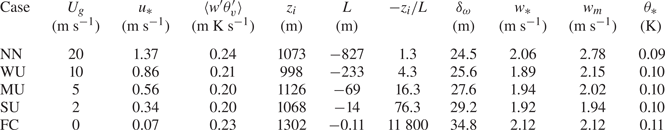
Table 1. Main characteristic parameters of each simulation, including the geostrophic wind  $U_g$ (
 $V_g=0$), the friction velocity
  $u_*$, the buoyancy flux
  $\langle w' \theta _v' \rangle$, the ABL depth
  $z_i$ where, these
  $z_i$ values are calculated using the ’maximum vertical gradient method’ (Sullivan et al. Reference Sullivan, Moeng, Stevens, Lenschow and Mayor1998) using virtual potential temperature as the scalar, the Obukhov length
  $L$, the vorticity thickness at canopy top
  $\delta _\omega$, the convective velocity scale
  $w_*$, the mixed velocity scale
  $w_m$ and the potential temperature scale
  $\theta _*$ (adapted from Patton et al. Reference Patton, Sullivan, Shaw, Finnigan and Weil2016).

2.4. Multi-level filtering and budget equations
2.4.1. Multi-level filtering formalism
A brief overview of the multi-level (or multi-resolution) approach is given in this section, the reader being referred to the monograph of Sagaut et al. (Reference Sagaut, Deck and Terracol2013) for extensive details. The general idea of this approach is that representations of any variable at coarser and coarser spatial resolution can be obtained by the successive application of scale separation filters. An illustration of such a decomposition is shown in figure 2 when applied using sharp cutoff filters in wavenumber space.
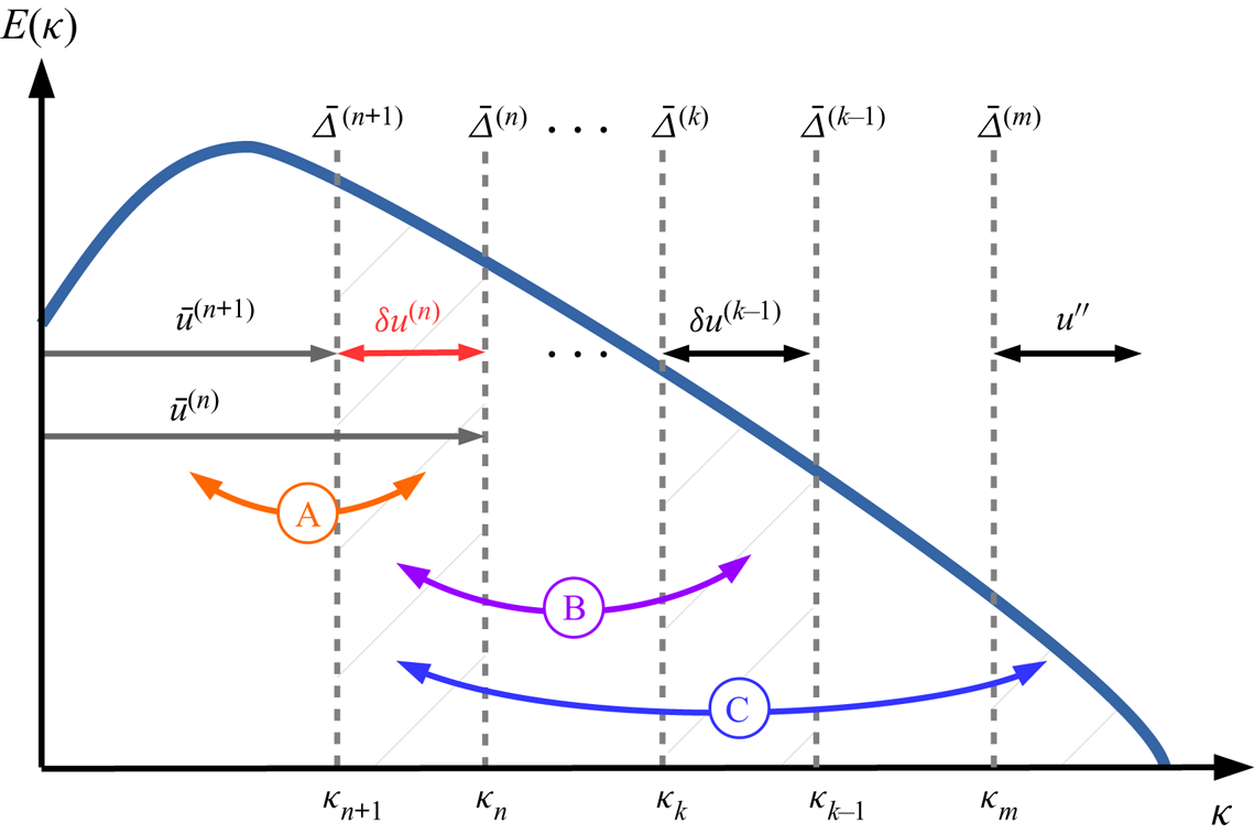
Figure 2. Multi-level decomposition of the variable  $u$ shown in spectral space in the case of sharp cutoff filters, depicting interactions between
  $\delta u^{(n)}=\bar {u}^{(n+1)}-\bar {u}^{(n)}$ and: (A) the larger scales
  $u^{(n+1)}$ via the term
  ${\mathcal {L}}_{ij}^{(n+1)}$, (B) a spectral band
  $\delta u^{(m)}$ at some smaller scale (
 $m< n$) via the term
  $\sum _{k=m+1}^{n-1}({\mathcal {G}}_{k+1}^{(n+1)}-{\mathcal {G}}_{k+1}^{(n)}){\mathcal {L}}_{ij}^{(k)}$, (C) all the scales
  $u''$ smaller than the LES-filter scale
  $\bar {\varDelta }^{(m)}$ via the term
  $({\mathcal {G}}_{m+1}^{(n+1)}-{\mathcal {G}}_{k+1}^{(n)})T_{ij}^{(m)}$ (adapted from Sagaut et al. Reference Sagaut, Deck and Terracol2013). The definition and derivation of the terms
  ${\mathcal {L}}_{ij}^{(n)}$ and
  $T_{ij}^{(m)}$ can be found in Appendix A.2.
Let  $G_n$ represent a hierarchy of filtering operators characterized by their respective cutoff length scales
  $\bar {\varDelta }^{(n)}$, such that
  $\bar {\varDelta }^{(n+1)} > \bar {\varDelta }^{(n)}$. Successive application of the primary filters
  $G_m$ to
  $G_n$ with cutoff length scales ranging from
  $\bar {\varDelta }^{(m)}$ to
  $\bar {\varDelta }^{(n)}$ (
 $m< n$), respectively, results in a filtering operator
  ${\mathcal {G}}_m^n$:
 \begin{equation} {\mathcal{G}}_m^n = G_n \star G_{n-1} \star \cdots\star G_{m+1} \star G_m, \end{equation}
where  $\star$ denotes the convolution product (
 $\bar {f}=G \star f$). The operator
  ${\mathcal {G}}_m^n$ has the following properties:
  ${\mathcal {G}}_n^n = G_n$ and
  ${\mathcal {G}}_0^0 = I$. With these notations, the classical (one-level) three-dimensional LES filter corresponds to
  $\bar {f} = G_1 \star f={\mathcal {G}}_1^1 \star f={\mathcal {G}}_0^1 \star f$ (with
  $f^{\prime \prime } = f-\bar {f}$ being the SFS component). Note that, in the present case, the LES spatial filter is an explicitly applied sharp filter in the horizontal and an implicit top-hat filter in the vertical (Sullivan & Patton Reference Sullivan and Patton2011). In the general case, the velocity field
  ${\boldsymbol u}$ can therefore be filtered
  $n$ times to obtain its representation at a coarse spatial resolution
 \begin{equation} \bar{{\boldsymbol u}}^{(n)} = {\mathcal{G}}_1^n \star {\boldsymbol u} = G_n \star G_{n-1} \star \cdots\star G_1 \star {\boldsymbol u}. \end{equation}
The variable  $\bar {{\boldsymbol u}}^{(n)}$ filtered at level
  $n$ represents the flow fields associated with wavenumbers
  $\kappa < \kappa _n$ with
  $\kappa _n = 2{\rm \pi} / \bar {\varDelta }^{(n)}, \bar {\varDelta }^{(n)}$ being the effective cutoff length scale of the hierarchical filters
  ${\mathcal {G}}_1^n$. With this approach, it is straightforward to define the band-pass filtered velocity:
  $\delta \bar {{\boldsymbol u}}^{(l)} = \bar {{\boldsymbol u}}^{(l)}-\bar {{\boldsymbol u}}^{(l+1)}$ which represents the fraction of the velocity field containing flow structures with a size smaller than
  $\bar {\varDelta }^{(l+1)}$ and larger than
  $\bar {\varDelta }^{(l)}$, e.g. the scales resolved at level
  $l$ and unresolved at level
  $l+1$. The particular case of standard LES, e.g. with only one filtering level (
 $n=1$) leads to:
  $\bar {{\boldsymbol u}}^{(1)} = \bar {{\boldsymbol u}}^{(n)}+ \sum _{l=1}^{n-1} \delta {\boldsymbol u}^{(l)}$ with
  ${\boldsymbol u}^{\prime \prime }$ being the SFS (unresolved) scales.
2.4.2. Multi-level filtered momentum transport equations
The multi-level filtering approach is applied here on the momentum transport equations as used in the present case (see (2.5)), which include the Coriolis, buoyancy and canopy-drag influence). The scale separation operator  ${\mathcal {G}}_1^{n}$ associated with the representation level
  $n$ is applied directly to the set of the Navier–Stokes equations (2.5), which becomes
 \begin{equation} \frac{\partial \bar{{\boldsymbol u}}^{(n)}}{\partial t} \!+\! \bar{{\boldsymbol u}}^{(n)} \boldsymbol{\cdot} \boldsymbol{\nabla} \bar{{\boldsymbol u}}^{(n)} ={-}f \hat{{\boldsymbol k}} \times (\bar{{\boldsymbol u}}^{(n)} \!-\! \bar{\boldsymbol U}_g^{(n)}) -\boldsymbol{\nabla} \bar{\rm \pi}^{(n)} + \hat{{\boldsymbol k}} \beta (\bar{\theta}_v^{(n)} - \theta_{v_0}) \!-\boldsymbol{\nabla} \boldsymbol{\cdot} {\boldsymbol T}^{(n)} + \bar{{\boldsymbol F}}_d^{(n)},\end{equation}
or, equivalently, with a more condensed presentation
 \begin{equation} \frac{\partial \bar{{\boldsymbol u}}^{(n)}}{\partial t} + \bar{{\boldsymbol u}}^{(n)} \boldsymbol{\cdot} \boldsymbol{\nabla} \bar{{\boldsymbol u}}^{(n)} = \bar{\boldsymbol L}^{(n)} -\boldsymbol{\nabla} \boldsymbol{\cdot} {\boldsymbol T}^{(n)} + \bar{{\boldsymbol F}}_d^{(n)},\end{equation}
where the term  ${\boldsymbol T}^{(n)}$ represents the ‘sub-level’ tensor (similar to the SFS tensor), including the influence of the unresolved and the resolved scales (up to the
  $n$th level) on the filtered field
  $\bar {{\boldsymbol u}}^{(n)}$
 \begin{equation} {\boldsymbol T}^{(n)} =\overline{{\boldsymbol u} \otimes {\boldsymbol u}}^{(n)} - \bar{\boldsymbol u}^{(n)} \otimes \bar{\boldsymbol u}^{(n)}, \end{equation}
and  $\bar {{\boldsymbol L}}^{(n)}$ represents the (linear) influence of pressure, buoyancy and Coriolis forces
 \begin{equation} \bar{\boldsymbol L}^{(n)} ={-}f \hat{{\boldsymbol k}} \times (\bar{{\boldsymbol u}}^{(n)} - \bar{\boldsymbol U}_g^{(n)}) -\boldsymbol{\nabla} \bar{\rm \pi}^{(n)} + \hat{{\boldsymbol k}} \beta (\bar{\theta}_v^{(n)} - \theta_{v_0}). \end{equation}
Subtracting (2.12) written at level  $n+1$ from (2.12) written at level
  $n$, one can obtain the evolution equation for the band-pass-filtered velocity
  $\delta {\boldsymbol u}^{(n)}= \bar {{\boldsymbol u}}^{(n)} - \bar {{\boldsymbol u}}^{(n+1)}$
 \begin{align} & \frac{\partial {\delta{\boldsymbol u}}^{(n)}}{\partial t} + \boldsymbol{\nabla} \boldsymbol{\cdot} ( {\delta{\boldsymbol u}}^{(n)} \otimes {\delta{\boldsymbol u}}^{(n)} +{\delta{\boldsymbol u}}^{(n)} \otimes \bar{{\boldsymbol u}}^{(n+1)} + \bar{{\boldsymbol u}}^{(n+1)}\otimes {\delta{\boldsymbol u}}^{(n)}) \nonumber\\ &\quad = \delta {\boldsymbol L}^{(n)} -\boldsymbol{\nabla} \boldsymbol{\cdot} ( {\boldsymbol T}^{(n)} -{\boldsymbol T}^{(n+1)} ) + ( \bar{{\boldsymbol F}}_d^{(n)} - \bar{{\boldsymbol F}}_d^{(n+1)} ), \end{align}
with  $\delta {\boldsymbol L}^{(n)} = \bar {\boldsymbol L}^{(n)}-\bar {\boldsymbol L}^{(n+1)}$. The calculation of the term
  $({\boldsymbol T}^{(n)} -{\boldsymbol T}^{(n+1)})$ using the multi-level filtering approach and the interpretation of its different contributions are detailed in Appendix A.2.
As detailed in Appendix A.3, at level  $n$, the drag force can be decomposed into
 \begin{equation} \bar{{\boldsymbol F}}_d^{(n)} = \boldsymbol{ D}^{(n)}+ \boldsymbol{ d}^{(n)}, \end{equation}
with  $\boldsymbol {D}^{(n)}=-c_d a \overline {v_w}^{(n)} \bar {{\boldsymbol u}}^{(n)}$ (with
  $c_d$ assumed constant, e.g. not scale dependent) being the contribution of the velocity filtered at level
  $(n$) and
  $\boldsymbol {d}^{(n)}$ the contribution of the velocity at filtering levels finer than
  $(n)$ to the drag at level
  $(n)$.
The momentum transport equation therefore reads
 \begin{align} &\frac{\partial {\delta{\boldsymbol u}}^{(n)}}{\partial t} + \boldsymbol{\nabla} \boldsymbol{\cdot} ( {\delta{\boldsymbol u}}^{(n)} \otimes {\delta{\boldsymbol u}}^{(n)} +{\delta{\boldsymbol u}}^{(n)} \otimes \bar{{\boldsymbol u}}^{(n+1)} + \bar{{\boldsymbol u}}^{(n+1)}\otimes {\delta{\boldsymbol u}}^{(n)})\nonumber\\ &\quad = \delta {\boldsymbol L}^{(n)} -\boldsymbol{\nabla} \boldsymbol{\cdot} ( {\boldsymbol T}^{(n)} -{\boldsymbol T}^{(n+1)} ) + ( \boldsymbol{D}^{(n)}- \boldsymbol{D}^{(n+1)}) + (\boldsymbol{ d}^{(n)}-\boldsymbol{ d}^{(n+1)} ). \end{align}
2.4.3. Transport equation of the TKE and Reynolds stress of $\delta {\boldsymbol{u}}^{(n)}$

With the above drag decomposition, the transport equation of the momentum associated with the band-pass-filtered velocity  $\delta {\boldsymbol{u}}^{(n)}$ reads with index notation (from (2.17))
 \begin{align} &\frac{\partial {\delta u}_i^{(n)}}{\partial t} +\frac{\partial}{\partial x_j} ( {\delta u}_i^{(n)} {\delta u}_j^{(n)} +{\delta u}_i^{(n)} {\bar{u}}_j^{(n+1)} + {\bar{u}}_i^{(n+1)} {\delta u}_j^{(n)}) \nonumber\\ &\quad = \delta {L}_i^{(n)} -\frac{\partial}{\partial x_j} ( {T}_{ij}^{(n)} -{T}_{ij}^{(n+1)} ) + ( {{D}}_{i}^{(n)}- {{D}}_{i}^{(n+1)}) + ({d}_{i}^{(n)}-{d}_{i}^{(n+1)} ). \end{align}
In order to derive the transport equation of the TKE of  $\delta {\boldsymbol{u}}^{(n)}$, this equation is written for the component
  $\delta {u}_\alpha ^{(n)}$, multiplied by
  $\delta {u}_\alpha ^{(n)}$, followed by a contraction over the repeated index
  $\alpha$. The transport equation of
  $\delta$KE
 $^{(n)}=\frac {1}{2}\delta _\alpha ^{(n)}\delta _\alpha ^{(n)}$, the kinetic energy of
  $\delta {\boldsymbol{u}}^{(n)}$, reads
 \begin{align} \frac{\partial}{\partial
t} (\frac{1}{2}{\delta u}_\alpha^{(n)}{\delta
u}_\alpha^{(n)}) & ={-} \frac{\partial}{\partial x_j}
\left( \frac{1}{2}{\delta u}_\alpha^{(n)}{\delta
u}_\alpha^{(n)} {\delta u}_j^{(n)} +\frac{1}{2}{\delta
u}_\alpha^{(n)}{\delta u}_\alpha^{(n)} {\bar{u}}_j^{(n+1)}\right)
\nonumber\\
&\quad -{\delta u}_\alpha^{(n)}{\delta u}_j^{(n)}\frac{{\partial\bar{u}}_\alpha^{(n+1)}}{\partial x_j} + \delta {L}_\alpha^{(n)}{\delta u}_\alpha^{(n)}
\nonumber\\ &\quad +( {T}_{\alpha\beta}^{(n)}
-{T}_{\alpha\beta}^{(n+1)} ) \frac{\partial {\delta
u}_\alpha^{(n)}}{\partial x_\beta}
-\frac{\partial}{\partial x_\beta} (
({T}_{\alpha\beta}^{(n)} -{T}_{\alpha\beta}^{(n+1)}){\delta
u}_\alpha^{(n)} )\nonumber\\ &\quad - a c_d (
\delta{v_w}^{(n)}{\delta{u}}_\alpha^{(n)}{\delta
u}_\alpha^{(n)} +\delta{v_w}^{(n)}{\delta
u}_\alpha^{(n)}{\bar{u}}_\alpha^{(n+1)}
+{\overline{v_w}}^{(n+1)}{\delta u}_\alpha^{(n)}{\delta
u}_\alpha^{(n)}) \nonumber\\ & \quad +
({d}_\alpha^{(n)}-{d}_\alpha^{(n+1)} ){\delta
u}_\alpha^{(n)}.
\end{align}
\begin{align} \frac{\partial}{\partial
t} (\frac{1}{2}{\delta u}_\alpha^{(n)}{\delta
u}_\alpha^{(n)}) & ={-} \frac{\partial}{\partial x_j}
\left( \frac{1}{2}{\delta u}_\alpha^{(n)}{\delta
u}_\alpha^{(n)} {\delta u}_j^{(n)} +\frac{1}{2}{\delta
u}_\alpha^{(n)}{\delta u}_\alpha^{(n)} {\bar{u}}_j^{(n+1)}\right)
\nonumber\\
&\quad -{\delta u}_\alpha^{(n)}{\delta u}_j^{(n)}\frac{{\partial\bar{u}}_\alpha^{(n+1)}}{\partial x_j} + \delta {L}_\alpha^{(n)}{\delta u}_\alpha^{(n)}
\nonumber\\ &\quad +( {T}_{\alpha\beta}^{(n)}
-{T}_{\alpha\beta}^{(n+1)} ) \frac{\partial {\delta
u}_\alpha^{(n)}}{\partial x_\beta}
-\frac{\partial}{\partial x_\beta} (
({T}_{\alpha\beta}^{(n)} -{T}_{\alpha\beta}^{(n+1)}){\delta
u}_\alpha^{(n)} )\nonumber\\ &\quad - a c_d (
\delta{v_w}^{(n)}{\delta{u}}_\alpha^{(n)}{\delta
u}_\alpha^{(n)} +\delta{v_w}^{(n)}{\delta
u}_\alpha^{(n)}{\bar{u}}_\alpha^{(n+1)}
+{\overline{v_w}}^{(n+1)}{\delta u}_\alpha^{(n)}{\delta
u}_\alpha^{(n)}) \nonumber\\ & \quad +
({d}_\alpha^{(n)}-{d}_\alpha^{(n+1)} ){\delta
u}_\alpha^{(n)}.
\end{align}
A detailed interpretation of the different terms in (2.19) is given in § B.2.
The transport equation for  $\delta \textrm {RS}_{ij}^{(n)}$ the Reynolds stress
  $(\delta u_i^{(n)} \delta u_j^{(n)})$ is obtained by adding the transport equation (2.18) of
  $\delta u_i^{(n)}$ multiplied by
  $\delta u_j^{(n)}$ to the transport equation (2.18) of
  $\delta u_j^{(n)}$ multiplied by
  $\delta u_i^{(n)}$. The sub-level Reynolds stress transport equation therefore reads
 \begin{align}
\frac{\partial }{\partial t} ({\delta u}_i^{(n)}{\delta u}_j^{(n)}) &
={-}\frac{\partial}{\partial x_\alpha} (({\delta u}_i^{(n)} {\delta u}_j^{(n)}) {\delta u}_\alpha^{(n)}
+({\delta u}_i^{(n)} {\delta u}_j^{(n)}){\bar{u}}_\alpha^{(n+1)})\nonumber\\
& \quad -\left({\delta u}_j^{(n)}{\delta u}_{\alpha}^{(n)}\frac{\partial{\bar{u}}_i^{(n+1)}}{\partial x_{\alpha}} +{\delta
u}_i^{(n)}{\delta u}_{\alpha}^{(n)} \frac{\partial{\bar{u}}_j^{(n+1)}}{{\partial x_{\alpha}}}\right)\nonumber\\
& \quad + ( {\delta u}_j^{(n)} \delta
{L}_i^{(n)} + {\delta u}_i^{(n)}\delta
{L}_j^{(n)})\nonumber\\ &\quad + ( {T}_{i\alpha}^{(n)}
-{T}_{i\alpha}^{(n+1)} ) \frac{\partial {\delta
u}_j^{(n)}}{\partial x_\alpha} + ( {T}_{j\alpha}^{(n)}
-{T}_{j\alpha}^{(n+1)} ) \frac{\partial {\delta
u}_i^{(n)}}{\partial x_\alpha}\nonumber\\ & \quad -
\frac{\partial }{\partial x_\alpha} ( ({T}_{i\alpha}^{(n)}
-{T}_{i\alpha}^{(n+1)}){\delta u}_j^{(n)}
+({T}_{j\alpha}^{(n)} -{T}_{j\alpha}^{(n+1)}){\delta
u}_i^{(n)}) \nonumber\\ & \quad - a c_d ( 2 {\delta
u}_i^{(n)} {\delta u}_j^{(n)} [{\delta
v_w}^{(n)}+\overline{v_w}^{(n+1)}]\nonumber\\ & \quad
+{\delta v_w}^{(n)} [ \bar{u}_{i}^{(n+1)}{\delta u}_j^{(n)}
+ \bar{u}_{j}^{(n+1)}{\delta u}_i^{(n)}]) \nonumber\\
&\quad + ({d}_{i}^{(n)}-{d}_{i}^{(n+1)} ){\delta u}_j^{(n)}
+ ({d}_{j}^{(n)}-{d}_{j}^{(n+1)} ){\delta
u}_i^{(n)}. \end{align}
\begin{align}
\frac{\partial }{\partial t} ({\delta u}_i^{(n)}{\delta u}_j^{(n)}) &
={-}\frac{\partial}{\partial x_\alpha} (({\delta u}_i^{(n)} {\delta u}_j^{(n)}) {\delta u}_\alpha^{(n)}
+({\delta u}_i^{(n)} {\delta u}_j^{(n)}){\bar{u}}_\alpha^{(n+1)})\nonumber\\
& \quad -\left({\delta u}_j^{(n)}{\delta u}_{\alpha}^{(n)}\frac{\partial{\bar{u}}_i^{(n+1)}}{\partial x_{\alpha}} +{\delta
u}_i^{(n)}{\delta u}_{\alpha}^{(n)} \frac{\partial{\bar{u}}_j^{(n+1)}}{{\partial x_{\alpha}}}\right)\nonumber\\
& \quad + ( {\delta u}_j^{(n)} \delta
{L}_i^{(n)} + {\delta u}_i^{(n)}\delta
{L}_j^{(n)})\nonumber\\ &\quad + ( {T}_{i\alpha}^{(n)}
-{T}_{i\alpha}^{(n+1)} ) \frac{\partial {\delta
u}_j^{(n)}}{\partial x_\alpha} + ( {T}_{j\alpha}^{(n)}
-{T}_{j\alpha}^{(n+1)} ) \frac{\partial {\delta
u}_i^{(n)}}{\partial x_\alpha}\nonumber\\ & \quad -
\frac{\partial }{\partial x_\alpha} ( ({T}_{i\alpha}^{(n)}
-{T}_{i\alpha}^{(n+1)}){\delta u}_j^{(n)}
+({T}_{j\alpha}^{(n)} -{T}_{j\alpha}^{(n+1)}){\delta
u}_i^{(n)}) \nonumber\\ & \quad - a c_d ( 2 {\delta
u}_i^{(n)} {\delta u}_j^{(n)} [{\delta
v_w}^{(n)}+\overline{v_w}^{(n+1)}]\nonumber\\ & \quad
+{\delta v_w}^{(n)} [ \bar{u}_{i}^{(n+1)}{\delta u}_j^{(n)}
+ \bar{u}_{j}^{(n+1)}{\delta u}_i^{(n)}]) \nonumber\\
&\quad + ({d}_{i}^{(n)}-{d}_{i}^{(n+1)} ){\delta u}_j^{(n)}
+ ({d}_{j}^{(n)}-{d}_{j}^{(n+1)} ){\delta
u}_i^{(n)}. \end{align}
2.4.4. Terms investigated in analysing the $\boldsymbol{{u}}^L$ – $\boldsymbol{{u}}^S$ interaction


Horizontally and time averaging (2.19) and (2.20) along with computing the standard deviation of each term of their right-hand side not only allows for the estimation of the mean TKE or Reynolds shear stress (RSS) transport between scales via different mechanisms (e.g. spatial transport and interscale energy transfer) but also the quantification of their instantaneous (or local) intensity. In particular, comparing the standard deviation magnitude to that of the average quantity is a way to identify the existence of both forward and backscatter of energy among scales (e.g. an instantaneous two-way coupling between scales). Since the present study focuses on the interaction between the (large) ABL scales and the (small) canopy scales, only a few terms from (2.19) or (2.20) are analysed. The detail of their derivation for a four-level decomposition (as in (2.1)) is given in Appendix D. For the sake of comparison, the term  $B^S$ corresponding to the contribution of buoyancy to the small-scale TKE or RSS is included. The terms of focus are presented and defined in table 2 and are represented schematically in figure 3. They are selected to guide interpretation of the small-scale TKE budget of
  $(\xi ^S)^2 = \frac {1}{2}u_\alpha ^S u_\alpha ^S = \delta$KE
 $^{(1)}$. For the Reynolds shear stress budget, the same notations are employed for consistency. An analysis of the statistical error of these terms is presented in Appendix E.2.
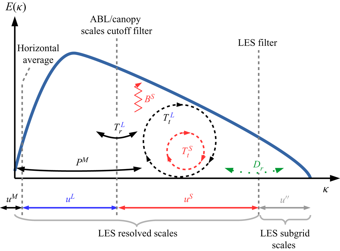
Figure 3. Four-level decomposition shown in spectral space depicting the budget terms for  $(\xi ^S)^2$ the (small) canopy-scale TKE, as listed in table 2. The terms representing the spatial transport of
  $(\xi ^S)^2$ by
  $u^S$ and
  $u^L$ (labelled
  $T_t^S$ and
  $T_t^L$, respectively), are shown with dashed line circles, the production of
  $(\xi ^S)^2$ by the mean flow
  $P^M$ and the interscale transfer of TKE between
  $u^S$ and
  $u^L$ (labelled
  $T_r^L$) are shown with solid line arrows, the influence of canopy drag
  $D_r$ is shown with a dotted line arrow and the production of
  $(\xi ^S)^2$ by buoyancy (labelled
  $B^S$) is shown with a zig-zag arrow. Vertical dashed lines sketch the different cutoff filters involved in the four-level decomposition: the LES filter, the cutoff filter employed to separate the resolved scales
  $u^L$ and
  $u^S$ and the horizontal averaging operation.
Table 2. Budget terms for  $(\xi ^S)^2= \frac {1}{2} [(u^S)^2+(v^S)^2+(w^S)^2]$ the small-scale TKE investigated in the present study. Equivalent terms for the small-scale RSS are calculated as well (see Appendix D.2).
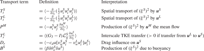
3. Results
In the following, the symbol  $\bar {\ }$, denoting the LES filter, is dropped for simplicity. All presented quantities are based on the resolved velocity field.
3.1. Statistics
As both an in-depth statistical description of the canopy flow and a validation against the literature have already been presented by Patton et al. (Reference Patton, Sullivan, Shaw, Finnigan and Weil2016), only a brief overview of the main characteristics of the ABL flow developing over a vegetation canopy is given here.
The mean vertical structure of the simulated ABLs is characterized in figure 4 using vertical profiles of key statistical quantities such as the mean horizontal velocity, mean potential temperature, resolved heat flux, variance of the horizontal and vertical velocity components and the RSS  $\langle u'w' \rangle$. Above the canopy, all the statistics of the present configuration are in very good agreement with those recently reported by Salesky & Anderson (Reference Salesky and Anderson2018) for similar values of
  $-z_i/L$. For brevity, only the characteristics of the weakly unstable (WU,
  $-z_i/L=4.3$) are discussed here. Statistical error of these statistics are presented in Appendix E.1. The horizontal wind speed shows a gradual increase with height while the mean potential temperature shows a decrease up to
  $z/z_i = 0.7$, in agreement with the imposed stability regime. However, inside the canopy, the vertical profile of the horizontal wind speed shows an inflection point near the top of canopy (Patton et al. Reference Patton, Sullivan, Shaw, Finnigan and Weil2016), in agreement with the now well-admitted presence of the shear-layer flow developing at canopy top. Consistent with the results of Salesky & Anderson (Reference Salesky and Anderson2018), both the variance of the horizontal wind speed and the resolved heat flux exhibit a monotonic decrease in the region up to
  $z/z_i=0.7$. However, given the finer spatial resolution of the present simulations and the presence of the canopy, these two statistics show a local maximum just above canopy top and a subsequent reduction with decreasing
  $z$. These two statistics show a decrease below canopy top with also an inflection point in their vertical profiles. As noted by Salesky & Anderson (Reference Salesky and Anderson2018), the vertical evolution of the variance of the wall-normal velocity component is more complex with first a local maximum close to canopy top at
  $z/z_i=0.04$ or
  $z/h=2$, a slight decrease followed by an increase with an absolute maximum at
  $z/z_i=0.4$. Above
  $z/z_i=0.4, \langle {w^\prime }^2\rangle /w_m^2$ shows a gradual decrease. The local extremum at the lowest location can be attributed to influence of the canopy and the associated strong shear and turbulence production while the gradual increase up to
  $z/z_i=0.4$ is an already observed feature of sheared convective boundary layers caused by TKE redistribution among velocity components (see Salesky & Anderson (Reference Salesky and Anderson2018) and references therein). The RSS shows negative values throughout the ABL with an extremum at canopy top and a gradual decrease in magnitude with increasing wall-normal distance. Combined with the wall-normal profile of the horizontal velocity which exhibits high shear at the same location, it indicates that the near-canopy region is a region of strong production of kinetic turbulent energy. Finally, in agreement with the literature, the skewness of the streamwise and wall-normal velocity components (not shown here) show negative and positive values, respectively, above the canopy, corresponding to the presence of strong ejection events. Within the canopy, streamwise and vertical velocity skewness shift to positive and negative values, respectively, consistent with the statistical predominance of strong sweeping events in this region (Patton et al. Reference Patton, Sullivan, Shaw, Finnigan and Weil2016).
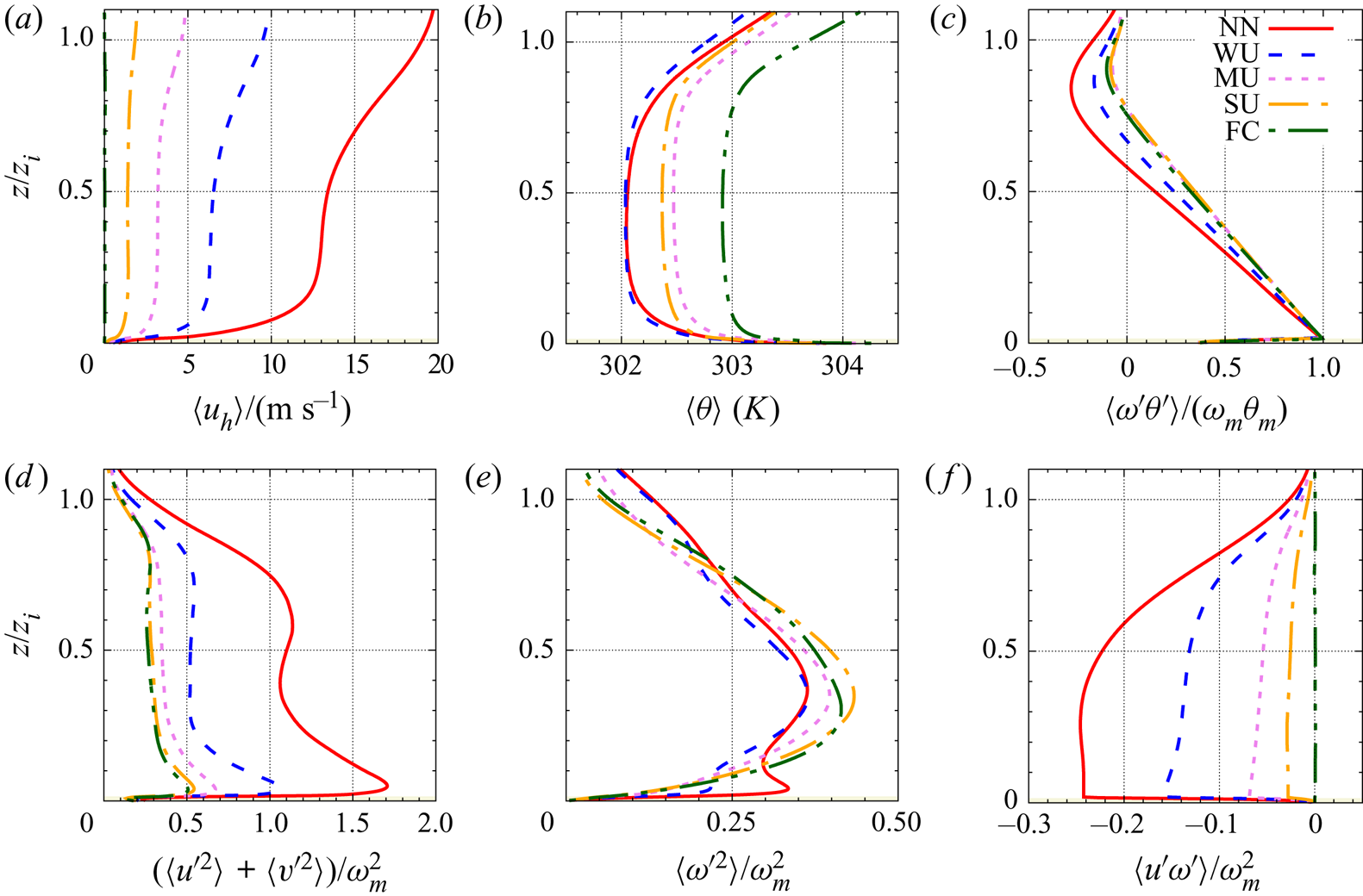
Figure 4. Horizontal ensemble-averaged wall-normal profiles of  $(a)$ horizontal wind speed
  $\langle u_h \rangle = (\langle u \rangle ^2 +\langle v\rangle ^2)^{1/2}$,
  $(b)$ temperature
  $\langle \theta \rangle$,
  $(c)$ resolved heat flux
  $\langle w^\prime \theta ^\prime \rangle /(w_m \theta _m)$,
  $(d)$ horizontal velocity variance
  $(\langle {u^\prime }^2 \rangle +\langle {v^\prime }^2\rangle )/w_m^2$,
  $(e)$ vertical velocity variance
  $\langle {w^\prime }^2 \rangle /w_m^2$ and
  $(f)$ RSS
  $\langle u^\prime w^\prime \rangle /w_m^2$ for all the cases (the WU case is shown in blue dashed lines).
3.2. Flow visualization
Instantaneous horizontal slices of the three velocity component fluctuations  $u^\prime , v^\prime$ and
  $w^\prime$ normalized by
  $w_m$ at
  $z/h=$ 10, 5 and 1 (
 $z/z_i=$ 0.20, 0.10 and 0.02, respectively) are presented in figure 5(
 $a$–
$a$– $i$) with close up views of the lowest level in figure 5(
 $j$,
$j$, $k$,
$k$, $l$) for the WU case. Well above the canopy (figure 5
 $a$–
$a$– $f$), the fluctuations of the three velocity components are marked by the presence of large-scale structures elongated in the streamwise direction. Regions of narrow intense upward motion (figure 5
 $c$,
$c$, $f$) are found to correspond to narrow streaks of low longitudinal velocity (figure 5
 $a$,
$a$, $d$) and region of lateral convergence of the flow (figure 5
 $b$,
$b$, $e$). Conversely, the regions of downdraft are broader, their locations match that of the high longitudinal velocity regions and correspond to region of lateral divergence of the flow. These structures are separated in the transverse direction by a distance on the order of
  $z_i$, which corresponds well to the presence of large convective rolls of streamwise axis (Lemone Reference Lemone1973). In the present study, the main axis of the convective rolls is oriented along the streamwise direction
  $x$ whereas observations reported that their axis is usually at an angle of about 20
 $^{\circ }$ from the ABL layer-average wind direction (Lemone Reference Lemone1973). It should be noted that smaller scales are embedded in these large-scale structures, and are likely to be under the influence of the larger scales as observed by Lemone (Reference Lemone1976) and recently confirmed by Patton et al. (Reference Patton, Sullivan, Shaw, Finnigan and Weil2016) and Salesky & Anderson (Reference Salesky and Anderson2018). At the top of the canopy (
 $z/h = 1$),
  $w'$ does not show the footprint of large structures scaling with
  $z_i$ but rather a finer-scale organization (figure 5
 $i$). Examination of the close up view (figure 5
 $l$) reveals the presence of both intense localized downdraft motions and weaker and broader updraft motions. At this wall-normal distance, the streamwise velocity
  $u'$ exhibits more anisotropic structures than
  $w'$, showing streaks of low- and high-speed elongated in the streamwise direction. Looking at the entire
  $x$–
$x$– $y$ plane (figure 5
 $g$), narrow long low-speed streaks can be seen. Their locations match well that of the low streamwise velocity regions detected
  $z/h =$ 5 and 10 (figure 5
 $a$,
$a$, $d$). Inspection of
  $v'$ reveals a strong imprint of the larger scales detected at higher levels, with embedded smaller scales resembling oblique streaks of negative and positive lateral velocity.
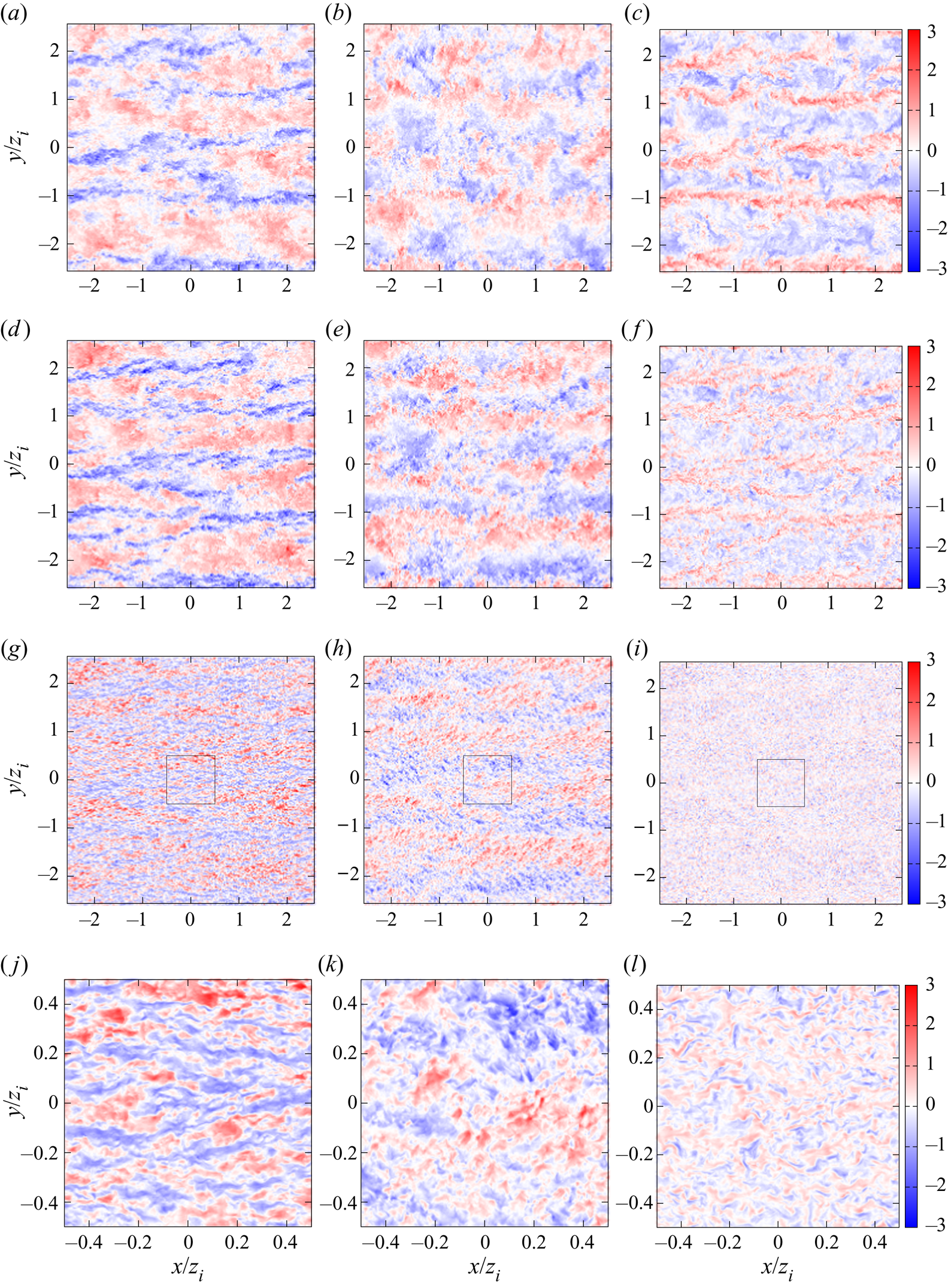
Figure 5. Instantaneous fluctuations normalized by  $w_m$ of (left)
  $u$, (centre)
  $v$ and (right)
  $w$ in the
  $x$–
$x$– $y$ plane at (
 $a$,
$a$, $b$,
$b$, $c$)
$c$)  $z/h=10$, (
 $d$,
$d$, $e$,
$e$, $f$)
$f$)  $z/h=5$ and (
 $g$,
$g$, $h$,
$h$, $i$)
$i$)  $z/h=1$ for the WU case. Panels (
 $j$,
$j$, $k$,
$k$, $l$) are close up views of the centre of the velocity field at
  $z/h=1$ corresponding to the black squares shown in (
 $g$,
$g$, $h$,
$h$, $i$).
$i$).
From these qualitative observations, it can be concluded that the flow near the canopy top results from the superposition of large scales (of size of the order of  $z_i$) onto smaller scales, with size of the order of
  $h$. This is in agreement with the observations of Raupach et al. (Reference Raupach, Finnigan and Brunet1996) and Patton et al. (Reference Patton, Sullivan, Shaw, Finnigan and Weil2016) that canopy eddies (consisting of compact strong intermittent sweeps and large weaker ejections) are under the influence of larger scales of the ABL, whose structure in the present case seems compatible with the presence of convective rolls. Longitudinal spacing of the structures present in the canopy-top region is also in qualitative agreement with the estimate
  $\varLambda _x/ L_s = 8.1$ of Raupach et al. (Reference Raupach, Finnigan and Brunet1996) which corresponds here to
  $5.2h$. It is worth mentioning that near canopy top, the presence of the larger scales of the ABL is mainly seen in both
  $u'$ and
  $v'$, the latter being likely to play a major role in generating canopy-eddies through the triggering of Kelvin–Helmholtz instabilities, despite leaving no trace in the statistics because of the homogeneous character of the flow in the lateral direction
  $y$.
$y$.
3.3. Spectrograms
The qualitative conclusions based on the instantaneous slices presented in § 3.2 are now further investigated for the WU case through the analysis of the premultiplied one-dimensional spectra of the three velocity components, as a function of height  $z$ and the spatial longitudinal or transverse wavelength,
  $\lambda _x$ or
  $\lambda _y$, respectively (figure 6). The wavelength corresponding to local maxima in the streamwise and transverse direction are denoted
  $\lambda _x^m$ and
  $\lambda _y^m$, respectively.
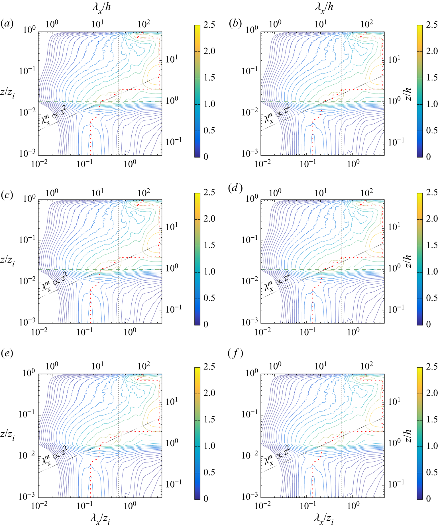
Figure 6. Pre-multiplied spectra of the three velocity components plotted as a function of the wall-normal distance  $z$ and (left) the streamwise wavelength
  $\lambda _x$ and (right) the transverse wavelength
  $\lambda _y$ (normalized by
  $z_i$ or
  $h$) (WU case). Pre-multiplied spectra normalized by
  $w_m^2$ of
  $u, v$ and
  $w$ are shown in (
 $a$,
$a$, $b$), (
 $c$,
$c$, $d$) and (
 $e$,
$e$, $f$), respectively. The vertical dashed line shows the cutoff wavelength chosen for scale separation. The red dashed line indicates the location of the local maximum of the spectra. Oblique dotted blacked lines correspond to trends
  $\lambda ^m \propto z^2$ in (
 $a$,
$a$, $c$,
$c$, $d$) and
  $\lambda ^m \propto z$ in (
 $b$,
$b$, $e$,
$e$, $f$) of the most energetic canopy scales in the region
  $1< z/h<5$. Spectra are scaled up by a factor of
  $10^4$ for clarity. For clarity, 20 contours are distributed logarithmically between 0.025 and the maximum of each spectrum. The horizontal dark-green long-dashed line corresponds to canopy top.
Within the canopy, the wavelengths corresponding to the maximum of energy of the longitudinal and transverse spectra of both  $u$ and
  $v$ are fairly constant with height, particularly in the lower half of the canopy (
 $0 < z/h < 0.5$). In this region of the canopy, the value of the wavelengths corresponding to the most energetic scales of the longitudinal component
  $u$ are found to be such that
  $\lambda ^m_x < \lambda ^m_y$. This might be interpreted as the footprint of the two-dimensional roller structures of spanwise axis generated by the Kelvin–Helmholtz instability at canopy top. However, the detailed investigation of the characteristics of the coherent structures within the canopy in beyond the scope of the present paper. Table 3 summarizes these wavelengths obtained in the upper half of the canopy. These length scales derived based upon the local spectral peak are larger than the integral length scales presented in Patton et al. (Reference Patton, Sullivan, Shaw, Finnigan and Weil2016), however, the length scale variation with wall-normal distance is consistent across both techniques. In the streamwise direction, the wavelength corresponding to the peak of the energy spectra of the vertical velocity component
  $w$ is constant throughout the canopy (
 $0< z/h<1$) and equal to
  $\lambda ^m_x/ h=4$, consistent with the integral length scales computed by Patton et al. (Reference Patton, Sullivan, Shaw, Finnigan and Weil2016). Conversely, in the transverse direction, the wavelengths of the most energetic structures increase with wall distance in the bottom half of the canopy and stays approximately constant in the upper half, with
  $\lambda ^m_y/ h\approx 4$ in this region. Finding similar values for
  $\lambda ^m_x$ and
  $\lambda ^m_y$ near canopy top confirms the isotropic character of the structures in
  $w$ noted in figure 5. In the streamwise direction,
  $\lambda _x / h=4$ corresponds to a streamwise spacing of canopy eddies
  $\varLambda _x / h=4$ (as defined by Raupach et al. Reference Raupach, Finnigan and Brunet1996) which falls into the range reported by Raupach et al. (Reference Raupach, Finnigan and Brunet1996) for comparable
  $L_s/h$ (
 $=0.64$ in the present case).
Table 3. Streamwise and spanwise wavelengths  $\lambda _x^m$ and
  $\lambda _y^m$ corresponding to the most energetic scales of the three velocity components in the different regions of the flow, normalized by the canopy height
  $h$ or the boundary-layer depth
  $z_i$.

It must be noted that, for the present WU stability regime, inside the canopy, footprint of the larger scales from the ABL is only visible in the spectra in the transverse direction of  $v$. Therefore, even if visible on instantaneous snapshots of the flow field, they are not energetic enough to stand out in this flow configuration. This contrasts with the spectral characteristics of the flow found in other stability regimes for which secondary peaks at ABL scales are present (Patton et al. Reference Patton, Sullivan, Shaw, Finnigan and Weil2016). However, further analysis is beyond the scope the present study. In the region
  $1< z/h<5$, all the spectra show a local maximum wavelength of the order of a few
  $h$ in agreement with the presence of canopy scales. Nevertheless, the primary spectral peak of the transverse velocity component corresponds to the larger scales from the ABL, which coexist with the canopy scale in this region. The wavelengths corresponding to the near-canopy structures increase with the wall distance either as
  $\lambda ^m \propto z^2$ for
  $u$ in the streamwise direction and
  $v$ in both directions or
  $\lambda ^m \propto z$ for
  $u$ in the transverse direction and
  $w$ in both directions (oblique dotted line in 6). In the region extending up to
  $z/h = 5$, the transverse wavelength corresponding to the local extrema of the pre-multiplied spectra of
  $w$ in the
  $x$ and
  $y$ directions shows a clear linear evolution with the wall-normal coordinate. This behaviour is also visible for the longitudinal component
  $u$, but only for the transverse direction. This linear increase with wall-normal distance of the most energetic scales is in agreement with the linear increase of the transverse spacing of low- and high-speed streaks and size of vortical structures reported in the surface layer of the ABL by previous studies (Lin et al. Reference Lin, McWilliams, Moeng and Sullivan1996a,Reference Lin, Moeng, Sullivan and McWilliamsb; Drobinski et al. Reference Drobinski, Carlotti, Newsom, Banta, Foster and Redelsperger2004).
Well above the canopy, the pre-multiplied spectra in the transverse direction reveal the presence of the footprint of large scales at  $\lambda _y/ z_i = 1.0$ below
  $0.15 z_i$ for
  $u$ and
  $v$ and above
  $0.15 z_i$ for
  $w$. The presence of this peak in the spectra in the outer region of the boundary layer is consistent with the existence of streamwise rolls of large vertical and spanwise extent, and at the bottom of which the vertical component is minimum. Moreover, the lateral spacing corresponding to this wavelength of
  $1.0 z_i$ is in agreement with the observations from figure 5. According to Sykes & Henn (Reference Sykes and Henn1989), when
  $u_{*}/w_{*}$ is between 0.35 and 0.5, the aspect ratio of the rolls (defined as their width divided by their depth) is approximately 4. Therefore, in the present simulation, the ratio
  $u_{*}/w_{*}$ being equal to 0.45, one could use the value of the roll lateral spacing given by the large-scale lateral wavelength of
  $1.0 z_i$ to estimate the vertical extent of these structures to be
  $0.26 z_i$. In the longitudinal direction, there is a strong imprint of the larger scales showing at the wavelength
  $\lambda _x /z_i = 3.5$ for the three velocity components. Above
  $z/h = 5$, most of the energy is contained in the wavelength such that
  $\lambda _y / z_i \simeq 1.0$. Thus, in this region, the energy content in the spectral domain is consistent with the presence of large-scale structures corresponding to streamwise-oriented rolls whose vertical and spanwise extent scale with
  $z_i$. Pre-multiplied cospectra between the vertical velocity component
  $w$ and the longitudinal velocity component
  $u$ or the potential temperature
  $\theta$ as a function of the wall-normal distance and
  $\lambda _x$ or
  $\lambda _y$ are shown in figure 7. These plots clearly demonstrate the spectral separation between the near-canopy turbulence and the most energetic large scales from the ABL. The characteristic wavelengths identified in the pre-multiplied spectra of the velocity components are confirmed as well as the linear increase of the energetic scales with the wall-normal distance, entailing the presence of self-similar eddies. It is worth mentioning here that, when multiplied by the vertical gradient of the mean streamwise velocity, the RSS cospectrum provides direct information on the contribution of the turbulent scales to TKE production. It can already be anticipated that in the near-canopy region, TKE production mostly comes from the canopy scales themselves.

Figure 7. Pre-multiplied cospectra plotted as a function of the wall-normal distance  $z$ and the (left) streamwise wavelength
  $\lambda _x$ and (right) the transverse wavelength
  $\lambda _y$ (normalized by
  $z_i$ or
  $h$) (WU case). The negative of the pre-multiplied cospectra of
  $w$ and
  $u$ (e.g. vertical momentum flux) normalized by
  $w_m^2$ are shown in (
 $a$,
$a$, $b$) and pre-multiplied cospectra of
  $w$ and
  $\theta$ (e.g. vertical heat flux) normalized by
  $w_m\theta _m$ are shown in (
 $c$,
$c$, $d$). The vertical dashed line shows the cutoff wavelength retained for scale separation. The red dashed line indicates the location of the local maximum of the spectra. Cospectra are scaled up by a factor of
  $10^4$ for clarity. For clarity, 20 contours are distributed logarithmically between 0.025 and the absolute maximum of each cospectra. The horizontal dark-green long-dashed line corresponds to canopy top.
3.4. Evidence of AM of small scales
In the previous section, we have shown that the most energetic structures in the canopy region and in the ABL are well separated in spectral space. Here, we demonstrate in the WU case the existence of AM of the canopy turbulence by the larger scales of the ABL using the same method as that proposed by Bandyopadhyay & Hussain (Reference Bandyopadhyay and Hussain1984). To do so, we use instantaneous  $u '$ at the centre of the spatial domain (
 $y/h = 0$), at
  $z/h = 1$. A two-dimensional low-pass filter with cutoff wavelengths of
  $\lambda _x /z_i = 0.57$ and
  $\lambda _y /z_i = 0.29$ is employed to decompose
  $u^\prime$ into its large- and small-scale components
  $u^L$ and
  $u^S$, respectively, such that
  $u^\prime = u^L + u^S$. The large-scale envelope
  $E^L(u^S)$ of the small-scale signal is then computed by low-pass filtering
  $(u^S)^2$ with the same cutoff wavelength (Basley et al. Reference Basley, Perret and Mathis2018). Example signals obtained via this scale decomposition are shown in figure 8. The similarity between
  $u^L$ and
  $E^L(u^S)$ is evident and their resemblance is confirmed by the significant level of correlation between the two signals; which for the present case, the correlation coefficient between these two signals is 0.7, which clearly indicates AM of canopy turbulence by large ABL scales, similar to that found by Mathis et al. (Reference Mathis, Hutchins and Marusic2009) in the near-wall region of a FPBL. In order to quantify the AM of the small scales by the large scales of the flow, the single point AM coefficient, defined as the correlation coefficient between the low-pass filtered envelope of a small-scale quantity
  $X^S$ and the large-scale velocity component
  $u_i^L$, measured at the same point, is computed as (Mathis et al. Reference Mathis, Hutchins and Marusic2009)
 \begin{equation} AM(u_i^L,X^S)= \frac{\langle u_i^L E^L(X^S) \rangle} {\sigma_{u_i^L} \sigma_{E^L(X^S)}}. \end{equation}
In order to fully characterize the AM mechanism,  $AM(u_i^L,X^S)$ is computed for all the velocity components but also for the small-scale kinetic energy defined as
  $(\xi ^S)^2=[(u^S)^2+(v^S)^2+(w^S)^2]/2 = \delta$KE
 $^{(1)}$. Consistent with previous studies of various types of wall-bounded flows (e.g. Talluru et al. Reference Talluru, Baidya, Hutchins and Marusic2014; Blackman & Perret Reference Blackman and Perret2016; Basley et al. Reference Basley, Perret and Mathis2018; Salesky & Anderson Reference Salesky and Anderson2018), all small-scale velocity components (and consequently the small-scale kinetic energy) are amplitude modulated by the large-scale velocity components (figure 9). The wall-normal distribution of the AM coefficients depends on the large-scale component considered, while for one given large-scale component, all the small-scale quantities are influenced in the same manner, as demonstrated by AM correlation coefficients with similar wall-normal variation and magnitude. When considering
  $AM(u^L,X^S)$ (figure 9
 $a$), we find positive values with a peak at canopy top, meaning that canopy-scale turbulence is amplified by high-intensity large-scale structures of the streamwise velocity component
  $u^L$.
  $AM(u^L,X^S)$ changes sign at
  $z/h=2$ (or
  $z/z_i=0.04$), a behaviour similar to that found by Salesky & Anderson (Reference Salesky and Anderson2018). Non-zero values of
  $AM(v^L,X^S)$ (figure 9
 $b$) result from having not performed any local rotation has been performed to align the horizontal velocity components with the mean wind direction at each height (as was done in Salesky & Anderson (Reference Salesky and Anderson2018), for instance). Despite that difference, in the region above the canopy and when taking into account the vertical displacement induced by the canopy, the present levels of
  $AM(u^L,X^S)$ compares well to Salesky & Anderson (Reference Salesky and Anderson2018) (not shown here). A similar trend is found for the large-scale wall-normal velocity component
  $AM(w^L,X^S)$ as for
  $AM(u^L,X^S)$, but with opposite sign (figure 9
 $c$). Contrary to what Salesky & Anderson (Reference Salesky and Anderson2018) observed in their ABL flow without canopy, significant negative values of
  $AM(w^L,X^S)$ are found in the canopy region for all three small-scale velocity components and kinetic energy. Canopy-scale turbulence is therefore suppressed when upward (positive
  $w^L$) LSM exists within the canopy, while enhancing turbulence in the region above the canopy.
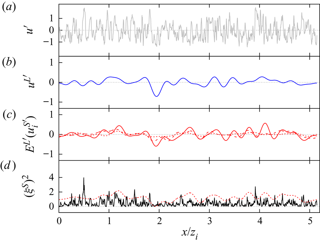
Figure 8. Instantaneous velocity signals showing AM at  $z/h=1$.
  $(a)$ instantaneous fluctuations
  $u^\prime$ of the streamwise velocity component,
  $(b)$ large-scale component of
  $u^\prime$,
  $(c)$ fluctuations of the low-pass-filtered envelope
  $E^L({u_i^\prime }^S)$ of the small-scale velocity components (solid line)
  ${u^\prime }^S$, (dashed line)
  ${v^\prime }^S$ and (dotted line)
  ${w^\prime }^S$,
  $(d)$ (solid black line) small-scale TKE
  $(\xi ^S)^2$ and (dotted red line) low-pass filtered envelope of
  $(\xi ^S)^2$. See text for the definition of the employed low-pass filter. (WU case).
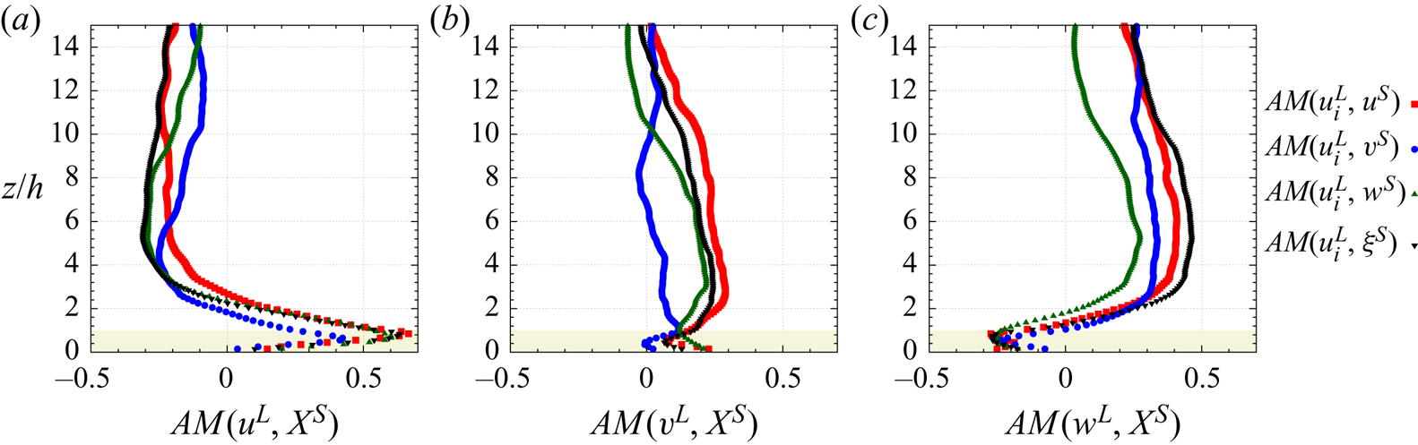
Figure 9. The AM coefficients of the three small-scale velocity components ( $\blacksquare$, red)
  $u^S$, (
 $\bullet$, blue)
  $v^S$, (
 $\blacktriangle$, green)
  $w^S$ and (
 $\blacktriangledown$, black) the corresponding TKE
  $(\xi ^S)^2$ by
  $(a)$ the large-scale streamwise velocity component
  $u^L$,
  $(b)$ the large-scale spanwise velocity component
  $v^L$ and
  $(c)$ the large-scale wall-normal velocity component
  $w^L$ (WU case). The beige shaded area corresponds to the canopy region.
3.5. Small-scale TKE and RSS budget
The transport equations for TKE and RSS obtained using the multi-level formalism presented in § 2.4 with a four-level decomposition are used to further analyse the interaction between large and small scales. Only the WU case is analysed here, the influence of atmospheric stability being addressed in § 3.6. We focus on terms representing interscale spatial transport and transfer of TKE and RSS between components of the velocity field (table 2), namely  $T_t^S$ the (spatial) turbulent transport of small-scale kinetic energy by the small scales themselves,
  $T_t^L$ the (spatial) turbulent transport of small-scale kinetic energy by the large scales
  ${\boldsymbol{u}^L}, P^M$ the production of small-scale kinetic energy by the mean flow
  ${\boldsymbol{u}^M}, T_r^L$ the interscale transfer of energy between the large scales
  ${\boldsymbol{u}^L}$ and the small scales
  ${\boldsymbol{u}^S}$ (with
  $T_r^L>0$ if
  ${\boldsymbol{u}^S}$ receives energy from
  ${\boldsymbol{u}^L}$), and
  $D_r$ the contribution of drag to small-scale kinetic energy, which involves interaction between
  ${\boldsymbol{u}^S}, {\boldsymbol{u}^L}$ and
  ${\boldsymbol{u}^M}$. The small-scale TKE production term due to buoyancy
  $B^S$ is also shown for completeness. In addition to the analysis of the transport term of the small-scale kinetic energy, a similar analysis is conducted for the small-scale RSS
  $-\langle u^Sw^S \rangle$. Since the RSS is typically negative, we include a minus sign in our definition so that a term in the balance equation with a positive value corresponds to an increase in the small-scale shear stress magnitude. For each of these terms, vertical profiles of both their mean value and standard deviation have been computed and are shown in figure 10 to analyse their relative importance on average but also from an instantaneous point of view. In particular, comparing the standard deviation to the mean value of a given term highlights the possible occurrence of instantaneous forward and backscatter of kinetic energy or RSS.
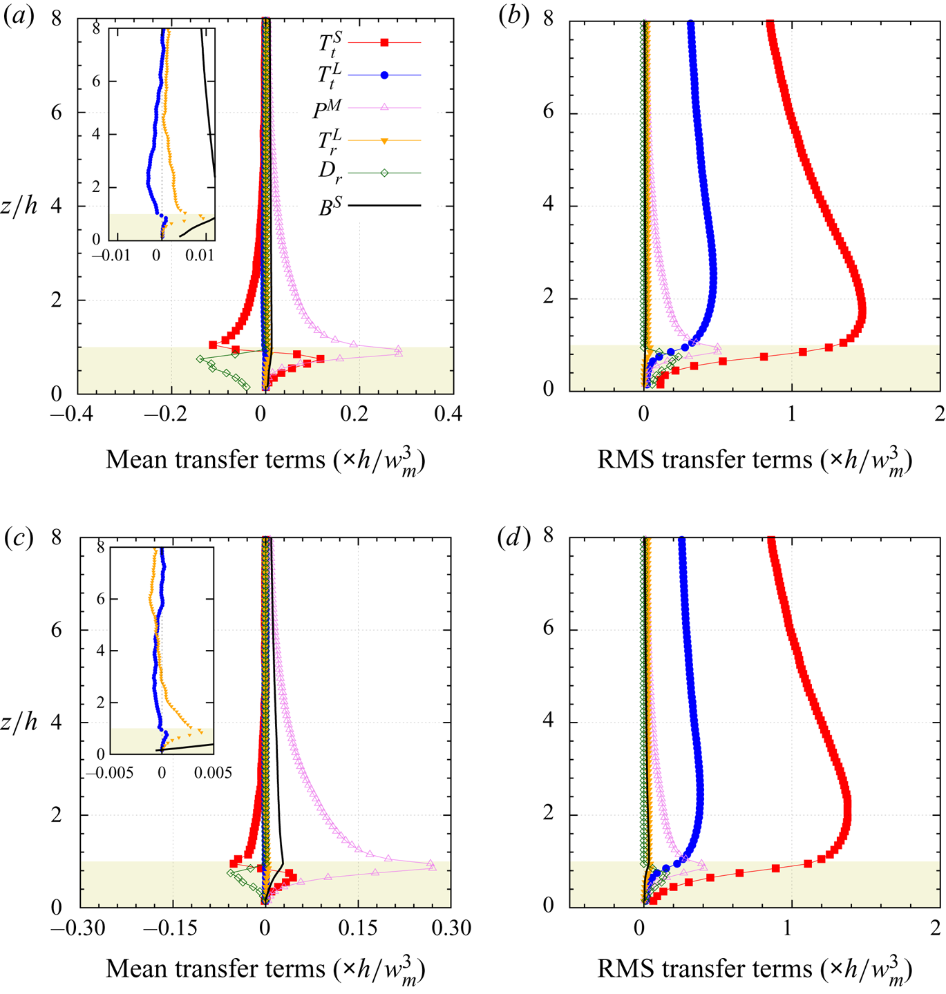
Figure 10. Wall-normal evolution of ( $a$,
$a$, $c$) the mean and
  $(b,\!d)$ standard deviation of the interscale transfer terms (
 $\blacksquare$, red)
  $T_t^S$, (
 $\bullet$, blue)
  $T_t^L$, (
 $\triangle$, pink)
  $P^M$, (
 $\blacktriangledown$, orange)
  $T_r^L$, (
 $\diamond$, green)
  $D_r$ and (solid black line)
  $B^S$ (as in table 2) for (
 $a$,
$a$, $b$) the small-scale TKE
  $(\xi ^S)^2$ and (
 $c$,
$c$, $d$) RSS
  $-u^Sw^S$ (WU case). Positive values indicate a gain for the small scales.
The primary findings regarding the transport of small-scale turbulent kinetic energy in the WU configuration can be summarized as follows (figure 10 $a$). As expected, the production term
  $P^M$ is always positive, confirming that the mean flow is a source term of TKE. The spatial transport term
  $T_t^S$ acts as a source term within the canopy (with a peak at the same height as the production term
  $P^M$), and a sink term just above the canopy. The small-scale component
  $({\boldsymbol{u}^S})$ transports its energy from above into the canopy. As
  ${\boldsymbol{u}^S}$ represents in this region the most energetic scales (figure 6), which is consistent with previous studies of TKE budgets within and above canopies which did not decompose each term by scale (Brunet et al. Reference Brunet, Finnigan and Raupach1994; Dwyer, Patton & Shaw Reference Dwyer, Patton and Shaw1997). The turbulent transport term
  $T_t^L$ of
  $(\xi ^S)^2$ by
  ${\boldsymbol{u}^L}$ is one order of magnitude smaller than the other terms, which agrees with the findings of Kawata & Alfredsson (Reference Kawata and Alfredsson2018) in the case of a plane Couette flow.
  $T_t^L$ is positive within the canopy, meaning that the large scales
  ${\boldsymbol{u}^L}$ transport small-scale energy into the canopy layers of the flow, and is negative above the canopy demonstrating that large-scale turbulence transports small-scale kinetic energy away from the roughness sublayer.
  $T_t^L$ becomes positive for
  $z/h>8$ with very low magnitude. The interscale energy transfer term
  $T_r^L$, which indicates nonlinear scale interaction (e.g. triadic interaction), is positive for all
  $z$ and peaks at canopy top. Intense mean wind speed shear in this region promotes small-scale TKE generation via the work of the small-scale Reynolds stresses against the spatial gradients of the large-scale velocity components. In the mean, TKE is transferred from large to small scales (classic forward scatter of energy), consistent with the concept of the energy cascade process. It can be noted that the sum of
  $T_r^L$ and
  $T_t^L$, which represents the global interaction between large and small scales, peaks (with a positive value) at canopy top and is dominated by the contribution of
  $T_r^L$ in this region. Within the canopy, the drag term
  $D_r$ acts as a sink of turbulent kinetic energy throughout the entire canopy (and is zero above) as expected. Finally, it is worth mentioning that the AM coefficient
  $AM(u^L,\xi ^S)$ involves the same quantity
  $u_i^Su_i^Su_j^L$ as the spatial transport term
  $T_t^L$, which suggests that
  $AM(u^L,\xi ^S)$ preferentially points to the influence of spatial transport rather than pure nonlinear interscale energy transfer. However, this last point only holds when the AM coefficient is based on the term
  $u_i^Su_i^Su_j^L$ (as in Basley et al. (Reference Basley, Perret and Mathis2018) or Blackman & Perret (Reference Blackman and Perret2016)) and not when defined using the low-pass-filtered envelope of the small scales calculated as the Hilbert transform of the small-scale signals, as in Mathis et al. (Reference Mathis, Hutchins and Marusic2009) or Salesky & Anderson (Reference Salesky and Anderson2018).
The standard deviations of these interaction terms controlling the transport of small-scale TKE are of a similar order of magnitude as their respective mean values or even greater by a factor of four to five for  $T_t^S$ and
  $T_t^L$ (figure 10
 $b$). In decreasing order of standard deviation, the five different transport terms rank as follows within the canopy:
  $T_t^S > T_t^L > P^M > D_r > T_r^L > B^S$. From an instantaneous or local point of view, intense events of both forward- and backscatter of energy exist, and are dominated by spatial transport, and then by interscale transfer
  $T_r^L$. The standard deviation of
  $T_t^L$ being larger than that of
  $T_r^L$ shows that instantaneous spatial transport dominates in the redistribution of energy.
Turning focus now to the small-scale RSS (figure 10 $c$), the main results are the following. Similar conclusions as for the small-scale TKE terms can be drawn concerning
  $T_t^S, P^M$ and
  $D_r$, which do not involve large-scale – small-scale interactions. The spatial transport term
  $T_t^L$ is positive just below
  $z/h=1$, negative for
  $1 < z/h < 6-7$ and positive (close to zero) above. Small-scale RSS is therefore transported away from the near-canopy region by
  ${\boldsymbol{u}^L}$. Positive values of the interscale transfer term
  $T_r^L$ for
  $z<3h$ (e.g. in the roughness sublayer) indicate forward interscale transfer (e.g. from
  ${\boldsymbol{u}^L}$ to
  ${\boldsymbol{u}^S}$), while above
  $z/h\simeq 3, T_r^L$ becomes negative indicating a backscatter mechanism with RSS transfer from
  ${\boldsymbol{u}^S}$ to
  ${\boldsymbol{u}^L}$, consistent with Kawata & Alfredsson (Reference Kawata and Alfredsson2018). Above
  $z/h\simeq 4$, the sum
  $T_t^L + T_r^L$ remains negative (not shown here), suggesting a net loss of small-scale Reynolds shear stress to the large scales. Finally, conclusions drawn on the standard deviation of all the terms from the analysis of the small-scale TKE remain valid for those of the RSS (figure 10
 $d$).
$d$).
3.6. Influence of stability
Atmospheric stability's influence on the wall-normal distribution of the AM coefficients between the large-scale velocity components  $u_i^L$ and the small-scale TKE
  $(\xi ^S)^2$ is shown in figure 11. The same trends as for the WU case are found for
  $AM(u^L,\xi ^S)$ and
  $AM(w^L,\xi ^S)$, for all the stability cases, namely positive (negative) values of
  $AM(u^L,\xi ^S)$ (
 $AM(w^L,\xi ^S)$) within the canopy and negative (positive) above. Atmospheric stability seems to influence more the wall-normal evolution of
  $AM(v^L,\xi ^S)$ with a sign change in
  $AM(v^L,\xi ^S)$ between the NN case and all other stability cases below
  $z/h=2$. This difference is attributed to the influence of the Coriolis forces on the spanwise component
  $v$ which decreases with increasing
  $-z_i/L$ and the fact that no coordinate rotation was performed to align the horizontal velocity component with the local mean wind. As found by Salesky & Anderson (Reference Salesky and Anderson2018), at any wall-normal location, the magnitude of
  $AM(u^L,\xi ^S)$ (and
  $AM(v^L,\xi ^S)$) decreases with increasing
  $-z_i/L$, even dropping to zero for
  $z/h > 8$ (or
  $z/z_i>0.16$) for the most unstable case (figure 11
 $a$). Regarding the influence of the large-scale wall-normal velocity component
  $w^L$ (figure 11
 $c$), the general trend is a reduction of the magnitude of
  $AM(w^L,\xi ^S)$ with increasing
  $-z_i/L$ but with non-zero values, indicating a persistent influence of the large-scale updraft on the canopy-scale turbulence. Nevertheless, our results demonstrate clear differences from Salesky & Anderson (Reference Salesky and Anderson2018) who found little influence of stability on
  $AM(w^L, \xi ^S)$ when interrogating turbulent flows interacting with parameterized roughness, which suggests a key influence of explicitly resolving processes produced by the inflection-point instability at canopy top. The mean transport terms of the small-scale TKE budget are analysed as a function of
  $-z_i/L$ (figure 12). As expected given the decrease of the imposed geostrophic wind with increasing
  $-z_i/L$, the production of small-scale TKE
  $P^M$ drops to zero with increasing
  $-z_i/L$. In the most unstable cases, the flow is no longer shear driven but buoyancy driven through the influence of the term
  $B^S$. This term, whose magnitude is almost independent of the atmospheric stability (with a peak value around
  $0.012h/w_m^3$ except for the FC case which peaks at
  $0.015h/w_m^3$), becomes the predominant source term of small-scale TKE with increasing
  $-z_i/L$. Spatial transport of small-scale energy by the large scales
  $T_t^L$ drops to zero with increasing
  $-z_i/L$ while spatial transport of small-scale energy by the small scales
  $T_t^S$ also decreases with
  $-z_i/L$ but stays non-zero in the roughness sublayer. The height of the (positive) peak of
  $T_t^S$ remains the same for all
  $-z_i/L$. The region of negative
  $T_t^S$ above the canopy extends to higher heights with increasing
  $-z_i/L$. It is therefore consistent with the existence of a mixing-layer region in which small-scale energy is transported by small scales from above the canopy into the canopy, with a wall-normal extent of a few times
  $h$. The interscale energy transfer term
  $T_r^L$ remains positive, consistent with the classic energy cascade process. Through drag, the canopy remains a sink term of kinetic energy (negative values of
  $D_r$) as expected. Decomposing the global drag term
  $D_r$ by scale (as in (2.19)) shows that the major contribution comes from the interaction between the small scales and the mean velocity field, followed by the interaction among small scales (not shown). Energy exchange via interaction between the large and small scales is two orders of magnitude smaller than the leading term, indicating that the influence of the large scales on the small scales through drag is negligible compared with that of mean shear. Finally, the conclusions associated with interrogating the standard deviation of the interaction terms from the WU case (§ 3.5) remain valid with increasing instability (not shown); a result indicating that no matter the stability regime, large and small scales interact instantaneously and predominantly through spatial transport. Regarding the transport of small-scale RSS (figure 13), all transport terms drop progressively to zero with increasing
  $-z_i/L$ while their standard deviations remain high and almost independent of the stability regime. In the FC case, the source term
  $B^S$ also becomes zero as the covariance
  $\langle \theta _v^S u^S \rangle$ (as well as
  $\langle \theta _v^S v^S\rangle$) drops to zero due to the isotropic character in the horizontal plane of the convection cells. To highlight the importance of the mean interscale transfer of TKE or RSS, the term
  $T_r^L$ is shown in figure 14 normalized by the production terms
  $P^M + B^S$. As mentioned above, all flow configurations show forward scatter of TKE from the large to the small scales with increasing relative magnitude with increasing
  $-z_i/L$ (figure 14
 $a$). It must be noted that as the influence of the mean shear decreases, a peak of
  $T_r^L/(P^M + B^S)$ appears at canopy top, reaching almost 60 % for the FC case. This indicates that as the mean shear production term vanishes, the large scales become a non-negligible source of TKE for the near-canopy structures. Except for the NN case, which shows an almost constant with height forward scatter of RSS (close to 2 %), backscatter of RSS exists for all other atmospheric stability cases above
  $z/h\simeq 2$ with an increasing relative importance with increasing
  $-z_i/L$ (figure 14
 $b$).
$b$).

Figure 11. The AM coefficients  $AM(u_i^L,\xi ^S)$ between the small-scale TKE
  $(\xi ^S)^2$ and the large-scale
  $(a)$ streamwise velocity component
  $u^L$,
  $(b)$ spanwise velocity component
  $v^L$ and
  $(c)$ wall-normal velocity component
  $w^L$, for each atmospheric stability cases listed in table 1.
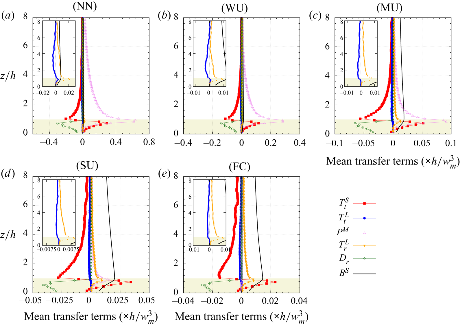
Figure 12. Wall-normal profiles of the mean interscale transfer terms ( $\blacksquare$, red)
  $T_t^S$, (
 $\bullet$, blue)
  $T_t^L$, (
 $\triangle$, pink)
  $P^M$, (
 $\blacktriangledown$, orange)
  $T_r^L$, (
 $\diamond$, green)
  $D_r$ and (black solid line)
  $B^S$ for the small-scale TKE
  $(\xi ^S)^2$, for all the atmospheric stability cases listed in table 1. Positive values indicate a gain for the small scales. Please note that the
  $x$-axis range changes between panels.
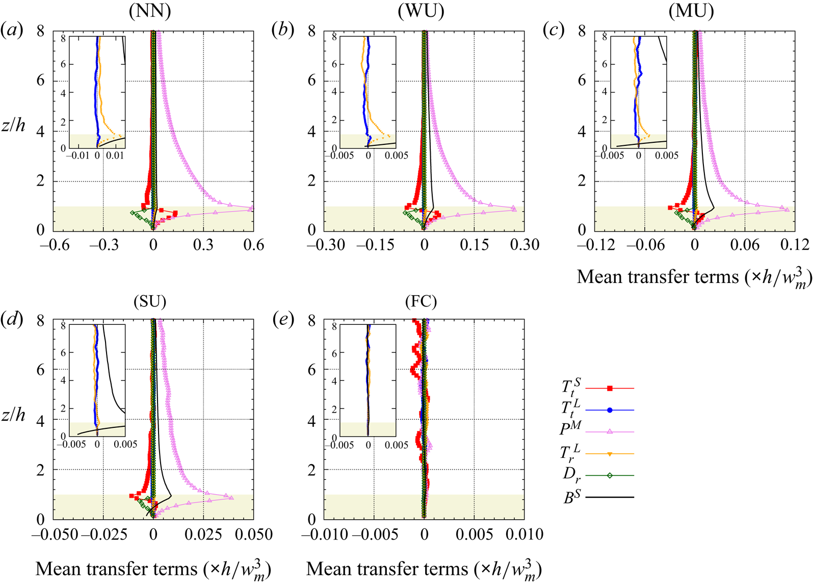
Figure 13. Wall-normal profiles of the mean interscale transfer terms ( $\blacksquare$, red)
  $T_t^S$, (
 $\bullet$, blue)
  $T_t^L$, (
 $\triangle$, pink)
  $P^M$, (
 $\blacktriangledown$, orange)
  $T_r^L$ and (
 $\diamond$, green)
  $D_r$ and (black solid line)
  $B^S$ for the small-scale RSS
  $-u^Sw^S$, for all the atmospheric stability cases listed in table 1. Positive values indicate a gain for the small scales. Please note that the
  $x$-axis range changes between panels.

Figure 14. Mean interscale transfer term  $T_r^L$ normalized by the sum of the shear and buoyancy production terms
  $P^M+B^S$ for
  $(a)$ small-scale TKE
  $(\xi ^S)^2$, and
  $(b)$ the small-scale RSS
  $-u^S w^S$, as a function of the wall-normal distance, for the five stability regimes. See corresponding text for the definition of each term.
This section's discussion clearly demonstrates atmospheric stability's influence on the vertical flow structure and subsequently the mechanisms controlling energy transport. Increasing instability ( $-z_i/L \rightarrow +\infty$) results in reduced mechanical turbulence production by reducing mean wind speed shear magnitudes in the lower regions of the flow. However, it has been shown (e.g. Patton et al. Reference Patton, Sullivan, Shaw, Finnigan and Weil2016; Salesky & Anderson Reference Salesky and Anderson2018) that increasing
  $-z_i/L$ and changing the stability regime from neutral to free convection drastically changes the instantaneous structure of the flow. The elongated roll structures visible in weakly unstable and near-neutral regime (figure 5) indeed transition to cellular convective structures with increasing
  $-z_i/L$ (not shown). Complementary to our analysis of the interscale transfer terms (see discussion surrounding figures 12 and 14), we now study the influence the evolution ABL-scale structure with increasing atmospheric instability (i.e. the evolution from rolls to cells) has on interscale energy transfer
  $T_r^L$ by interrogating stability's influence on contributions from subcomponent terms comprising
  $T_r^L$ that involve horizontal gradients of the large-scale velocity field. In the following,
  $T_{r,xy}^{u_i L}$ denotes the component
  $(G_3-I){\mathcal {L}}_{ix}^{L}({\delta u_i^L}/{\partial x}) + (G_3-I){\mathcal {L}}_{iy}^{L}({\delta u_i^L}/{\partial y})$ of
  $T_r^L$ (with no implicit summation over repeated index
  $i$ here). Here,
  $T_{r,xy}^L$ represents the contribution of the horizontal gradients of the three large-scale velocity components to
  $T_r^L$. The contribution of the vertical gradient of the LSM is represented by the difference
  $T_r^L - T_{r,xy}^{L}$. Wall-normal profiles of
  $T_r^L, T_{r,xy}^{u_i L}$ (with
  $i=1$, 2 or 3) and
  $T_{r,xy}^{L}$ are presented in figure 15.

Figure 15. Contribution of the terms involving horizontal gradients of the large-scale velocity field to the TKE interscale transfer term  $T_r^L$ as a function of the wall-normal distance, for the five stability regimes. See corresponding text for the definition of each term.
First, for any stability regime, the difference  $T_r^L - T_{r,xy}^{L}$ indicates that the terms involving the vertical gradient of the LSM are responsible for the forward scatter peak at canopy top (difference between the orange line,
  $T_r^L$ and the dark-green diamond (
 $\diamond$, green)
  $T_{r,xy}^L$) which is consistent with the classic turbulence kinetic energy production process, namely the work of small-scale shear stress against vertical gradient of large-scale velocity components. Above
  $z/h=2$, the horizontal gradients of the large-scale motion are major contributors to interscale energy transfer, with contribution from the different velocity components varying with
  $-z_i/L$. In particular, there is an increasing contribution of the vertical large-scale velocity component
  $w^L$ to interscale transfer with increasing
  $-z_i/L$. The contribution of the horizontal velocity components (
 $u^L$ and
  $v^L$) peaks at
  $z/h \simeq 2$ or a bit lower for the free-convective case while the influence of
  $w^L$ starts higher if present. For all stability cases, the global trend is the following: there is a major contribution of the horizontal gradients of (
 $\triangle$, pink)
  $u^L$, then (
 $\blacktriangledown$, red)
  $v^L$ and then (
 $\bullet$, blue)
  $w^L$, the latter being close to zero for weak convective regimes. The influence of
  $w^L$ indeed becomes significant and predominant only for the two most unstable cases and impacts the region
  $z/h>2$, consistent with the analysis of the AM coefficient
  $AM(w^L,\xi ^S)$ as a function of
  $-z_i/L$.
4. Conclusion
Based on high-resolution LES data of an ABL developing over a vegetation canopy, the interaction between the most energetic large-scale structures existing in the ABL and the small scales originating from the near-canopy region has been investigated. The main findings are the following:
(i) In spite of the presence of the vegetation canopy in the near-wall region, the AM mechanism of the small scales by the most energetic structures of the ABL is found to exist and involve all three velocity components of both large and small scales, in agreement with prior studies conducted in laboratory flows over smooth (Mathis et al. Reference Mathis, Hutchins and Marusic2009; Bernardini & Pirozzoli Reference Bernardini and Pirozzoli2011; Jacobi & McKeon Reference Jacobi and McKeon2013; Talluru et al. Reference Talluru, Baidya, Hutchins and Marusic2014) or rough walls (Nadeem et al. Reference Nadeem, Lee, Lee and Sung2015; Anderson Reference Anderson2016; Blackman & Perret Reference Blackman and Perret2016; Squire et al. Reference Squire, Morill-Winter, Hutchins, Schultz, Klewicki and Marusic2016; Pathikonda & Christensen Reference Pathikonda and Christensen2017; Basley et al. Reference Basley, Perret and Mathis2018) and ABL flows (Lemone Reference Lemone1976; Salesky & Anderson Reference Salesky and Anderson2018; Liu, Wang & Zheng Reference Liu, Wang and Zheng2019). This influence exists also within the canopy, with AM coefficients peaking just below canopy top.
(ii) Through analysis of the scale-decomposed budget equation of the small-scale TKE, this link has been confirmed and quantified. In particular, it has been shown that in the mean, there exists a net transfer of energy from large to small scales while the large scales induce an upward spatial transport of energy from the near-canopy top to the region above. However, within the canopy and broader roughness sublayer, the magnitude of the net exchange between the large- and small-scale structures is weak (one order of magnitude smaller) relative to the other transport terms such as energy production by the mean flow, drag influence within the canopy or spatial transport of small-scale energy by the small scales themselves.
The interscale energy transfer found above the canopy in the ABL agrees well with the findings of Lemone (Reference Lemone1976) or Kawata & Alfredsson (Reference Kawata and Alfredsson2018) in flows over smooth surfaces.
The turbulent transport and interscale transfer terms of the energy budget equations are strongly tied to the classically investigated AM coefficients (see (3.1)) because they are based on the same third-order statistics.
However, direct deduction of AM coefficients from the turbulent transport and interscale transfer terms is not straightforward as the AM coefficients depend on the wall-normal evolution of the variances of both the large-scale envelope of the small scales and the large scales (used for normalization) while the constituents of the budget equation involve spatial gradients of third-order moments.
(iii) Despite the relatively small importance of the scale interaction in the net transfer of energy, analysis of the standard deviation of the transport terms demonstrates intense forward- and backscatter of energy. This finding supports the Mizuno (Reference Mizuno2016) conclusion that individual instantaneous events sustaining the energy spectra might be cancelled by others and therefore hidden when analysing bulk statistics.
This finding, along with the conclusion drawn by Patton et al. (Reference Patton, Sullivan, Shaw, Finnigan and Weil2016) when analysing the same data as in the present study, about the significant improvement of the skewness profiles when accounting for ABL-scale structures in LES of atmospheric flows above and within a vegetation canopy must also relate to the conclusions of Brasseur & Wei (Reference Brasseur and Wei1994) and Yeung, Brasseur & Wang (Reference Yeung, Brasseur and Wang1995) about interscale dynamics. These studies indeed demonstrated that triadic interactions between distant scales (i.e. when the ratio between scales is greater than 15–20, Brasseur & Wei Reference Brasseur and Wei1994) induce weak energy transfers and are embedded in energy cascading interactions among scales of similar magnitude but create phase correlation and anisotropy at the small scales that shows in third-order moments.
(iv) Analysis of the budget equation of the small-scale RSS shows that, in the near-canopy region, large scales are a source of small-scale RSS through interscale transfer while those same large-scales act as a sink through spatial transport. These two mechanisms switch roles above the roughness sublayer. This combination can be interpreted as a feedback mechanism from the small to the large scales, as found by Kawata & Alfredsson (Reference Kawata and Alfredsson2018) in plane Couette flow. However, similar to kinetic energy, the magnitude of these terms remains small relative to the production, drag and other spatial transport terms. As for kinetic energy, the standard deviation of these scale-interaction terms is high compared with their mean value, indicating the occurrence of strong instantaneous forward- and backscatter exchange of RSS.
(v) Canopy drag constitutes a net sink term for both energy and RSS. However, the standard deviation of the drag term in the budget equation being twice its average value, drag also creates strong instantaneous forward- and backscatter. Compared with the mean flow–small-scale flow interaction, the contribution of the scale interaction to the net drag effect is weak.
(vi) Conclusions (i) through (v) remain valid with increasing
$-z_i/L$. However, the analysis of the AM shows that, consistent with Salesky & Anderson (Reference Salesky and Anderson2018), the vertical LSM $w^L$ plays an increasingly important role in the interscale transfer when buoyancy effects increase and the flow switches from being shear driven to being buoyancy driven.


Thus, even if AM coefficients show significant levels (up to 0.75, depending on the atmospheric stability), the average influence of the large ABL scales on the smaller canopy scales is weak, with the corresponding transfer terms being an order of magnitude smaller than production by the mean flow or buoyancy effects. However, even if small, the present findings support the existence of closed-loop pathway between large and small scales, with strong instantaneous forward and backward exchange of both kinetic energy and RSS. The recent findings from Hwang & Cossu (Reference Hwang and Cossu2010) showing that large-scale structures in the outer region are self-sustaining and mainly a consequence of the structure of the mean flow profile but also the fact that mean shear (or buoyancy) is the key contributor in near-wall turbulence generation raises the question of the role of the instantaneous scale interaction in the dynamics of the flow. The present conclusions combined with those of Patton et al. (Reference Patton, Sullivan, Shaw, Finnigan and Weil2016) about the importance of including ABL-scale eddies in LES of the ABL over vegetation canopy to more accurately reproduce the skewness profiles, along the line of the findings of Brasseur & Wei (Reference Brasseur and Wei1994) draw the attention to the dynamical role of the scale interaction and call for further investigation.
Finally, the modulation of small-scale turbulence by larger scales discussed in this paper clearly demonstrates the importance of large-scale (ABL-scale) turbulence on velocity skewness and the instantaneous dynamics of smaller-scale turbulence within and above vegetation canopies. Therefore, while previous studies of atmospheric canopy turbulence utilizing limited-height domains have provided substantial insight into the mechanics of canopy-scale turbulence (e.g. Shaw & Schumann (Reference Shaw and Schumann1992), among many others), those simulations are likely producing accurate first- and second-order statistics for reasons that are distinct from those controlling canopy turbulence observed in field measurements. This analysis also demonstrates that the modulation of the small-scale structures by the large scales leads to the local enhancement/reduction of small-scale activity in a canopy's vicinity which introduces spatially heterogeneous flow characteristics at the scale of the ABL-scale structures. This effect averages out in flows over horizontally homogeneous terrain if averaging strategies incorporate ABL scales, however, land surface heterogeneity (e.g. orography, land use) could promote and positionally lock ABL-scale motions to a particular spatial location thereby ensuring the influence would persist.
Acknowledgements
We also acknowledge high-performance computing support from: (i) Yellowstone (ark:/85065/d7wd3xhc) provided by NCAR's Computational and Information Systems Laboratory, sponsored by the National Science Foundation, and (ii) the National Energy Research Scientific Computing Center (NERSC), a U.S. Department of Energy Office of Science User Facility operated under Contract No. DE-AC02-05CH11231. The authors also acknowledge comments and suggestions from two anonymous reviewers that improved the manuscript.
Funding
This material is based upon work supported by the National Center for Atmospheric Research, which is a major facility sponsored by the National Science Foundation under Cooperative Agreement No. 1852977. E.G.P. acknowledges supplemental support from NCAR's Geophysical Turbulence Program. L.P. acknowledges the financial support of Ecole Centrale de Nantes, the LHEEA laboratory, UMR CNRS 6598 and IRSTV, FR CNRS 2488, during his sabbatical leave at the National Center for Atmospheric Research.
Declaration of interests
The authors report no conflict of interest.
Appendix A. Scale-decomposed momentum transport equations using the multi-level filtering approach
A.1. Momentum transport equations in index form
Using index notation, the momentum transport equation (2.15) reads
 \begin{align} \frac{\partial \bar{u}_i^{(n)}}{\partial t} + \bar{u}_j^{(n)} \frac{\partial \bar{u}_i^{(n)}}{\partial x_j} &={-} f \epsilon_{ijl} \hat{k}_j(\bar{u}_l^{(n)} - \bar{U}_{gl}^{(n)}) - \frac{\partial \bar{\rm \pi}^{(n)}}{\partial x_i} + \beta (\bar{\theta}_v^{(n)}\delta_i^3 - \bar{\theta}_{v_0}^{(n)}) \nonumber\\ &\quad - \frac{\partial T_{ij}^{(n)}}{\partial x_j} + \bar{{F}}_{d_i}^{(n)}, \end{align}
or, equivalently,
 \begin{equation} \frac{\partial \bar{u}_i^{(n)}}{\partial t} + \bar{u}_j^{(n)} \frac{\partial \bar{u}_i^{(n)}}{\partial x_j} = \bar{L}_i^{(n)} - \frac{\partial T_{ij}^{(n)}}{\partial x_j} + \bar{{F}}_{d_i}^{(n)},\end{equation}
with
 \begin{equation} T_{ij}^{(n)} =\overline{u_i u_j}^{(n)} - \bar{u}_i^{(n)} \bar{u}_j^{(n)}. \end{equation}
Here,  $\bar {L}_i^{(n)}$ is given by (2.14) while the detail of
  $\bar {F}_{d_i}^{(n)}$ can be found in Appendix A.3.
A.2. Calculation of $(\boldsymbol{{T}}^{(n)} -\boldsymbol{{T}}^{(n+1)})$

Using the multi-level Germano identity (Sagaut et al. Reference Sagaut, Deck and Terracol2013, § 4.2.1.2), SFS tensors  ${\boldsymbol{T}}^{(n)}$ and
  ${\boldsymbol{T}}^{(n)}$ with
  $m< n$ between two different filtering levels
  $n$ and
  $m$, respectively, can be related by
 \begin{equation} T_{ij}^{(n)} = {\mathcal{L}}_{ij}^{(n)} + \sum_{k=m+1,n-1} {\mathcal{G}}_{k+1}^n {\mathcal{L}}_{ij}^{(k)} + {\mathcal{G}}_{m+1}^n {T}_{ij}^{(m)}, \end{equation}
with
 \begin{gather} T_{ij}^{(n)} =\overline{u_i u_j}^{(n)} - \overline{u_i}^{(n)} \overline{u_j}^{(n)}, \end{gather}
 \begin{gather}T_{ij}^{(n+1)} = G_{n+1} \star T_{ij}^{(n)}+{\mathcal{L}}_{ij}^{(n+1)}, \end{gather}
and
 \begin{equation} {\mathcal{L}}_{ij}^{(n+1)} =G_{n+1} \star (\bar{u}_i^{(n)}\bar{u}_j^{(n)} ) -\bar{u}_i^{(n+1)}\bar{u}_j^{(n+1)}. \end{equation}
As depicted in figure 2, the different terms in the above equations can be interpreted as follows:  ${\mathcal {L}}_{ij}^{(n)}$ represents the influence of ‘sub-level scales’
  $\delta {\boldsymbol{u}}^{(n-1)}$ at the
  $n$th level contributing to
  $\bar {{\boldsymbol{u}}}^{(n)}$ (e.g. interaction between
  $\bar {{\boldsymbol{u}}}^{(n)}$ and
  $\delta {\boldsymbol{u}}^{(n-1)}$);
  ${\mathcal {G}}_{k+1}^{(n)}{\mathcal {L}}_{ij}^{(k)}$ bears the influence of the ‘sub-level scales’
  $\delta {\boldsymbol{u}}^{(k-1)}$ at the
  $k$th level contributing to
  $\bar {{\boldsymbol{u}}}^{(n)}$ (e.g. interaction between
  $\bar {{\boldsymbol{u}}}^{(k)}$ and
  $\delta {\boldsymbol{u}}^{(k-1)}$ filtered at level
  $n$);
$n$);  ${\mathcal {G}}_{m+1}^{(n)}T_{ij}^{(m)}$ represents the influence of the ‘sub-level scales’
  $\delta {\boldsymbol{u}}^{(m)}+{\boldsymbol{u}}{^{\prime \prime }}$ at the
  $m$th level contributing to
  $\bar {{\boldsymbol{u}}}^{(n)}$ (e.g. interaction between
  $\bar {{\boldsymbol{u}}}^{(m+1)}$ and both the resolved band-pass-filtered velocity
  $\delta {\boldsymbol{u}}^{(m)}$ and the SFS field
  ${\boldsymbol{u}}^{\prime \prime }$ filtered at level
  $n$).
$n$).
With the above, the term  $({\boldsymbol{T}}^{(n)} -{\boldsymbol{T}}^{(n+1)})$ therefore reads
 \begin{align} T_{ij}^{(n+1)} & = {\mathcal{L}}_{ij}^{(n+1)} + \sum_{k=m+1,n+1-1} {\mathcal{G}}_{k+1}^{n+1} {\mathcal{L}}_{ij}^{(k)} + {\mathcal{G}}_{m+1}^{n+1} {T}_{ij}^{(m)} \nonumber\\ & = {\mathcal{L}}_{ij}^{(n+1)} + \sum_{k=m+1,n-1} {\mathcal{G}}_{k+1}^{n+1} {\mathcal{L}}_{ij}^{(k)} + {\mathcal{G}}_{n+1-1+1}^{n+1} {\mathcal{L}}_{ij}^{(n+1-1)} + {\mathcal{G}}_{m+1}^{n+1} {T}_{ij}^{(m)} \nonumber\\ & = {\mathcal{L}}_{ij}^{(n+1)} + \sum_{k=m+1,n-1} {\mathcal{G}}_{k+1}^{n+1} {\mathcal{L}}_{ij}^{(k)} + {\mathcal{G}}_{n+1}^{n+1} {\mathcal{L}}_{ij}^{(n)} + {\mathcal{G}}_{m+1}^{n+1} {T}_{ij}^{(m)} \nonumber\\ & = {\mathcal{L}}_{ij}^{(n+1)} + \sum_{k=m+1,n-1} {\mathcal{G}}_{k+1}^{n+1} {\mathcal{L}}_{ij}^{(k)} + G_{n+1} {\mathcal{L}}_{ij}^{(n)} + {\mathcal{G}}_{m+1}^{n+1} {T}_{ij}^{(m)}, \end{align}
with
 \begin{equation} T_{ij}^{(n)} = {\mathcal{L}}_{ij}^{(n)} + \sum_{k=m+1,n-1} {\mathcal{G}}_{k+1}^n {\mathcal{L}}_{ij}^{(k)} + {\mathcal{G}}_{m+1}^n {T}_{ij}^{(m)}. \end{equation}
Hence
 \begin{align} T_{ij}^{(n+1)}-T_{ij}^{(n)} &= {\mathcal{L}}_{ij}^{(n+1)} + \sum_{k=m+1,n-1} ({\mathcal{G}}_{k+1}^{n+1}-{\mathcal{G}}_{k+1}^{n} ) {\mathcal{L}}_{ij}^{(k)} \nonumber\\ &\quad + (G_{n+1}-I ) {\mathcal{L}}_{ij}^{(n)} + (G_{n+1}-I ){\mathcal{G}}_{m+1}^{n} {T}_{ij}^{(m)}. \end{align}
A.3. Calculation of the drag term $( \bar {{\boldsymbol{F}}}_d^{(n)}- \bar {{\boldsymbol{F}}}_d^{(n+1)} )$

In the general case, the drag force created by the presence of the canopy is modelled as (Shaw & Patton Reference Shaw and Patton2003)
 \begin{equation} {\boldsymbol{F}}_d ={-}(c_d+c_{sf})a v_w {\boldsymbol{u}}, \end{equation}
where  $c_d$ is the form drag coefficient,
  $c_{sf}$ is the viscous drag coefficient (Reynolds number dependent),
  $a$ is a one-sided frontal plant area density and
  $v_w$ is the wind speed magnitude with
  $v_w^2=|{{\boldsymbol{u}}}|^2=u_i u_i = u_1^2+u_2^2+u_3^2$. Following Shaw & Patton (Reference Shaw and Patton2003), the viscous canopy-drag term is assumed negligible (
 $c_{sf}=0$) compared with canopy form drag and depends only on the LES resolved scales
  $\bar {{\boldsymbol{u}}}$ (Patton et al. Reference Patton, Sullivan, Shaw, Finnigan and Weil2016). Wakes shed in the lee of canopy elements are presumed small enough so that they directly dissipate to heat hence the term
  $F_\epsilon$ in the LES transport equation for SFS TKE
  $e$ (which solely represents the work performed by SFS motions against canopy drag) (Patton et al. Reference Patton, Sullivan, Shaw, Finnigan and Weil2016). The drag force is therefore parametrized as (Shaw & Schumann Reference Shaw and Schumann1992)
 \begin{equation} {\boldsymbol{F}}_d ={-}c_d a \overline{{v_w}} \bar{{\boldsymbol{u}}}, \end{equation}
where  $\overline {{v_w}}=|\bar {{\boldsymbol{u}}}|=\sqrt {\overline {u_i} \overline {u_i}}$ is the local velocity magnitude. The scalar
  $\overline {{v_w}}$ depends solely on the resolved velocity field and can therefore be computed directly.
Using the multi-level filtering formalism, neglecting the viscous canopy drag ( $c_{sf}=0$) and using the parametrization from Shaw & Schumann (Reference Shaw and Schumann1992) (see (A12)), (A11) reads
 \begin{align} {\boldsymbol{F}}_d & = \bar{{\boldsymbol{F}}}_d^{(1)} \nonumber\\ & ={-}c_d a \overline{v_w {\boldsymbol{u}}}^{(1)}\nonumber\\ & ={-}c_d a \overline{v_w}^{(1)}\bar{{\boldsymbol{u}}}^{(1)} + \boldsymbol{d}^{(1)}\nonumber\\ & = \boldsymbol{ D}^{(1)}+ \boldsymbol{ d}^{(1)}, \end{align}
where  $\boldsymbol {d}^{(1)}=0$ represents the contribution of the SFS field to the drag (which is zero in the present case, at the lowest level of filtering, Shaw & Schumann Reference Shaw and Schumann1992). This contribution can be viewed as being similar to a SFS tensor
  $\boldsymbol {d}^{(1)}=-c_d a (\overline {v_w{\boldsymbol u}}^{(1)}-\overline {v_w}^{(1)}\bar {{\boldsymbol u}}^{(1)})$. At level
  $n$, the drag force can be decomposed into
 \begin{equation} \bar{{\boldsymbol F}}_d^{(n)} = \boldsymbol{D}^{(n)}+ \boldsymbol{d}^{(n)}, \end{equation}
with  $\boldsymbol {D}^{(n)}=-c_d a \overline {v_w}^{(n)} \bar {{\boldsymbol u}}^{(n)}$ and
  $\boldsymbol {d}^{(n)}$ (for
  $m< n$) defined as
 \begin{equation} {d}_i^{(n)} = {\mathcal{D}}_i^{(n)} + \sum_{k=m+1,n-1} {\mathcal{G}}_{k+1}^n {\mathcal{D}}_i^{(k)}+ {\mathcal{G}}_{m+1}^n d_i^{(m)}, \end{equation}
with  $\boldsymbol {d}^{(1)}=0$ and (similarly to
  ${\mathcal {L}}_{ij}^{(n)}$)
 \begin{equation} {\mathcal{D}}_i^{(n+1)}={-}c_d a [ G_{n+1} (\overline{v_w}^{(n)}\bar{u}_i^{(n)} )- \overline{v_w}^{(n+1)}\bar{u}_i^{(n+1)}]. \end{equation}
If  $m=1$ and
  $n=2$,
 \begin{align} d_i^{(2)} & = {\mathcal{D}}_i^{(2)} + G_2 d_i^{(1)} = {\mathcal{D}}_i^{(2)}\nonumber\\ & ={-}c_d a [G_2 (\overline{v_w}^{(1)}\bar{u}_i^{(1)} )- \overline{v_w}^{(2)}\bar{u}_i^{(2)}]. \end{align}
If  $m=1$ and
  $n=3$,
 \begin{align} d_i^{(3)} & = {\mathcal{D}}_i^{(3)}+ G_3{\mathcal{D}}_i^{(2)}+G_3\star G_2 d_i^{(1)} \nonumber\\ &= {\mathcal{D}}_i^{(3)}+ G_3{\mathcal{D}}_i^{(2)}. \end{align}
Thus, as before, in the case of a four-level decomposition, with  $m=1$ and
  $n=2$,
 \begin{align} d_i^{(n+1)}-d_i^{(n)} &= d_i^{(3)}-d_i^{(2)} \nonumber\\ & = {\mathcal{D}}_i^{(3)} + (G_3 - I ){\mathcal{D}}_i^{(2)} \end{align}
(because  $\boldsymbol {d}^{(1)}=0$). Therefore,
  ${\mathcal {D}}_{i}^{(3)}$ can be interpreted as the contribution of
  $\delta {\boldsymbol u}^{(2)}={\boldsymbol u}^{L}$ to the drag at level 3 or
  ${\boldsymbol u}^{M}, (G_3 - I ){\mathcal {D}}_{i}^{(2)}$ represents the contribution of the band-pass-filtered velocity
  $\delta {\boldsymbol u}^{(1)}={\boldsymbol u}^{S}$ to the drag at level of the band-pass filtered velocity
  $\delta {\boldsymbol u}^{(2)}={\boldsymbol u}^{L}$. In addition, with the present hypothesis, the contribution of the SFS scales to the drag is zero.
Appendix B. Transport equation of $\delta$KE$^{(n)}$ the kinetic energy of $\delta {\boldsymbol u}^{(n)}$


B.1. Equation derivation
The transport equation of the momentum associated with the band-pass filtered velocity  $\delta {\boldsymbol u}^{(n)}=\bar {\boldsymbol u}^{(n)}-\bar {\boldsymbol u}^{(n+1)}$ is obtained by subtracting the transport equation for
  $\bar {\boldsymbol u}^{(n+1)}$ from that for
  $\bar {\boldsymbol u}^{(n)}$. With the above drag decomposition, it reads
 \begin{align} & \frac{\partial {\delta{\boldsymbol u}}^{(n)}}{\partial t} + \boldsymbol{\nabla} \boldsymbol{\cdot} ( {\delta{\boldsymbol u}}^{(n)} \otimes {\delta{\boldsymbol u}}^{(n)} +{\delta{\boldsymbol u}}^{(n)} \otimes \bar{{\boldsymbol u}}^{(n+1)} + \bar{{\boldsymbol u}}^{(n+1)}\otimes {\delta{\boldsymbol u}}^{(n)})\nonumber\\ &\quad = \delta {\boldsymbol L}^{(n)} -\boldsymbol{\nabla} \boldsymbol{\cdot} ( {\boldsymbol T}^{(n)} -{\boldsymbol T}^{(n+1)} ) + ( \boldsymbol{D}^{(n)}- \boldsymbol{D}^{(n+1)}) + (\boldsymbol{d}^{(n)}-\boldsymbol{d}^{(n+1)} ), \end{align}
or, with index notation (from (2.10))
 \begin{align} & \frac{\partial {\delta u}_i^{(n)}}{\partial t} +\frac{\partial}{\partial x_j} ({\delta u}_i^{(n)} {\delta u}_j^{(n)} +{\delta u}_i^{(n)} {\bar{u}}_j^{(n+1)} + {\bar{u}}_i^{(n+1)} {\delta u}_j^{(n)}) \nonumber\\ &\quad = \delta {L}_i^{(n)} -\frac{\partial}{\partial x_j} ( {T}_{ij}^{(n)} -{T}_{ij}^{(n+1)} ) + ( {{D}}_{i}^{(n)}- {{D}}_{i}^{(n+1)}) + ({d}_{i}^{(n)}-{d}_{i}^{(n+1)} ). \end{align}
In order to derive the transport equation of the kinetic energy of  $\delta {\boldsymbol u}^{(n)}$, the above equation is written for the component
  $\delta {u}_i^{(n)}$, multiplied by
  $\delta {u}_i^{(n)}$, followed by a contraction over the repeated index
  $i$
$i$
 \begin{align}
& \frac{1}{2}\frac{\partial}{\partial t} ({\delta
u}_i^{(n)}{\delta u}_i^{(n)}) +\frac{\partial}{\partial
x_j} \left(\frac{1}{2}{\delta u}_i^{(n)}{\delta u}_i^{(n)}
{\delta u}_j^{(n)} +\frac{1}{2}{\delta u}_i^{(n)}{\delta
u}_i^{(n)} {\bar{u}}_j^{(n+1)}\right)\nonumber\\
& \hspace{5.7pc} +{\delta u}_i^{(n)}\frac{\partial}{\partial x_j}({\bar{u}}_i^{(n+1)} {\delta u}_j^{(n)})\nonumber\\
& \quad = \delta {L}_i^{(n)}{\delta
u}_i^{(n)}+( {T}_{ij}^{(n)} -{T}_{ij}^{(n+1)} )
\frac{\partial {\delta{u}}_i^{(n)}}{\partial x_j}
-\frac{\partial}{\partial x_j} ( ({T}_{ij}^{(n)}
-{T}_{ij}^{(n+1)}){\delta u}_i^{(n)} )\nonumber\\ & \qquad
+ ( {{D}}_{i}^{(n)}- {{D}}_{i}^{(n+1)}){\delta u}_i^{(n)} +
({d}_{i}^{(n)}-{d}_{i}^{(n+1)} ){\delta u}_i^{(n)}.
\end{align}
\begin{align}
& \frac{1}{2}\frac{\partial}{\partial t} ({\delta
u}_i^{(n)}{\delta u}_i^{(n)}) +\frac{\partial}{\partial
x_j} \left(\frac{1}{2}{\delta u}_i^{(n)}{\delta u}_i^{(n)}
{\delta u}_j^{(n)} +\frac{1}{2}{\delta u}_i^{(n)}{\delta
u}_i^{(n)} {\bar{u}}_j^{(n+1)}\right)\nonumber\\
& \hspace{5.7pc} +{\delta u}_i^{(n)}\frac{\partial}{\partial x_j}({\bar{u}}_i^{(n+1)} {\delta u}_j^{(n)})\nonumber\\
& \quad = \delta {L}_i^{(n)}{\delta
u}_i^{(n)}+( {T}_{ij}^{(n)} -{T}_{ij}^{(n+1)} )
\frac{\partial {\delta{u}}_i^{(n)}}{\partial x_j}
-\frac{\partial}{\partial x_j} ( ({T}_{ij}^{(n)}
-{T}_{ij}^{(n+1)}){\delta u}_i^{(n)} )\nonumber\\ & \qquad
+ ( {{D}}_{i}^{(n)}- {{D}}_{i}^{(n+1)}){\delta u}_i^{(n)} +
({d}_{i}^{(n)}-{d}_{i}^{(n+1)} ){\delta u}_i^{(n)}.
\end{align}
Using the fact that  ${\bar {u}}_i^{(n)}={\bar {u}}_i^{(n+1)}+\delta {u}_i^{(n)}$ and
  ${\overline {v_w}}^{(n)}={\overline {v_w}}^{(n+1)}+\delta {v_w}^{(n)}$, the drag term becomes
 \begin{align} & {{D}}_{i}^{(n)} -{{D}}_{i}^{(n+1)} ={-}a c_d [{\overline{v_w}}^{(n)}{\bar{u}}_i^{(n)} -{\overline{v_w}}^{(n+1)}{\bar{u}}_i^{(n+1)}]\nonumber\\ &\quad ={-}a c_d [ {\overline{v_w}}^{(n+1)}{\bar{u}}_i^{(n+1)} +\delta{v_w}^{(n)}{\bar{u}}_i^{(n+1)} +{\overline{v_w}}^{(n+1)}{\delta u}_i^{(n)}\nonumber\\ &\qquad +\delta{v_w}^{(n)}{\delta{u}}_i^{(n)} -{\overline{v_w}}^{(n+1)}{\bar{u}}_i^{(n+1)}], \end{align}
thus
 \begin{equation} {{D}}_{i}^{(n)} -{{D}}_{i}^{(n+1)} ={-}a c_d [ \delta{v_w}^{(n)}{\delta{u}}_i^{(n)} +\delta{v_w}^{(n)}{\bar{u}}_i^{(n+1)} +{\overline{v_w}}^{(n+1)}{\delta u}_i^{(n)} ]. \end{equation}
The transport equation of the kinetic energy of  $\delta {\boldsymbol u}^{(n)}$ reads
 \begin{align}
\frac{\partial}{\partial t} \left(\frac{1}{2}{\delta u}_i^{(n)}{\delta u}_i^{(n)}\right)
& ={-}\frac{\partial}{\partial x_j} \left(\frac{1}{2}{\delta u}_i^{(n)}{\delta u}_i^{(n)}
{\delta u}_j^{(n)} +\frac{1}{2}{\delta u}_i^{(n)}{\delta u}_i^{(n)} {\bar{u}}_j^{(n+1)}\right) \nonumber\\
& \quad-{\delta u}_i^{(n)}\frac{\partial}{{\partial x_j}}({\bar{u}}_i^{(n+1)}{\delta u}_j^{(n)}) \nonumber\\
& \quad + \delta {L}_i^{(n)}{\delta u}_i^{(n)} +( {T}_{ij}^{(n)} -{T}_{ij}^{(n+1)} )
\frac{\partial {\delta u}_i^{(n)}}{\partial x_j} \nonumber\\
&\quad -\frac{\partial}{\partial x_j} ( ({T}_{ij}^{(n)}
-{T}_{ij}^{(n+1)}){\delta u}_i^{(n)} )\nonumber\\ & \quad -
a c_d ( \delta{v_w}^{(n)}{\delta{u}}_i^{(n)}{\delta
u}_i^{(n)} +\delta{v_w}^{(n)}{\delta
u}_i^{(n)}{\bar{u}}_i^{(n+1)}
+{\overline{v_w}}^{(n+1)}{\delta u}_i^{(n)}{\delta
u}_i^{(n)}) \nonumber\\ &\quad +
({d}_{i}^{(n)}-{d}_{i}^{(n+1)} ){\delta u}_i^{(n)} .
\end{align}
\begin{align}
\frac{\partial}{\partial t} \left(\frac{1}{2}{\delta u}_i^{(n)}{\delta u}_i^{(n)}\right)
& ={-}\frac{\partial}{\partial x_j} \left(\frac{1}{2}{\delta u}_i^{(n)}{\delta u}_i^{(n)}
{\delta u}_j^{(n)} +\frac{1}{2}{\delta u}_i^{(n)}{\delta u}_i^{(n)} {\bar{u}}_j^{(n+1)}\right) \nonumber\\
& \quad-{\delta u}_i^{(n)}\frac{\partial}{{\partial x_j}}({\bar{u}}_i^{(n+1)}{\delta u}_j^{(n)}) \nonumber\\
& \quad + \delta {L}_i^{(n)}{\delta u}_i^{(n)} +( {T}_{ij}^{(n)} -{T}_{ij}^{(n+1)} )
\frac{\partial {\delta u}_i^{(n)}}{\partial x_j} \nonumber\\
&\quad -\frac{\partial}{\partial x_j} ( ({T}_{ij}^{(n)}
-{T}_{ij}^{(n+1)}){\delta u}_i^{(n)} )\nonumber\\ & \quad -
a c_d ( \delta{v_w}^{(n)}{\delta{u}}_i^{(n)}{\delta
u}_i^{(n)} +\delta{v_w}^{(n)}{\delta
u}_i^{(n)}{\bar{u}}_i^{(n+1)}
+{\overline{v_w}}^{(n+1)}{\delta u}_i^{(n)}{\delta
u}_i^{(n)}) \nonumber\\ &\quad +
({d}_{i}^{(n)}-{d}_{i}^{(n+1)} ){\delta u}_i^{(n)} .
\end{align}
Note that  $\overline {v_w}^{(n)} >0, \delta v_w^{(n)}=\overline {|{\boldsymbol u}|}^{(n)}-\overline {|{\boldsymbol u}|}^{(n)+1} >0$ and
  $a c_d > 0$. Hence, in the last before drag term (on the right-hand side), the first and last terms are strictly negative, e.g. dissipative, while the sign second one (
 $\delta {v_w}^{(n)}{\delta u}_i^{(n)}{\bar {u}}_i^{(n+1)}$) depends on that of the product
  $({\delta u}_i^{(n)}{\bar {u}}_i^{(n+1)})$. Each of the terms are then spatially and ensemble averaged to obtain mean contributions to the TKE evolution. Their standard deviations are also computed.
B.2. Interpretation of the terms of the $\delta$KE$^{(n)}$ transport equation


Referring to (B6), the term on left-hand side (left-hand side) of the equation,  $({\partial }/{\partial t}) (\frac {1}{2}{\delta u}_i^{(n)}{\delta u}_i^{(n)})$, represents the temporal variation of the
  $\delta$KE
 $^{(n)}$ of the band-pass filtered velocity
  $\delta {\boldsymbol u}^{(n)}$. It is balanced by the right-hand side where the first term
  $-({\partial }/{\partial x_j})(\frac {1}{2}{\delta u}_i^{(n)}{\delta u}_i^{(n)} {\delta u}_j^{(n)})$ accounts for the turbulent transport of
  $\delta$KE
 $^{(n)}$ by
  $\delta {\boldsymbol u}^{(n)}$. The second term
  $-({\partial }/{\partial x_j})(\frac {1}{2}{\delta u}_i^{(n)}{\delta u}_i^{(n)} {\bar {u}}_j^{(n+1)} )$ represents the advection of
  $\delta$KE
 $^{(n)}$ by
  $\bar {\boldsymbol u}^{(n+1)}$. The third contribution,
  $-{\delta u}_i^{(n)}\frac{\partial}{\partial x_j}({\delta u}_j^{(n)}{\bar {u}}_i^{(n+1)})$, involving stresses of the band-pass-filtered velocity
  $\delta {\boldsymbol u}^{(n)}$ and the velocity at larger scale
  $\bar {{\boldsymbol u}}^{(n+1)}$, can be rewritten as
 \begin{align}
-{\delta u}_i^{(n)}\frac{\partial}{\partial x_j} ({\delta
u}_j^{(n)}{\bar{u}}_i^{(n+1)})& ={-}{\delta
u}_i^{(n)}\left[ {\delta u}_j^{(n)}\frac{\partial}{\partial x_j}
({\bar{u}}_i^{(n+1)}) +{\bar{u}}_i^{(n+1)}
\frac{\partial}{\partial x_j} ({\delta u}_j^{(n)}) \right]\nonumber\\ & ={-}{\delta u}_i^{(n)}\left[ {\delta
u}_j^{(n)}\frac{\partial}{\partial x_j}
({\bar{u}}_i^{(n+1)} ) +0 \right]\nonumber\\ & ={-}{\delta
u}_i^{(n)}{\delta u}_j^{(n)} \frac{\partial}{\partial x_j}
({\bar{u}}_i^{(n+1)} ). \end{align}
\begin{align}
-{\delta u}_i^{(n)}\frac{\partial}{\partial x_j} ({\delta
u}_j^{(n)}{\bar{u}}_i^{(n+1)})& ={-}{\delta
u}_i^{(n)}\left[ {\delta u}_j^{(n)}\frac{\partial}{\partial x_j}
({\bar{u}}_i^{(n+1)}) +{\bar{u}}_i^{(n+1)}
\frac{\partial}{\partial x_j} ({\delta u}_j^{(n)}) \right]\nonumber\\ & ={-}{\delta u}_i^{(n)}\left[ {\delta
u}_j^{(n)}\frac{\partial}{\partial x_j}
({\bar{u}}_i^{(n+1)} ) +0 \right]\nonumber\\ & ={-}{\delta
u}_i^{(n)}{\delta u}_j^{(n)} \frac{\partial}{\partial x_j}
({\bar{u}}_i^{(n+1)} ). \end{align}
This corresponds to a production term of  $\delta$KE
 $^{(n)}$ by the turbulent stress at level
  ${\delta {\boldsymbol u}}^{(n)}$ working the against the gradient of
  $\bar {\boldsymbol u}^{(n+1)}$ (e.g. production of
  $\delta$KE
 $^{(n)}$ at intermediate level by the larger scales). The fourth term of the right-hand side,
  $\delta {L}_i^{(n)}{\delta u}_i^{(n)}$ includes diffusion of
  $\delta$KE
 $^{(n)}$ by pressure, Coriolis and buoyancy effects. The fifth term
  $( {T}_{ij}^{(n)} -{T}_{ij}^{(n+1)} ) ({\partial {\delta u}_i^{(n)}}/{\partial x_j})$ accounts for the interscale transfer with ‘sub-level’ scales, e.g. the influence through (nonlinear) energy transfer of scales smaller than the
  $n$th level, including SFS dissipation due to
  ${\boldsymbol u}^{\prime \prime }$ of
  $\delta$KE
 $^{(n)}$. The sixth term
  $-({\partial }/{\partial x_j}) ( ({T}_{ij}^{(n)}-{T}_{ij}^{(n+1)}){\delta u}_i^{(n)} )$ is a spatial transport term which can be interpreted as the diffusion of
  $\delta$KE
 $^{(n)}$ by ‘sub-level’ scales (e.g. smaller scales than the
  $n$th level) including SFS scales
  ${\boldsymbol u}^{\prime \prime }$. The contribution of the canopy drag is due to the last two terms. The seventh,
  $({D}_{i}^{(n)}-{D}_{i}^{(n+1)} ){\delta u}_i^{(n)}$ which reads
  $- a c_d ( \delta {v}^{(n)}{\delta {u}}_i^{(n)}{\delta u}_i^{(n)} +\delta {v_w}^{(n)}{\delta u}_i^{(n)}{\bar {u}}_i^{(n+1)} +{\overline {v_w}}^{(n+1)}{\delta u}_i^{(n)}{\delta u}_i^{(n)} )$, represents the energy transfer by the work of drag generated at level
  ${\delta {\boldsymbol u}}^{(n)}$. The eighth and last term,
  $({d}_{i}^{(n)}-{d}_{i}^{(n+1)} ){\delta u}_i^{(n)}$, accounts for the work of drag generated at ‘sub-levels’ (smaller than the
  $n$th level) inducing energy transfer at level
  ${\delta {\boldsymbol u}}^{(n)}$. In the present study, it involves only LES-resolved scales (Patton et al. Reference Patton, Sullivan, Shaw, Finnigan and Weil2016). In addition, the viscous effects have been neglected, two terms are missing in the above transport equation:
  $({\partial }/{\partial x_j})(({\nu }/{2})({\partial {\delta u}_i^{(n)}{\delta u}_i^{(n)}}/{\partial x_j}))$, which would represent the diffusion by viscous effects, and
  $-\nu ({\partial {\delta u}_i^{(n)}}/{\partial x_i})({\partial {\delta u}_i^{(n)}}/{\partial x_i})$ which would account for the viscous dissipation at level
  ${\delta {\boldsymbol u}}^{(n)}$. It must be noted that in terms (5), (6) and (8) of the right-hand side of (B6), there are ‘sub-level’ contributions that are directly computable from the LES-resolved field (e.g. those involving
  ${\mathcal {L}}_{ij}^{(k)}$ and
  ${\mathcal {D}}_{ij}^{(k)}$ terms), providing access to the interaction between large and small resolved scales.
Appendix C. Transport equation of $\delta \textrm {RS}^{(n)}_{ij}$ the Reynolds stress associated with $\delta {\boldsymbol u}^{(n)}$


C.1. Equation derivation
The transport equation for the Reynolds stress  $\delta \textrm {RS}^{(n)}_{ij} = \delta u_i^{(n)} \delta u_j^{(n)}$ is obtained by adding the transport equation (2.18) of
  $\delta u_i^{(n)}$ multiplied by
  $\delta u_j^{(n)}$ to the transport equation (2.18) of
  $\delta u_j^{(n)}$ multiplied by
  $\delta u_i^{(n)}$
 \begin{align} & \frac{\partial {\delta u}_i^{(n)}{\delta u}_j^{(n)}}{\partial t} +\frac{\partial}{\partial x_\alpha} ( {\delta u}_i^{(n)} {\delta u}_j^{(n)} {\delta u}_\alpha^{(n)} +{\delta u}_i^{(n)} {\delta u}_j^{(n)} {\bar{u}}_\alpha^{(n+1)} ) \nonumber\\ &\qquad + {\delta u}_j^{(n)}\frac{\partial}{\partial x_\alpha} ( {\bar{u}}_i^{(n+1)} {\delta u}_\alpha^{(n)} ) + {\delta u}_i^{(n)}\frac{\partial}{\partial x_\alpha} ( {\bar{u}}_j^{(n+1)} {\delta u}_\alpha^{(n)} ) \nonumber\\ & \quad = {\delta u}_j^{(n)} \delta {L}_i^{(n)} + {\delta u}_i^{(n)}\delta {L}_j^{(n)} \nonumber\\ &\qquad + ({D}_{i}^{(n)}-{D}_{i}^{(n+1)}) {\delta u}_j^{(n)} + ({{D}}_{j}^{(n)}-{{D}}_{j}^{(n+1)}) {\delta u}_i^{(n)}\nonumber\\ &\qquad + ({d}_{i}^{(n)}-{d}_{i}^{(n+1)} ){\delta u}_j^{(n)} + ({d}_{j}^{(n)}-{d}_{j}^{(n+1)} ){\delta u}_i^{(n)}\nonumber\\ &\qquad - {\delta u}_j^{(n)} \frac{\partial}{\partial x_\alpha} ( {T}_{i\alpha}^{(n)} -{T}_{i\alpha}^{(n+1)} ) - {\delta u}_i^{(n)} \frac{\partial}{\partial x_\alpha} ( {T}_{j\alpha}^{(n)} -{T}_{j\alpha}^{(n+1)} ) , \end{align}
with
 \begin{align} & {\delta
u}_j^{(n)}\frac{\partial}{\partial x_\alpha} (
{\bar{u}}_i^{(n+1)} {\delta u}_\alpha^{(n)} ) + {\delta
u}_i^{(n)}\frac{\partial}{\partial x_\alpha} (
{\bar{u}}_j^{(n+1)} {\delta u}_\alpha^{(n)} ) \nonumber\\
&\quad = {\delta u}_j^{(n)}{\delta u}_{\alpha}^{(n)}\frac{\partial{\bar{u}}_i^{(n+1)}}{\partial\alpha} +{\delta
u}_i^{(n)}{\delta u}_\alpha^{(n)}\frac{\partial{\bar{u}}_j^{(n+1)}}{\partial\alpha}\end{align}
\begin{align} & {\delta
u}_j^{(n)}\frac{\partial}{\partial x_\alpha} (
{\bar{u}}_i^{(n+1)} {\delta u}_\alpha^{(n)} ) + {\delta
u}_i^{(n)}\frac{\partial}{\partial x_\alpha} (
{\bar{u}}_j^{(n+1)} {\delta u}_\alpha^{(n)} ) \nonumber\\
&\quad = {\delta u}_j^{(n)}{\delta u}_{\alpha}^{(n)}\frac{\partial{\bar{u}}_i^{(n+1)}}{\partial\alpha} +{\delta
u}_i^{(n)}{\delta u}_\alpha^{(n)}\frac{\partial{\bar{u}}_j^{(n+1)}}{\partial\alpha}\end{align}
and, with  ${{D}}_{i}^{(n)}- {{D}}_{i}^{(n+1)} = -a c_d ( {\delta v_w}^{(n)}{\delta u}_i^{(n)} +{\delta v_w}^{(n)}\bar {u}_{i}^{(n+1)} + \overline {v_w}^{(n+1)}{\delta u}_i^{(n)} )$,
 \begin{align} &( {{D}}_{i}^{(n)}-{{D}}_{i}^{(n+1)}) {\delta u}_j^{(n)} + ( {{D}}_{j}^{(n)}- {{D}}_{j}^{(n+1)}) {\delta u}_i^{(n)} \nonumber\\ &\quad ={-}2 a c_d ( {\delta u}_i^{(n)} {\delta u}_j^{(n)} [{\delta v_w}^{(n)}+\overline{v_w}^{(n+1)}] ) \nonumber\\ &\qquad - a c_d {\delta v_w}^{(n)} ( \bar{u}_{i}^{(n+1)}{\delta u}_j^{(n)} + \bar{u}_{j}^{(n+1)}{\delta u}_i^{(n)} ). \end{align}
The Reynolds stress transport equation of the band-pass-filtered velocity  ${\delta {\boldsymbol u}}^{(n)}$ therefore reads
 \begin{align}
\frac{\partial ({\delta u}_i^{(n)}{\delta u}_j^{(n)})}{\partial t} &
={-}\frac{\partial}{\partial x_\alpha} (({\delta u}_i^{(n)} {\delta u}_j^{(n)}) {\delta u}_\alpha^{(n)}
+({\delta u}_i^{(n)} {\delta u}_j^{(n)}) {\bar{u}}_\alpha^{(n+1)}) \nonumber\\
& \quad -\left( {\delta u}_j^{(n)}{\delta u}_{\alpha}^{(n)} \frac{\partial{\bar{u}}_i^{(n+1)}}{\partial\alpha}
+{\delta u}_i^{(n)}{\delta u}_{\alpha}^{(n)}\frac{\partial{\bar{u}}_j^{(n+1)}}{\partial\alpha}\right) \nonumber\\
& \quad + ( {T}_{i\alpha}^{(n)}
-{T}_{i\alpha}^{(n+1)} ) \frac{\partial {\delta
u}_j^{(n)}}{\partial x_\alpha} + ( {T}_{j\alpha}^{(n)}
-{T}_{j\alpha}^{(n+1)} ) \frac{\partial {\delta
u}_i^{(n)}}{\partial x_\alpha} \nonumber\\ & \quad -
\frac{\partial }{\partial x_\alpha} ( ({T}_{i\alpha}^{(n)}
-{T}_{i\alpha}^{(n+1)}){\delta u}_j^{(n)}
+({T}_{j\alpha}^{(n)} -{T}_{j\alpha}^{(n+1)}){\delta
u}_i^{(n)}) \nonumber\\ &\quad -2 a c_d ( {\delta
u}_i^{(n)} {\delta u}_j^{(n)} [{\delta
v_w}^{(n)}+\overline{v_w}^{(n+1)}]) \nonumber\\ &\quad - a
c_d {\delta v_w}^{(n)} ( \bar{u}_{i}^{(n+1)}{\delta
u}_j^{(n)} + \bar{u}_{j}^{(n+1)}{\delta u}_i^{(n)})
\nonumber\\ & \quad + ({d}_{i}^{(n)}-{d}_{i}^{(n+1)}
){\delta u}_j^{(n)} + ({d}_{j}^{(n)}-{d}_{j}^{(n+1)}
){\delta u}_i^{(n)}.
\end{align}
\begin{align}
\frac{\partial ({\delta u}_i^{(n)}{\delta u}_j^{(n)})}{\partial t} &
={-}\frac{\partial}{\partial x_\alpha} (({\delta u}_i^{(n)} {\delta u}_j^{(n)}) {\delta u}_\alpha^{(n)}
+({\delta u}_i^{(n)} {\delta u}_j^{(n)}) {\bar{u}}_\alpha^{(n+1)}) \nonumber\\
& \quad -\left( {\delta u}_j^{(n)}{\delta u}_{\alpha}^{(n)} \frac{\partial{\bar{u}}_i^{(n+1)}}{\partial\alpha}
+{\delta u}_i^{(n)}{\delta u}_{\alpha}^{(n)}\frac{\partial{\bar{u}}_j^{(n+1)}}{\partial\alpha}\right) \nonumber\\
& \quad + ( {T}_{i\alpha}^{(n)}
-{T}_{i\alpha}^{(n+1)} ) \frac{\partial {\delta
u}_j^{(n)}}{\partial x_\alpha} + ( {T}_{j\alpha}^{(n)}
-{T}_{j\alpha}^{(n+1)} ) \frac{\partial {\delta
u}_i^{(n)}}{\partial x_\alpha} \nonumber\\ & \quad -
\frac{\partial }{\partial x_\alpha} ( ({T}_{i\alpha}^{(n)}
-{T}_{i\alpha}^{(n+1)}){\delta u}_j^{(n)}
+({T}_{j\alpha}^{(n)} -{T}_{j\alpha}^{(n+1)}){\delta
u}_i^{(n)}) \nonumber\\ &\quad -2 a c_d ( {\delta
u}_i^{(n)} {\delta u}_j^{(n)} [{\delta
v_w}^{(n)}+\overline{v_w}^{(n+1)}]) \nonumber\\ &\quad - a
c_d {\delta v_w}^{(n)} ( \bar{u}_{i}^{(n+1)}{\delta
u}_j^{(n)} + \bar{u}_{j}^{(n+1)}{\delta u}_i^{(n)})
\nonumber\\ & \quad + ({d}_{i}^{(n)}-{d}_{i}^{(n+1)}
){\delta u}_j^{(n)} + ({d}_{j}^{(n)}-{d}_{j}^{(n+1)}
){\delta u}_i^{(n)}.
\end{align}
This equation being similar in its form to the one for  $\delta$KE
 $^{(n)}$, the reader is referred to § B.2 for a detailed interpretation of each of its terms.
Appendix D. Application with a four-level decomposition
D.1. Transport equation of $\delta$KE$^{(n)}$ with a four-level decomposition


Writing the decomposition of the velocity field with  $m=1$ and
  $n=2, {\boldsymbol u}=\bar {{\boldsymbol u}}^{(3)}+\delta {\boldsymbol u}^{(2)}+ \delta {\boldsymbol u}^{(1)}+{\boldsymbol u}^{\prime \prime }$, which corresponds to
  ${\boldsymbol u}={\boldsymbol u}^{M}+{\boldsymbol u}^{L}+{\boldsymbol u}^{S}+{\boldsymbol u}^{\prime \prime }$. It results in the decomposition of the LES-resolved velocity field into three contributions,
  ${\boldsymbol u}^{M}=\delta {\boldsymbol u}^{(3)}$ the spatially ensemble-averaged component,
  ${\boldsymbol u}^{L}=\delta {\boldsymbol u}^{(2)}$ the large-scale (ABL) component and
  ${\boldsymbol u}^{S}=\delta {\boldsymbol u}^{(1)}$ the small-scale (canopy) component,
  ${\boldsymbol u}^{\prime \prime }$ being the unresolved SFS field.
In the present study, the TKE balance is estimated from the small-scale point of view. Therefore, in order to focus on scale interactions, the terms of interest on the right-hand side of (B6) are the following: the first term written for  $\delta {\boldsymbol u}^{(1)} = u^S$ which represents the turbulent transport of
  $(\xi ^S)^2 =\delta$KE
 $^{(1)}$ by
  ${\boldsymbol u}^S$. The spatial ensemble average of this term is denoted
  $T_t^S$. The second term written for
  $\delta {\boldsymbol u}^{(1)}$ and decomposed to show
  $({\partial }/{\partial x_j}) (\frac {1}{2} {\delta u}_i^{(1)}{\delta u}_i^{(1)}{\delta u}_j^{(2)})$. It represents the turbulent transport of
  $(\xi ^S)^2$ by
  ${\boldsymbol u}^L$. Its spatial ensemble average is denoted
  $T_t^L$. The third term of the right-hand side, written for
  $\delta {\boldsymbol u}^{(1)}$ and decomposed using
  ${\bar {\boldsymbol u}}^{(2)}={\bar {\boldsymbol u}}^{(3)}+\delta {\boldsymbol u}^{(2)}$ to show
  $-\delta u_i^{(1)}\delta u_j^{(1)} ({\partial \bar {u}_i^{(3)}}/{\partial x_j})$. Its spatial ensemble average is denoted
  $P^M$. It represents the production of
  $(\xi ^S)^2$ by the mean field
  ${\boldsymbol u}^{M}$ and is used for comparison. The fifth term, when writing the transport equation for
  $\delta {\boldsymbol u}^{(2)} = u^L$ and decomposed to show
  $-(G_3 - I ){\mathcal {L}}_{ij}^{(2)}({\partial {\delta u}_i^{(2)}}/{\partial x_j})$ represents the interscale energy transfer from
  ${\boldsymbol u}^L$ to
  ${\boldsymbol u}^S$ if negative (e.g. forward scatter). Its opposite, therefore represents a gain of small-scale TKE through interscale energy transfer if positive. The spatial ensemble average of this term is denoted
  $T_r^L$. The seventh term,
  $(D_i^{(n)}-D_i^{(n+1)})\delta u_i^{(n)}$, written for
  $n=1$ the contribution of the resolved velocity field through drag to the evolution of the TKE of the small scales
  ${\boldsymbol u}^{S}$. Its spatial ensemble average is denoted
  $D_r$. If needed, it can be further decomposed to isolate the contribution of different higher levels of filtering to the drag influence
 \begin{align}
D_i^{(n)}-D_i^{(n+1)} & ={-}c_d a [ \overline{v_w}^{(n)}\bar{u}_i^{(n)}
-\overline{v_w}^{(n+1)}\bar{u}_i^{(n+1)} ]\nonumber\\
& ={-}c_d a [ (\overline{v_w}^{(n+2)}+\delta v_w^{(n+1)}+\delta v_w^{(n)})
(\overline{u_i}^{(n+2)}+\delta u_i^{(n+1)}+\delta u_i^{(n)})\nonumber\\
& \hspace{8pc}-(\overline{v_w}^{(n+2)}+\delta v_w^{(n+1)})
(\overline{u_i}^{(n+2)}+\delta u_i^{(n+1)})]\nonumber\\ &
={-}c_d a [ \overline{v_w}^{(n+2)}\delta
u_i^{(n)}+\bar{u}_i^{(n+2)}\delta v_w^{(n)}
+\delta{v_w}^{(n+1)}\delta u_i^{(n)} \nonumber\\ & \quad
+\delta{u}_i^{(n+1)}\delta v_w^{(n)}
+\delta{v_w}^{(n)}\delta u_i^{(n)}].
\end{align}
\begin{align}
D_i^{(n)}-D_i^{(n+1)} & ={-}c_d a [ \overline{v_w}^{(n)}\bar{u}_i^{(n)}
-\overline{v_w}^{(n+1)}\bar{u}_i^{(n+1)} ]\nonumber\\
& ={-}c_d a [ (\overline{v_w}^{(n+2)}+\delta v_w^{(n+1)}+\delta v_w^{(n)})
(\overline{u_i}^{(n+2)}+\delta u_i^{(n+1)}+\delta u_i^{(n)})\nonumber\\
& \hspace{8pc}-(\overline{v_w}^{(n+2)}+\delta v_w^{(n+1)})
(\overline{u_i}^{(n+2)}+\delta u_i^{(n+1)})]\nonumber\\ &
={-}c_d a [ \overline{v_w}^{(n+2)}\delta
u_i^{(n)}+\bar{u}_i^{(n+2)}\delta v_w^{(n)}
+\delta{v_w}^{(n+1)}\delta u_i^{(n)} \nonumber\\ & \quad
+\delta{u}_i^{(n+1)}\delta v_w^{(n)}
+\delta{v_w}^{(n)}\delta u_i^{(n)}].
\end{align}
When the evolution of the small-scale level ( $n=1$) is considered,
  ${\boldsymbol u}^{(n+2=3)}$ corresponds to
  ${\boldsymbol u}^{M}$,
  $\delta {\boldsymbol u}_i^{(n+1=2)}$ to
  ${\boldsymbol u}^{L}$ and
  $\delta {\boldsymbol u}_i^{(n=1)}$ to
  ${\boldsymbol u}^{S}$. Therefore, once multiplied by
  $\delta {\boldsymbol u}_i^{(n=1)}={\boldsymbol u}^S$, the first two terms represent the contribution of the interaction between
  ${\boldsymbol u}^{S}$ and
  ${\boldsymbol u}^{M}$; the third and fourth term
  $\delta {v_w}^{L}\delta {\boldsymbol u}^{S}+\delta {\boldsymbol u}^{L}\delta v_w^{S}$ represent the contribution of interaction between
  ${\boldsymbol u}^{S}$ and
  ${\boldsymbol u}^{L}$ to the energy evolution of
  ${\boldsymbol u}^{S}$ through drag and the last term on the right-hand side of the above equation represents the contribution of level
  ${\boldsymbol u}^{S}$ to the energy evolution of
  ${\boldsymbol u}^{S}$ through drag. For the sake of completeness and comparison with the shear production term, the contribution of buoyancy to the transport equation of
  $\delta KE^{(n)}$ is detailed here. Being a linear term, it does not involve scale interaction. It corresponds to the term
  $B^S = \beta \delta _{\alpha 3} \delta \theta _v^S \delta u_\alpha ^{S}$ (with
  $\delta _{\alpha \gamma }$ being the Kronecker delta which equals 1 when
  $\alpha = \gamma$, zero otherwise) that appears in the linear term
  $\delta L_\alpha ^{(n)}\delta u_\alpha ^{(n)}$ in (2.19) when
  $n=1$. It reduces to
  $B^S=\beta \delta \theta _v^S \delta w^{S}$.
D.2. Transport equation of the Reynolds stress $\delta \textrm {RS}^{(n)}_{ij}$ with a four-level decomposition

Here, the focus is on the scale contribution to transport of the small-scale spatial ensemble-averaged RSSs  $\langle u^S w^S \rangle$ and
  $\langle v^S w^S \rangle$, that is
  $\langle u_i^S u_j^S \rangle$ with
  $i=1 \text { or } 2$ and
  $j=3$. With the above four-level decomposition of the velocity field the emphasis is on the following terms on right-hand side of (C4): the first term, written for
  $\delta {\boldsymbol u}^{(1)}={\boldsymbol u^S}$ which represents the turbulent transport of
  $({\delta u}_i^{S}{\delta u}_j^{S})$ by
  $\delta {\boldsymbol u}^{S}$. Its spatial ensemble average is denoted
  $T_t^S$; the second term, split to show
  $({\partial }/{\partial x_\alpha }) (\delta u_i^{(1)}\delta u_j^{(1)}\delta u_\alpha ^{(2)})$, which represents the spatial transport of
  $({\delta u}_i^{S}{\delta u}_j^{S})$ by
  $\delta {\boldsymbol u}^{L}$. Its spatial ensemble average is denoted
  $T_t^L$; the third term with
  $\bar {u}_i^{(2)}$ decomposed into
  $\bar {u}_i^{(2)}=\bar {u}_i^{(3)}+\delta {u}_i^{(2)}$. The term
  $-\left(\delta u_j^{(1)}\delta u_{\alpha}^{(1)}\frac{\partial\bar {u}_i^{(3)}}{\partial x_{\alpha}} + \delta u_i^{(1)}\delta u_{\alpha}^{(1)}\frac{\partial\bar {u}_j^{(3)}}{\partial x_{\alpha}}\right)$ represents the production of
  $({\delta u}_i^{S}{\delta u}_j^{S})$ by the mean flow
  $\bar {\boldsymbol u}^{(3)}$. Its spatial ensemble average is denoted
  $P^M$; the fifth term
  $( {T}_{i\alpha }^{(n)} -{T}_{i\alpha }^{(n+1)} ) ({\partial {\delta u}_j^{(n)}}/{\partial x_\alpha }) + ( {T}_{j\alpha }^{(n)} -{T}_{j\alpha }^{(n+1)} ) ({\partial {\delta u}_i^{(n)}}/{\partial x_\alpha })$, written for
  $\delta {\boldsymbol u}^{(2)}={\boldsymbol u^L}$ and decomposed to show
 \begin{equation} -(G_3 - I ){\mathcal{L}}_{i\alpha}^{(2)} ({\partial {\delta u}_i^{(2)}}/{\partial x_\alpha}) -(G_3 - I ){\mathcal{L}}_{j\alpha}^{(2)} ({\partial {\delta u}_j^{(2)}}/{\partial x_\alpha}), \end{equation}
which is the transfer term from  ${\boldsymbol u}^L$ to
  ${\boldsymbol u}^S$ if negative. Its opposite, once spatially and ensemble averaged is denoted
  $T_r^L$ and represent the transfer from the large to the small scales with a gain from the small scales if positive. Finally, the following drag term written for
  $n=1 -2 a c_d [ {\delta u}_i^{(1)} {\delta u}_j^{(1)} ({\delta v_w}^{(1)}+\overline {v_w}^{(1+1)}) ] - a c_d {\delta v_w}^{(1)} ( \bar {u}_{i}^{(1+1)}{\delta u}_j^{(1)} + \bar {u}_{j}^{(1+1)}{\delta u}_i^{(1)} )$ is considered in order to estimate the contribution of the drag to the evolution of the small-scale RSS. Its spatial ensemble average is denoted
  $D_r$.
From (2.20), the buoyancy contribution to the transport equation of the small-scale RSS  $\langle u^Sw^S\rangle$ is given by the ensemble average of
  $B^S=\beta \delta \theta _v^S \delta u^S$.
It must be noted here that for the sake of conciseness, the notation used for the transfer terms of TKE is also employed for the Reynolds shear stress. The quantity of interest (either TKE or RSS) is specified when needed.
Appendix E. Statistical convergence
E.1. One-point statistics
Statistical errors due to convergence of the one-point statistics shown in figure 4 were estimated using an assumption of a normal distribution and the number of independent samples, considering that a spatial separation of two integral length scales between two samples is needed to ensure their independence (Nobach & Tropea Reference Nobach and Tropea2007).
For the sake of brevity, only 95 % confidence bound or  $\pm 2 \sigma$ (where
  $\sigma$ is the standard deviation of the statistics) for the WU case are shown figure 16. Statistical error of first-order one-point statistics appear to be negligible. The most impacted statistics are the covariances
  $\langle w^\prime \theta ^\prime \rangle$ and
  $\langle u^\prime w^\prime \rangle$.

Figure 16. Confidence interval of the horizontal ensemble-averaged wall-normal profiles of  $(a)$ horizontal wind speed
  $\langle u_h \rangle = (\langle u \rangle ^2 +\langle v\rangle ^2)^{1/2}$,
  $(b)$ temperature
  $\langle \theta \rangle$,
  $(c)$ resolved heat flux
  $\langle w^\prime \theta ^\prime \rangle /(w_m \theta _m)$,
  $(d)$ horizontal velocity variance
  $(\langle {u^\prime }^2 \rangle +\langle {v^\prime }^2\rangle )/w_m^2$,
  $(e)$ vertical velocity variance
  $\langle {w^\prime }^2 \rangle /w_m^2$ and
  $(f)$ Reynolds shear stress
  $\langle u^\prime w^\prime \rangle /w_m^2$ for the WU case. The black solid lines show the present statistics computed over
  $N_v=4$ LES three-dimensional volumes. Blue shaded areas represent a 95 % confidence bound of the statistics of the WU case due to statistical error. The beige shaded area shows the region occupied by the canopy.
E.2. Budget transfer terms
Deriving the mathematical expression for the statistical error associated with calculating each of the terms in the budgets of both small-scale TKE  $(\xi ^S)^2$ and RSS
  $-u^Sw^S$ that involve spatial gradients and nonlinear interactions can prove quite arduous. To circumvent these limitations, confidence bounds are computed using the mean values obtained for each of the
  $N_v=4$ independent LES volumes. For each budget term
  $x$, the
  $N_v$ mean values are used to estimate the variance
  $s_x^2$ of the term
  $x$ defined as
  $s_x^2=({1}/{(N_v -1)})\sum _{i=1}^{N_v} (x_i-m_x)^2$, where
  $x_i$ is the average value obtained from
  $i$th LES volume and
  $m_x$ is the mean value obtained from the
  $N_v$ volumes, namely
  $m_x=({1}/{N_v}) \sum _{i=1}^{N_v} x_i$. Given the limited number of independent LES volumes, the Student's
  $t$ Distribution has been used to define both the 75 % and 95 % confidence intervals as
  $\pm t ({s_x}/{\sqrt {N_v}})$, where
  $t$ depends on the number of degrees of freedom
  $N_v-1$ and the confidence level (Fisher Reference Fisher1925). For the sake of brevity, only confidence bounds for the WU case are shown figure 17.
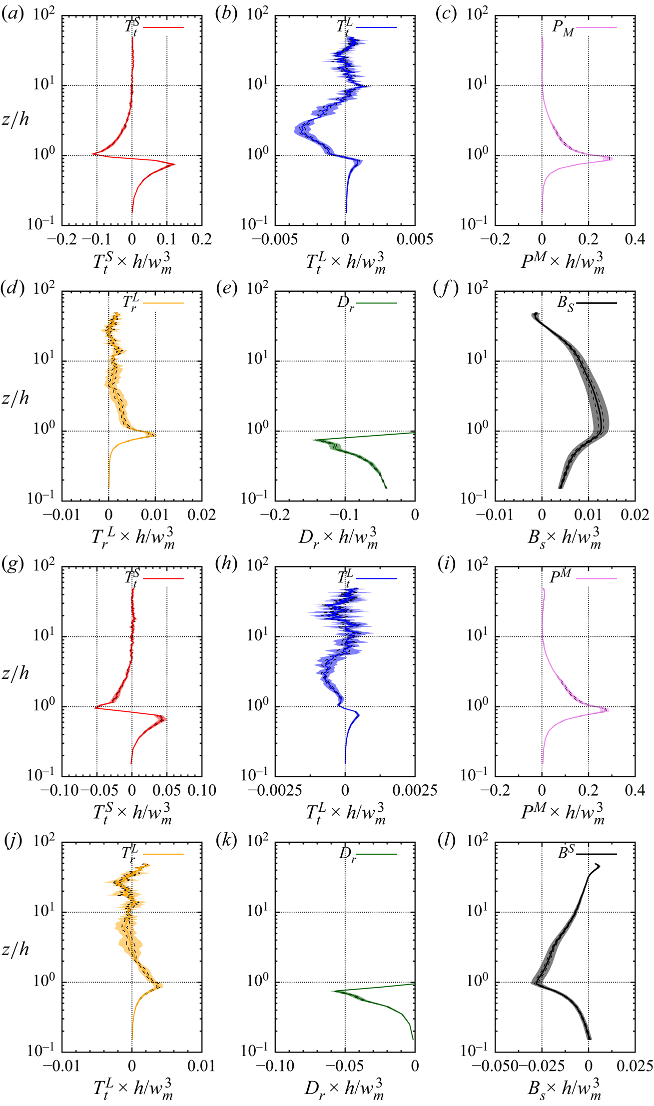
Figure 17. Confidence interval of the mean interscale transfer terms  $T_t^S, T_t^L, P^M, T_r^L, D_r$ and
  $B_S$ of (
 $a$,
$a$, $b$,
$b$, $c$,
$c$, $d$,
$d$, $e$,
$e$, $f$) the small-scale TKE
  $(\xi ^S)^2$ and (
 $g$,
$g$, $h$,
$h$, $i$,
$i$, $j$,
$j$, $k$,
$k$, $l$) the small-scale RSS
  $-u^S w^S$, for the WU case. The black dashed lines and the shaded areas show the 75 % and 95 % confidence bounds, respectively. The solid lines show the average values obtained from the
  $N_v=4$ LES volumes, as shown in figure 10(
 $a$,
$a$, $c$).
$c$).
Statistical error impacts mostly the terms of smallest amplitude, namely  $T_t^L$ and
  $T_r^L$ (figures 17
 $c$,
$c$, $d$ and 17
 $g$,
$g$, $f$, respectively). Nevertheless, the wall-normal evolution of these terms, particularly their change of sign, as discussed in § 3, remain valid and significant. The same applies for the other atmospheric stability configurations (not shown here).