


1. Introduction
Crustal stress within volcano-tectonic settings is the result of a combination of regional tectonic stresses, the geometry of local pressurized magma bodies (Pollard & Muller, Reference Pollard and Muller1976; Gudmundsson, Reference Gudmundsson2020) and the mechanical properties of the host rock, in particular associated to layering (Bazargan & Gudmundsson, Reference Bazargan and Gudmundsson2019, Reference Bazargan and Gudmundsson2020). The nature of the competing interactions between tectonic and volcanic processes remains a challenge to understand due to the different space and time windows in which they occur. Progress in understanding the interplay between tectonic and volcanic processes has been made using modern techniques such as geodetic, photogrammetric and geological surveys (Knopf, Reference Knopf1936; Chadwick & Howard, Reference Chadwick and Howard1991), as well as investigations of crustal stress using theoretical models (Yamakawa, Reference Yamakawa1955; Mogi, Reference Mogi1959; Pollard, Reference Pollard, Halls and Fahrig1987; Okada, Reference Okada1992; Rubin, Reference Rubin1995; Pinel & Jaupart, Reference Pinel and Jaupart2004; Gudmundsson & Andrew, Reference Gudmundsson and Andrew2007).
A typical volcanic system consists of a volcanic edifice, perhaps associated with a collapse caldera, an active shallow magma chamber supplying the edifice with magma through dykes, and a deeper magma accumulation zone or magma reservoir (Fig. 1). When the pressure of the magma chamber exceeds the host rock strength, dykes will initiate and propagate toward the surface, either reaching it as eruptive fissures or being arrested or deflected into sills (Gudmundsson, Reference Gudmundsson2012). As they find their way to the surface, dykes will propagate orthogonal to the minimum local principal stress (Anderson, Reference Anderson1951). They are therefore markers of past or present-day spatially heterogeneous stress fields in volcanic regions (Nakamura et al. Reference Nakamura, Jacob and Davies1977; Chadwick & Howard, Reference Chadwick and Howard1991; Rubin, Reference Rubin1995). Consequently, dykes appear to be ideal candidates for recovering past or present-day stress fields that result from the interaction of tectonic stress and the driving pressure in magma chambers (Odé, Reference Odé1957; Muller & Pollard, Reference Muller and Pollard1977).
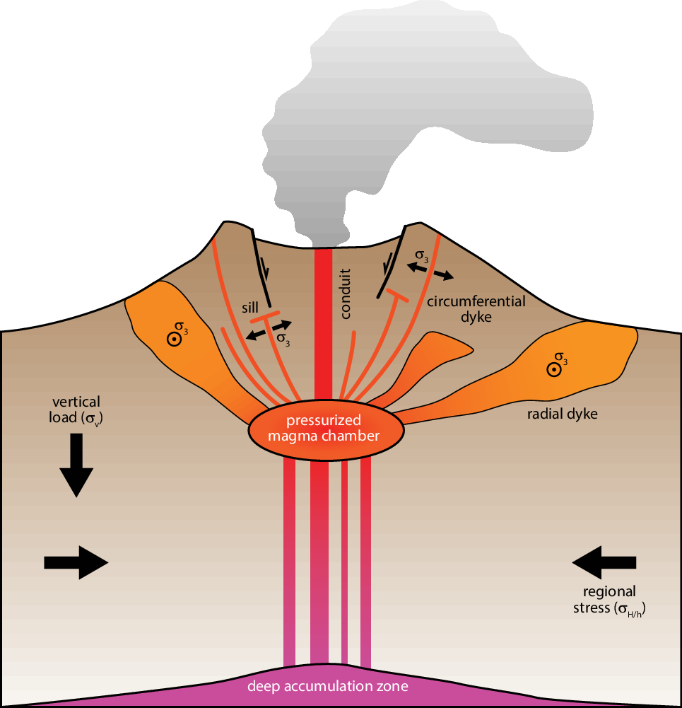
Fig. 1. Schematic illustration of a volcanic edifice and its associated caldera bounded by faults. The deeper accumulation zone feeds the shallower magma chamber through dykes. The magma chamber is the essential component to the volcanic system. Its driving pressure, once exceeding the rock strength, will lead to the initiation and propagation of dykes, not all of which will reach the surface.
Stress inversion methods have been widely used to study the crustal stress in volcano-tectonic settings (Bergerat, Reference Bergerat1987; Michael, Reference Michael1987; Angelier, Reference Angelier1994; Bauve et al. Reference Bauve, Plateaux, Rolland, Sanchez, Bethoux, Delouis and Darnault2014; Plateaux et al. Reference Plateaux, Béthoux, Bergerat and de Lépinay2014; Sigmundsson et al. Reference Sigmundsson, Hooper, Hreinsdóttir, Vogfjörd, Ófeigsson, Heimisson, Dumont, Parks, Spaans, Gudmundsson, Drouin, Árnadóttir, Jónsdóttir, Gudmundsson, Högnadóttir, Fridriksdóttir, Hensch, Einarsson, Magnússon and Eibl2014) and can be used to recover the past or present-day regional stresses from observed fault and dyke patterns. However, these classic formulations of stress inversion, based on observed fault characteristics, assume that a change of the volumetric stress tensor (i.e. isotropic or hydrostatic stress) has no effect on the fault slip direction and magnitude (et al.Angelier, Reference Angelier1979, Reference Angelier1994. Reference Angelier2002; Etchecopar et al. Reference Etchecopar, Vasseur and Daignieres1981; Michael, Reference Michael1984, Reference Michael1987). Indeed, such formulations implicitly assume that discontinuities (i.e. faults, magma chambers, salt diapirs, etc.) cannot open or close. In the case of pressurized cavities, however, the effect of the volumetric part of the stress tensor cannot be neglected as it may affect the resulting displacement (Maerten et al. Reference Maerten, Maerten and Lejri2018). Muller (Reference Muller1986) and Baer and Reches (Reference Baer and Reches1991) have developed interesting inversion methods that take into account volumetric change to recover both the regional stress and magma pressure. They used two-dimensional elastic analytic solutions of a pressurized circular hole subjected to a far field stress as proxy for the magmatic intrusion. Sets of stress trajectories are computed and compared to observed dyke trajectories over a wide range of parameters such as the far field stress magnitude and orientation, the radius of the magma intrusion and its location. While the technique has proven to be efficient, it is nonetheless limited to 2D simulations of circular intrusions.
In this contribution, we combine the efficiency of a linear elastic boundary element method (BEM) with an extended stress inversion formulation (F Maerten et al. Reference Maerten, Madden, Pollard and Maerten2016; L Maerten et al. Reference Maerten, Madden, Pollard and Maerten2016) based on the superposition principle to provide a multiparametric inversion scheme. This inversion takes into account the volumetric change associated with pressurized magma chambers of any 3D shapes and observational data such as observed dyke or eruptive fissure orientations. No attempt is made here to invert for the shape and position of the magma chambers. Instead, we assume geometric 3D shapes and locations based on previous studies.
First, we test the BEM against known analytical solutions and validate that it can be efficiently used to model pressurized cavities. Then we give a detailed description of the inversion methodology. Finally, two well-known study cases located in volcano-tectonic systems are used to test the multiparametric inversion method, namely the Spanish Peaks and the Galapagos Islands. In both examples, dyke trajectories are the main input to constrain the inversion to yield information on the direction and magnitude of the tectonic stress and internal pressure of magma chambers.
2. Method
The previous conceptual methodology used to recover far field tectonic stresses as well as the magma chamber pressure is to run thousands of simulations covering the range of all possible far field stress configurations and magma pressures. Then, for each simulation, one compares attributes of the modelled stresses with the dyke geometry (i.e. strike and dip) where they are observed. Finally, the simulations that give the best fit between modelled stresses and observed dykes are selected as the optimum models.
This method is based on the following assumptions:
-
1. Dyke trajectories used to constrain the inversion must have followed the past ambient stresses that are a combination of local stresses near pressurized magma chamber and far field tectonic stresses (Odé, Reference Odé1957; Muller & Pollard, Reference Muller and Pollard1977; Muller, Reference Muller1986; Baer & Reches, Reference Baer and Reches1991).
-
2. No other important mechanisms must have constrained the observed dyke propagation paths: for instance, pre-existing fractures or anisotropic materials (e.g. layering) that could deviate dyke paths from the ambient stresses (Jolly & Sanderson, Reference Jolly and Sanderson1995; Gudmundsson, Reference Gudmundsson2011).
2.a. Superposition principle, linear elasticity and BEM
The key idea to efficiently invert for both the tectonic stresses and the pressure in magma chambers while reducing the computation time associated with thousands of simulations is to apply the superposition principle (Brillouin, Reference Brillouin1946). This principle states that for any linear system, two or more solutions can be added together so that their weighted sum is also a solution. The use of this principle allows recovery of the displacement, strain and stress anywhere in a model using pre-computed specific values from linearly independent simulations.
In this study we use linear elastic models in our geomechanical simulations to be capable of applying the superposition principle. The use of linear elasticity for modelling deformation and fractures is supported by numerous research studies over the past half-century. These studies have used linear elasticity to effectively explain observed geological structures such as fractures (Kattenhorn et al. Reference Kattenhorn, Aydin and Pollard2000; Bourne & Willemse, Reference Bourne and Willemse2001), veins (Soliva et al. Reference Soliva, Maerten, Petit and Auzias2010), dykes (Odé, Reference Odé1957; Muller & Pollard, Reference Muller and Pollard1977; Baer & Reches, Reference Baer and Reches1991), fault slip (Maerten, Reference Maerten2000), fault-related deformation (Maerten et al. Reference Maerten, Pollard and Karpuz2000) and even salt-related deformation (Luo et al. Reference Luo, Nikolinakou, Flemings and Hudec2012). We therefore believe that such mechanical elastic behaviour is appropriate as a first approximation for modelling dyke propagation from magma chambers or stocks.
Several 3D numerical methods can be used with this methodology, such as the finite element method (FEM), the finite difference method (FDM) or the boundary element method (BEM). We decided to adopt the BEM because it has already proven to be useful for far field stress inversion (Kaven et al. Reference Kaven, Maerten and Pollard2011; F Maerten et al. Reference Maerten, Madden, Pollard and Maerten2016). In addition, it has a feature that is better suited for the proposed multiparametric inversion method: only the 3D surfaces representing displacement discontinuities such as fractures, cavities, intrusions and bedding interfaces have to be defined as triangulated surfaces while the volume of the model does not have to be built and meshed explicitly.
We have therefore developed and used a BEM called ARCH, which has the same foundations as Poly3D (Thomas, Reference Thomas1993; Maerten et al. Reference Maerten, Resor, Pollard and Maerten2005) and iBem3D (Maerten et al. Reference Maerten, Maerten and Pollard2014), except that it has been optimized and it incorporates the singularity corrections identified by Nikkhoo and Walter (Reference Nikkhoo and Walter2015). In the proposed method we assume that a magma chamber or a stock can be compared to a pressurized cavity with prescribed traction boundary conditions. Therefore, to validate that the BEM numerical technique can model pressurized cavities, we benchmarked this method against the closed form solution of a pressurized cylindrical body subjected to a 3D far field stress (Fjaer et al. Reference Fjaer, Holt, Horsrud and Raaen2008). This solution allows computing the stress at a given point around a pressurized cylindrical cavity (see Supplementary Material 1, available online at https://doi.org/10.1017/S001675682200067X). The BEM approach validates against the known analytical 3D solution of a pressurized cylinder subjected to a 3D far field stress, showing a perfect agreement between the two solutions.
2.b. Definition of the parameter space
The three main unknowns for geomechanically studying volcanoes and their associated deformation are (1) the magma chamber geometry, (2) the far field tectonic stresses and (3) the magma density and excess pressure. In this contribution, we did not invert for the shape and position of the magma chambers, but instead used simple assumptions based on previous work. In the following section, we therefore exclusively concentrate on unknowns (2) and (3) and define all the associated parameters that we called the parameter space.
2.b.1. Far field stress and local boundary conditions
In most previous stress inversion techniques (et al.Kaven et al. Reference Kaven, Maerten and Pollard2011; Célérier et al. Reference Célérier, Etchecopar, Bergerat, Vergely, Arthaud and Laurent2012; F Maerten et al. Reference Maerten, Madden, Pollard and Maerten2016), the stress ratio (Angelier, Reference Angelier1979) is solely used to describe the change in shape of the stress ellipsoid. These inversion techniques are implicitly based on the hypothesis that fault walls are constrained to slip without the possibility to overlap or open. This is schematically illustrated in 2D in Figure 2a, b, where a faulted block will slide in response to either (i) a vertical compression (Fig. 2a) or (ii) a horizontal tension (Fig. 2b). If we assume that the fault walls cannot open or overlap, (i) and (ii) are equivalent and the notion of stress ratio can be introduced within the far field stress tensor as a unique parameter.

Fig. 2. A 2D faulted block with normal slip which can be the result of (a) a vertical compressive stress or (b) a horizontal tensile stress. In both cases, one must assume that the fault walls cannot overlap or open. When overlapping or opening is allowed, the result of a vertical compression (c) or a horizontal tension (d) is fundamentally different from (a) and (b).
In three dimensions, the regional stress is written as follow:
 \begin{align}{\sigma _R} &= \boldsymbol{Q}\left[ {\matrix{
{{\sigma _1} - {p_p}} & {} & {} \cr
{} & {{\sigma _2} - {p_p}} & {} \cr
{} & {} & {{\sigma _3} - {p_p}} \cr
} } \right]{\kern 1pt} \,\boldsymbol{Q}^{T} = ({\sigma _1} - {\sigma _3})\,\boldsymbol{Q}\left[ {\matrix{
1 & {} & {} \cr
{} & R & {} \cr
{} & {} & 0 \cr
} } \right]\boldsymbol{Q}^{T}\\
&\quad - ({p_p} - {\sigma _3}){I_3} \equiv \boldsymbol{Q}\left[ {\matrix{
1 & {} & {} \cr
{} & R & {} \cr
{} & {} & 0 \cr
} } \right]\boldsymbol{Q}^{T}\end{align}
\begin{align}{\sigma _R} &= \boldsymbol{Q}\left[ {\matrix{
{{\sigma _1} - {p_p}} & {} & {} \cr
{} & {{\sigma _2} - {p_p}} & {} \cr
{} & {} & {{\sigma _3} - {p_p}} \cr
} } \right]{\kern 1pt} \,\boldsymbol{Q}^{T} = ({\sigma _1} - {\sigma _3})\,\boldsymbol{Q}\left[ {\matrix{
1 & {} & {} \cr
{} & R & {} \cr
{} & {} & 0 \cr
} } \right]\boldsymbol{Q}^{T}\\
&\quad - ({p_p} - {\sigma _3}){I_3} \equiv \boldsymbol{Q}\left[ {\matrix{
1 & {} & {} \cr
{} & R & {} \cr
{} & {} & 0 \cr
} } \right]\boldsymbol{Q}^{T}\end{align}
where
 $R = \left( {{\sigma _2} - {\sigma _3}} \right)/\left( {{\sigma _1} - {\sigma _3}} \right)$
is the stress ratio,
$R = \left( {{\sigma _2} - {\sigma _3}} \right)/\left( {{\sigma _1} - {\sigma _3}} \right)$
is the stress ratio,
 $Q$
is the 3D rotation matrix containing the three Euler angles
$Q$
is the 3D rotation matrix containing the three Euler angles
 $\left( {\varphi ,\theta ,\psi } \right)$
, and
$\left( {\varphi ,\theta ,\psi } \right)$
, and
 ${p_p}$
the pore pressure. As previously mentioned, the first simplification in Equation 1 comes from the fact that the isotropic part of the stress tensor,
${p_p}$
the pore pressure. As previously mentioned, the first simplification in Equation 1 comes from the fact that the isotropic part of the stress tensor,
 $\left( {{p_p} - {\sigma _3}} \right){I _3}$
, will not influence the fault slip direction and magnitude. Therefore, only the deviatoric part contributes to the shear stress since the isotropic pressure part results in a force normal to any plane. Similarly, the scaling coefficient given by the maximum differential stress,
$\left( {{p_p} - {\sigma _3}} \right){I _3}$
, will not influence the fault slip direction and magnitude. Therefore, only the deviatoric part contributes to the shear stress since the isotropic pressure part results in a force normal to any plane. Similarly, the scaling coefficient given by the maximum differential stress,
 $\left( {{\sigma _1} - {\sigma _3}} \right),$
only affects the fault slip magnitudes, not the directions. Therefore, it is discarded as a second simplification.
$\left( {{\sigma _1} - {\sigma _3}} \right),$
only affects the fault slip magnitudes, not the directions. Therefore, it is discarded as a second simplification.
However, if we allow either opening or overlapping of the discontinuity walls with a displacement perpendicular to the walls (e.g. a change in volume), the resulting displacements and stress fields are substantially different. The most common opening-mode discontinuities in nature are the joints, veins (tension gashes) and dykes but they also include inflating magma chambers, salt bodies or cavities caused by increased pressure. The most typical natural overlapping mode discontinuities are compaction bands and dissolution seams (stylolites) but they also include deflating magma chambers, salt bodies or cavities caused by a decreased internal pressure.
To better illustrate this effect, we performed a 3D numerical model of the cases presented in Fig. 2, representing an inclined fault subjected to a uniaxial tension or compression in the x–y plane. In Figure 3a, b, the fault is subjected to a traction boundary condition in the fault plane such that it is free to slip, and has imposed zero displacement in the normal direction to the fault plane to prevent any opening or overlapping of the fault walls. In such a configuration, applying a compression along the y-axis (Fig. 3a) or a tension along the x-axis (Fig. 3b) gives similar contours of the displacement norm around the fault. In contrast, in Figure 3c, d the fault is subjected to traction boundary conditions in all three local directions (both perpendicular and parallel to the fault plane). Consequently, the fault walls are still free to shear, but also free to overlap or open. Applying a compression (Fig. 3c) or a tension (Fig. 3d) now gives different results in terms of normalized displacement fields compared to Figure 3a, b.

Fig. 3. Effect of fault slip on the predicted displacement field norm using uniaxial remote loadings. The predicted results give similar iso-contours when shearing is only permitted with uniaxial compression (a) or tension (b). In contrast, the predicted results give different iso-contours when opening or overlapping of the fault walls is permitted with uniaxial compression (c) or tension (d).
In Maerten et al. (Reference Maerten, Maerten and Lejri2018), a similar conclusion was presented using modelled
 ${\sigma _1}$
trajectories, and that was compared with experiments done in PMMA (polymethyl methacrylate) containing open defects subjected to compression (de Joussineau et al. Reference De Joussineau, Petit and Gauthier2003). By allowing overlapping or opening of fault walls, a vertical compression or a horizontal tension leads to different results (Figs 2c, 3c and 2d, 3d, respectively). This is also demonstrated in Jaeger et al. (Reference Jaeger, Cook and Zimmerman2009: 249–50) where the stress distribution along the edge of a penny-shaped crack subjected to shear and/or opening is analytically formulated (i.e. equations 8.313–8.323). These equations demonstrate that adding opening or interpenetration during shearing gives different results than when modelling shearing only.
${\sigma _1}$
trajectories, and that was compared with experiments done in PMMA (polymethyl methacrylate) containing open defects subjected to compression (de Joussineau et al. Reference De Joussineau, Petit and Gauthier2003). By allowing overlapping or opening of fault walls, a vertical compression or a horizontal tension leads to different results (Figs 2c, 3c and 2d, 3d, respectively). This is also demonstrated in Jaeger et al. (Reference Jaeger, Cook and Zimmerman2009: 249–50) where the stress distribution along the edge of a penny-shaped crack subjected to shear and/or opening is analytically formulated (i.e. equations 8.313–8.323). These equations demonstrate that adding opening or interpenetration during shearing gives different results than when modelling shearing only.
Consequently, the reduced stress tensor cannot be used solely for modelling pressurized discontinuities as we must impose traction boundary conditions in the normal direction of discontinuities, which in turn implies a potential change in volume. Equation 1 is rewritten accordingly
 $${\sigma _R} = \left( {{\sigma _1} - {\sigma _3}} \right)\left( {{\rm{Q}}\left[ {\matrix{
1 & {} & {} \cr
{} & {Rs} & {} \cr
{} & {} & 0 \cr
} } \right]{Q^T} - {R_v}{I_3}} \right)$$
$${\sigma _R} = \left( {{\sigma _1} - {\sigma _3}} \right)\left( {{\rm{Q}}\left[ {\matrix{
1 & {} & {} \cr
{} & {Rs} & {} \cr
{} & {} & 0 \cr
} } \right]{Q^T} - {R_v}{I_3}} \right)$$
in which
 $$\left\{ {\matrix{ {{R_s} = \left( {{\sigma _2} - {\sigma _3}} \right)/\left( {{\sigma _1} - {\sigma _3}} \right)} \hfill \cr {{R_v} = \left( {{p_p} - {\sigma _3}} \right)/\left( {{\sigma _1} - {\sigma _3}} \right)} \hfill \cr } } \right.$$
In addition to
 $R \in \left[ {0,1} \right]$
, which we rename
$R \in \left[ {0,1} \right]$
, which we rename
 ${R_s}$
with the subscript ‘s’for shear, we define the stress ratio
${R_s}$
with the subscript ‘s’for shear, we define the stress ratio
 ${R_v} \in \mathbb{R}$
for which the subscript ‘v’ stands for volumetric. The parameter space extends from
${R_v} \in \mathbb{R}$
for which the subscript ‘v’ stands for volumetric. The parameter space extends from
 ${\sigma _R}\left( {\varphi ,\theta ,\psi ,{R_s}} \right)$
to
${\sigma _R}\left( {\varphi ,\theta ,\psi ,{R_s}} \right)$
to
 ${\sigma _R}\left( {\varphi ,\theta ,\psi ,{R_s},{R_v}} \right)$
, with
${\sigma _R}\left( {\varphi ,\theta ,\psi ,{R_s},{R_v}} \right)$
, with
 $\varphi ,\theta ,\psi $
the three Euler angles.
$\varphi ,\theta ,\psi $
the three Euler angles.
2.b.2. Magma pressure
We now further define the total pressure (
 ${p_m}$
) inside a magma chamber as
${p_m}$
) inside a magma chamber as
 $${p_m}\left( z \right) = {p_e} + {\rho _m}g\left| z \right| = {p_e} + p\left( z \right)$$
where
 ${p_e}$
represents the excess pressure, i.e. the pressure of the chamber at depth
${p_e}$
represents the excess pressure, i.e. the pressure of the chamber at depth
 $z = 0$
, and
$z = 0$
, and
 $p\left( z \right)$
the isotropic magma pressure with
$p\left( z \right)$
the isotropic magma pressure with
 ${\rho _m}$
being the density of the magma in the chamber. We assume that the pressure can take any positive value (i.e. excess pressure) or negative value (i.e. deficient pressure). The total magma pressure,
${\rho _m}$
being the density of the magma in the chamber. We assume that the pressure can take any positive value (i.e. excess pressure) or negative value (i.e. deficient pressure). The total magma pressure,
 ${p_m}$
, is consequently the general formulation incorporating the excess pressure (Yun et al. Reference Yun, Segall and Zebker2006; Gudmundsson, Reference Gudmundsson2012), the isotropic magma pressure and the effect of the density contrast inside a magma chamber.
${p_m}$
, is consequently the general formulation incorporating the excess pressure (Yun et al. Reference Yun, Segall and Zebker2006; Gudmundsson, Reference Gudmundsson2012), the isotropic magma pressure and the effect of the density contrast inside a magma chamber.
2.c. Applying the superposition principle
Our goal is then to estimate, through the multiparametric inversion, the parameters
 ${p_e}$
and
${p_e}$
and
 ${\rho _m}$
(if not imposed), in addition to the far field stress parameters,
${\rho _m}$
(if not imposed), in addition to the far field stress parameters,
 ${\sigma _R}\left( {\varphi ,\theta ,\psi ,{R_s},{R_v}} \right)$
.
${\sigma _R}\left( {\varphi ,\theta ,\psi ,{R_s},{R_v}} \right)$
.
As stated above, using the principle of superposition, it is possible, given a number of linearly independent solutions of a model, to compute the solution for a change in pressure in a magma chamber, a change in magma or rock density, a change of the Young’s modulus or a change in the far field stress. To this end, the input parameters
 $\left( {\varphi ,\theta ,\psi ,{R_s},{R_v},{\rho _m},\;{p_e}} \right)$
are transformed into linear parameters (F Maerten et al. Reference Maerten, Madden, Pollard and Maerten2016)
$\left( {\varphi ,\theta ,\psi ,{R_s},{R_v},{\rho _m},\;{p_e}} \right)$
are transformed into linear parameters (F Maerten et al. Reference Maerten, Madden, Pollard and Maerten2016)
 $$ S = {\left\{ {{\sigma _R},{\rho _m},{p_e}} \right\}^T} = {\left\{ {{\sigma _{xx}},{\sigma _{xy}},{\sigma _{xz}},{\sigma _{yy}},{\sigma _{yz}},{\sigma _{zz}},{\rho _m},{p_e}} \right\}^T}$$
These constitute the eight independent simulations that must be performed for the inversion of the regional stresses and the excess pressure of one magma chamber. In Equation 5,
 ${\sigma _R}$
represents the components of the far field stress in the global coordinate system. Given eight initial linearly independent simulations, any far field stress, excess pressure and magma density can be written as a linear combination of these eight initial simulations:
${\sigma _R}$
represents the components of the far field stress in the global coordinate system. Given eight initial linearly independent simulations, any far field stress, excess pressure and magma density can be written as a linear combination of these eight initial simulations:
 $${\left\{ {{\sigma _R},{\rho _m},{p_e}} \right\}^T} = S = \left[ {{{ S_1} \ldots { S}_8}} \right]\left\{ {\matrix{ {{\alpha _1}} \cr \vdots \cr {{\alpha _8}} \cr } } \right\}= A\alpha$$
where each
 ${S_i}$
represents a column of a matrix
${S_i}$
represents a column of a matrix
 $A$
, i.e. different linearly independent boundary conditions and model parameters applied to the model (far field stress, excess pressure and magma density) for the initial simulations. By linearly independent simulations, we mean that a simulation cannot be written as a linear combination of other simulations. In other words, the equation
$A$
, i.e. different linearly independent boundary conditions and model parameters applied to the model (far field stress, excess pressure and magma density) for the initial simulations. By linearly independent simulations, we mean that a simulation cannot be written as a linear combination of other simulations. In other words, the equation
 $\mathop \sum \nolimits_{i = 1}^8 {\alpha _i}{S_i} = 0$
can only be satisfied when
$\mathop \sum \nolimits_{i = 1}^8 {\alpha _i}{S_i} = 0$
can only be satisfied when
 ${\alpha _i} = 0$
for
${\alpha _i} = 0$
for
 $i \in \left[ {1,\;8} \right]$
. As described in F Maerten et al. (Reference Maerten, Madden, Pollard and Maerten2016), the simplest and most stable way (in term of matrix condition) to choose the linearly independent remote stresses, magma density and excess pressure is such that
$i \in \left[ {1,\;8} \right]$
. As described in F Maerten et al. (Reference Maerten, Madden, Pollard and Maerten2016), the simplest and most stable way (in term of matrix condition) to choose the linearly independent remote stresses, magma density and excess pressure is such that
 $A$
is the identity matrix, constituting the natural basis vectors of dimension eight. In that case, Equation 6 simplifies to
$A$
is the identity matrix, constituting the natural basis vectors of dimension eight. In that case, Equation 6 simplifies to
 $S = \alpha $
, and parameter
$S = \alpha $
, and parameter
 $\alpha $
represents both the linear coefficients for the superposition and the physical parameters
$\alpha $
represents both the linear coefficients for the superposition and the physical parameters
 $${\alpha} = \left\{ {{\sigma _{xx}},{\sigma _{xy}},{\sigma _{xz}},{\sigma _{yy}},{\sigma _{yz}},{\sigma _{zz}},{\rho _m},{p_e}} \right\}$$
If at a given observation point,
 $P$
, in the three-dimensional space, we store the total stress (i.e. the perturbed stress caused by pressurized magma chambers and any sliding faults, plus the far field stress) for the eight simulations,
$P$
, in the three-dimensional space, we store the total stress (i.e. the perturbed stress caused by pressurized magma chambers and any sliding faults, plus the far field stress) for the eight simulations,
 $\sigma _P^i$
, then the total stress at
$\sigma _P^i$
, then the total stress at
 $P$
for a given
$P$
for a given
 $\alpha $
is simply
$\alpha $
is simply
 ${\sigma _P} = \mathop \sum \nolimits_i {\alpha _i}\sigma _P^i$
. When a gradient is used for the far field stress and pressures, then all the initial simulations must be performed using the gradient as well.
${\sigma _P} = \mathop \sum \nolimits_i {\alpha _i}\sigma _P^i$
. When a gradient is used for the far field stress and pressures, then all the initial simulations must be performed using the gradient as well.
The superposition algorithm is summarized in Supplementary Material 2 and the case of multiple pressure inversion is described in Supplementary Material 3 (both available online at https://doi.org/10.1017/S001675682200067X).
In the following case studies, we have reduced the parameter space as follows. We assume that the magma density is known (
 ${\rho _m}$
= 2600 kg m−3). Therefore,
${\rho _m}$
= 2600 kg m−3). Therefore,
 ${\rho _m}$
is fixed in the parameter space. Then we assume that one of the principal stress directions is vertical (Anderson, Reference Anderson1905; Lisle et al. Reference Lisle, Orife, Arlegui, Liesa and Srivastava2006). Therefore, depending on which of the principal stresses is vertical, we can cover the normal, strike-slip and reverse fault stress regimes with
${\rho _m}$
is fixed in the parameter space. Then we assume that one of the principal stress directions is vertical (Anderson, Reference Anderson1905; Lisle et al. Reference Lisle, Orife, Arlegui, Liesa and Srivastava2006). Therefore, depending on which of the principal stresses is vertical, we can cover the normal, strike-slip and reverse fault stress regimes with
 ${\sigma _v} = {\sigma _1}$
,
${\sigma _v} = {\sigma _1}$
,
 ${\sigma _v} = {\sigma _2}$
and
${\sigma _v} = {\sigma _2}$
and
 ${\sigma _v} = {\sigma _3}$
respectively. This assumption implies that
${\sigma _v} = {\sigma _3}$
respectively. This assumption implies that
 ${\sigma _{xz}} = {\sigma _{yz}} = 0$
from the parameter space.
${\sigma _{xz}} = {\sigma _{yz}} = 0$
from the parameter space.
2.d. Inversion strategy and objective functions
As in F Maerten et al. (Reference Maerten, Madden, Pollard and Maerten2016) and L Maerten et al. (Reference Maerten, Madden, Pollard and Maerten2016), multiple types of weighted data can be used and combined to constrain the multiparametric inversion, under the condition that an objective function can be defined for each data type. Examples of such data are focal mechanisms (F Maerten et al. Reference Maerten, Madden, Pollard and Maerten2016), fractures (L Maerten et al. Reference Maerten, Madden, Pollard and Maerten2016), dykes or eruptive fissure orientations, interferometric synthetic aperture radar (InSAR), GPS, tiltmeter or micro-seismicity measurements (Maerten, Reference Maerten2010 a).
Then any search algorithm can be used to determine the best parameters (i.e.
 $\alpha $
) that minimize the objective functions. For instance, in F Maerten et al. (Reference Maerten, Madden, Pollard and Maerten2016) and L Maerten (Reference Maerten, Maerten, Lejri and Gillespie2016), a Monte Carlo approach was used where the parameter space was sampled randomly and the solution, which minimized the objective functions, was retained. Other search algorithms can be used such as the Bee (Pham et al. Reference Pham, Ghanbarzadeh, Koc, Otri, Rahim and Zaidi2005) or the Ant (Dorigo, Reference Dorigo1992) algorithms. It is worth mentioning that if a parameter is known, then the corresponding
$\alpha $
) that minimize the objective functions. For instance, in F Maerten et al. (Reference Maerten, Madden, Pollard and Maerten2016) and L Maerten (Reference Maerten, Maerten, Lejri and Gillespie2016), a Monte Carlo approach was used where the parameter space was sampled randomly and the solution, which minimized the objective functions, was retained. Other search algorithms can be used such as the Bee (Pham et al. Reference Pham, Ghanbarzadeh, Koc, Otri, Rahim and Zaidi2005) or the Ant (Dorigo, Reference Dorigo1992) algorithms. It is worth mentioning that if a parameter is known, then the corresponding
 ${\alpha _i}$
is set accordingly and kept fixed while using a search algorithm. Similarly, unknown
${\alpha _i}$
is set accordingly and kept fixed while using a search algorithm. Similarly, unknown
 ${\alpha _i}$
can be bounded in the parameter space if necessary.
${\alpha _i}$
can be bounded in the parameter space if necessary.
In the following case studies, we define the objective function for a dyke located at
 ${P_i}$
such that the computed local minimum principal direction of the perturbed stress (geologist convention),
${P_i}$
such that the computed local minimum principal direction of the perturbed stress (geologist convention),
 ${\sigma _3}$
, is aligned with the normal
${\sigma _3}$
, is aligned with the normal
 $n$
direction, perpendicular to the observed dyke
$n$
direction, perpendicular to the observed dyke
 $${f_i} = {{2{w_i}} \over \pi }{\cos ^{ - 1}}\left| {{\sigma _3}. n} \right|\;$$
In Equation 8,
 w_i
represents the weight of the dyke and ‘.’ represents the dot product. The absolute value is taken since the normal can be defined on either side of the dyke. This objective function is zero when
w_i
represents the weight of the dyke and ‘.’ represents the dot product. The absolute value is taken since the normal can be defined on either side of the dyke. This objective function is zero when
 ${\sigma _3}$
is collinear with
${\sigma _3}$
is collinear with
 $n$
. When using dyke traces, the z component of both
$n$
. When using dyke traces, the z component of both
 ${\sigma _3}$
and
${\sigma _3}$
and
 $n$
is set to zero (i.e. projected onto a horizontal plane) and the two vectors are normalized before using Equation 8.
$n$
is set to zero (i.e. projected onto a horizontal plane) and the two vectors are normalized before using Equation 8.
3. Case studies
We have chosen two natural examples of magma intrusion at volcanoes that are known to display associated dykes for which the propagation path is believed to be affected by both local and regional stress fields. Our goal is to use these two examples as a proof of concept of the method described above. We do not discuss in any depth the geological evolution of these two case studies.
3.a. Spanish Peaks
The Spanish Peaks area is located in south-central Colorado, USA (Fig. 4), and is famous for its well-exposed radial dyke system. The two prominent topographic features composed of igneous, metamorphosed and deformed sedimentary rocks are the West and East Spanish Peaks. The peak intrusions, often referred as stocks (Johnson, Reference Johnson1961), were emplaced during late Oligocene to early Miocene time (Armstrong, Reference Armstrong1969; Stormer, Reference Stormer1972; Smith, Reference Smith1975, Reference Smith1978). Rocks of both peaks and the surrounding dykes produced the remarkable relief when exhumed due to regional uplift and erosion, being more resistant to weathering than the surrounding sedimentary rocks.

Fig. 4. Map of syenite and syenodiorite dykes (solid lines) in the Spanish Peaks region of south-central Colorado (USA) from Johnson (Reference Johnson1968) over topography (coloured by elevation). Closed dashed lines are the boundaries of igneous intrusive rock (the Spanish Peaks stock).
The numerous sub-vertical dykes that crop out around the peaks were first described by Hills (Reference Hills1901) and originally mapped out by Knopf (Reference Knopf1936). They vary from 1 to 30 m in thickness and are exposed for distances of up to 20 km. The dykes are divided into three distinct groups: independent, subparallel and radial dykes (Johnson, Reference Johnson1968). The radial dykes are syenite and syenodiorite and are focused approximately on West Spanish Peak (Fig. 4).
Since its first description, the radial dyke pattern at Spanish Peaks has been the subject of several hypotheses regarding its genesis and development. Hills (Reference Hills1901) supposed that dykes adjacent to the West Spanish Peak filled radial fractures formed during doming of the sedimentary rocks by the emplacement of the stocks. Knopf (Reference Knopf1936) thought that the possible ‘cause for this swinging around to an east–west direction is that the forces that, near the stocks, produced the radial fissuring, opened up, at a greater distance from the stocks, the latent tension fissures produced during the compression that had folded the sedimentary beds into a broad syncline before the stocks were injected, i.e. the dykes availed themselves of latent tension breaks across the axis of the fold’. Following Knopf’s idea, Johnson (Reference Johnson1961) argued that selective magma intrusion into pre-existing complex fracture sets could have accounted for the observed dyke patterns. These fracture sets could be the result of successive orogenic stresses of varying direction and magnitude during folding of the syncline before intrusion of the stocks. In Odé (Reference Odé1957), the similarity between the Spanish Peaks radial dyke pattern and the pattern of maximum principal stress trajectories for a particular elastic model was noted and an explanation that relates the dyke pattern to a model stress field was proposed. It is based on Anderson’s (Reference Anderson1951) postulate that dykes follow trajectories normal to the direction of the least principal stress. Odé's work suggests that the stress trajectories were mainly controlled by the stock, the Sangre de Cristo Range to the West, as well as the maximum principal regional stress orientation. Therefore, his model consisted of a pressurized circular hole – the West Spanish Peak stock – adjacent to a rigid, planar boundary – the Sangre de Cristo Range to the west – in a 2D elastic plate. On this stress system he superimposed a homogeneous far field stress having principal stresses parallel and perpendicular to the rigid boundary. The far field stresses simulated the regional stress state in the horizontal plane at the time of intrusion. Muller and Pollard (Reference Muller and Pollard1977) and Muller (Reference Muller1986) further explored Odé’s model by adding a far field oblique stress to the Sangre de Cristo Range rigid boundary, producing stress trajectories that mimic the dyke pattern remarkably well.
3.a.1. Spanish Peaks model configuration
Here, we adopt Odé’s stress hypothesis, and we apply the multiparametric inversion technique described above to the Spanish Peaks radial dyke pattern to find the optimum mechanical parameters when the magma intrusion and dykes were emplaced: (1) the magma pressure, (2) the orientation of the maximum horizontal far field stress and (3) the relative magnitude of the two far field horizontal stresses.
While our geomechanical simulations are in 3D, we nonetheless model the West Spanish Peak stock as a vertical cylindrical body (Fig. 5a) in a whole elastic space (Muller & Pollard, Reference Muller and Pollard1977) that is equivalent to a 2D model, where the vertical cylindrical body is long enough to reduce the upper and lower edge effects. The modelled stock radius is 1.4 km, instead of the 2.6 km used by Muller and Pollard (Reference Muller and Pollard1977), to prevent the observed dykes from being inside the modelled stock (Fig. 5b). No other geological information is available to constrain the idealized stock geometry.

Fig. 5. Spanish Peaks model configuration. (a) 3D view of the vertical cylinder with a radius of 1.4 km used to model the west Spanish Peaks stock. (b) Map view of observed dykes colour-coded with respect to the weight (w) used to constrain the multiparametric inversion.
We used a value of 0.25 for Poisson’s ratio (
 $\nu $
) and 30 GPa for Young’s Modulus (
$\nu $
) and 30 GPa for Young’s Modulus (
 $E$
), which are the mean values representative for sediments.
$E$
), which are the mean values representative for sediments.
In this pseudo-2D mechanical simulation the vertical far field stress has no effect on the results. The Andersonian 3D far field stress is defined by the two horizontal stresses that are normalized with respect to
 ${\sigma _v}$
such that
${\sigma _v}$
such that
 ${k_H} = {{{\sigma _H}} \over {{\sigma _v}}}$
and
${k_H} = {{{\sigma _H}} \over {{\sigma _v}}}$
and
 ${k_h} = {{{\sigma _h}} \over {{\sigma _v}}}$
. Therefore, the modelled far field stress consists of the relative magnitudes of the two horizontal stresses,
${k_h} = {{{\sigma _h}} \over {{\sigma _v}}}$
. Therefore, the modelled far field stress consists of the relative magnitudes of the two horizontal stresses,
 ${\sigma _H}$
and
${\sigma _H}$
and
 ${\sigma _h}$
, as well as the orientation (
${\sigma _h}$
, as well as the orientation (
 $\theta $
) of
$\theta $
) of
 ${\sigma _H}$
with respect to north. In our simulations, these far field stress parameters are unknowns of the multiparametric inversion process.
${\sigma _H}$
with respect to north. In our simulations, these far field stress parameters are unknowns of the multiparametric inversion process.
To simulate the magma pressure, a traction component normal to the cylinder surface (
 ${P_m}\left( z \right)$
) is initially set to allow inflation (i.e. positive traction) or deflation (i.e. negative traction) in response to both the imposed
${P_m}\left( z \right)$
) is initially set to allow inflation (i.e. positive traction) or deflation (i.e. negative traction) in response to both the imposed
 ${P_m}\left( z \right)$
and the far field stress. The two other initial traction components, parallel to the stock surface, are set to zero. In our simulations, we normalize the magma pressure with respect to
${P_m}\left( z \right)$
and the far field stress. The two other initial traction components, parallel to the stock surface, are set to zero. In our simulations, we normalize the magma pressure with respect to
 ${\sigma _v}$
such that
${\sigma _v}$
such that
 ${k_p} = {{{P_m}\left( z \right)} \over {{\sigma _v}}}$
. The ratio
${k_p} = {{{P_m}\left( z \right)} \over {{\sigma _v}}}$
. The ratio
 ${k_p}$
is therefore another unknown of the multiparametric inversion process.
${k_p}$
is therefore another unknown of the multiparametric inversion process.
In contrast to the models from Odé (Reference Odé1957) and Muller and Pollard (Reference Muller and Pollard1977), we did not attempt to model the effect of the Sangre de Cristo Range rigid boundary to the west.
The inversion process is constrained by the mapped sub-vertical dykes (Fig. 4) along with their known dip angle (∼90°) and azimuths. The dykes are placed at the mid-height of the vertical cylinder. The objective function used for the simulation is that described earlier for dykes.
Since this multiparametric inversion is solely constrained by the location, the dip and strike of the observed dykes, it is important to consider the fact that dykes are not necessarily evenly distributed or observed in the area (Fig. 4). This could have a significant effect on the far field stress inversion outcome as, for instance, a large concentration of radial dykes near the stock will downplay the effect of few curving dykes in the distance, which better indicate the regional stress orientation. We therefore decided not to give equal weight to each datum to account for the observed uneven dyke density. As illustrated in Fig.5b, the closely spaced western dykes in red observed between the cylinder and the Sangre de Cristo Range have a weight of 1/3, the southern dykes in green have a higher weight of 2/3 and the sparsely spaced northern dykes in blue have the highest weight of 1.
A horizontal observation grid, covering the entire study area, was placed at the mid-height of the vertical stock. A set of observation points, where we modelled potential dyke orientations derived from the computed perturbed stress field, are used to compare with the observed dyke patterns.
3.a.2. Spanish Peaks inversion results
To better visualize and analyse the results of the multiparametric inversion, we use a modified domain introduced by Muller (Reference Muller1986). This domain consists of a half-circular graph (Fig. 6e) for which the radius is the ratio defined as
 ${k_h}/{k_H}$
which goes from 1 to 0 and the angular coordinate defines the orientation (θ) of the maximum horizontal stress relative to north from 0° to 180°. Because the inversion was done for three parameters (
${k_h}/{k_H}$
which goes from 1 to 0 and the angular coordinate defines the orientation (θ) of the maximum horizontal stress relative to north from 0° to 180°. Because the inversion was done for three parameters (
 ${{{k_h}} \over {{k_H}}}$
,
${{{k_h}} \over {{k_H}}}$
,
 ${k_p}$
and
${k_p}$
and
 $\theta $
), we deliberately fixed
$\theta $
), we deliberately fixed
 ${k_p}$
to the optimum value found and only plot
${k_p}$
to the optimum value found and only plot
 ${k_h}/{k_H}$
versus
${k_h}/{k_H}$
versus
 $\theta $
. A point in the domain represents a single simulation; each simulation is coloured according to the mean misfit angle (
$\theta $
. A point in the domain represents a single simulation; each simulation is coloured according to the mean misfit angle (
 $\bar \delta $
) which is the arithmetic mean of all the misfit angles (
$\bar \delta $
) which is the arithmetic mean of all the misfit angles (
 $\delta $
) for all dykes.
$\delta $
) for all dykes.
 $\delta $
is the angle between the observed dyke strike direction,
$\delta $
is the angle between the observed dyke strike direction,
 ${d_o}$
, and the modelled dyke strike direction,
${d_o}$
, and the modelled dyke strike direction,
 ${d_m}$
, which varies from 0° to 90°, 0° being the best fit and 90° being the worst.
${d_m}$
, which varies from 0° to 90°, 0° being the best fit and 90° being the worst.

Fig. 6. Spanish Peaks model results. (a, b) Maps of observed dykes and modelled dyke trajectories for the optimum and example non-optimum model parameters respectively. Orange circles highlight the location of computed isotropic stresses where dyke trajectories cannot be defined. (c, d) Histograms of the misfit angles (δ) for the optimum and non-optimum model parameters, respectively. (e) Multiparametric inversion domain showing the location of the optimum (black circle) and non-optimum (white circle) models. The colour scale and contours show the mean misfit angle (
 $\bar \delta $
).
$\bar \delta $
).
It is defined as
 $$\delta = {{180} \over \pi }{\cos ^{ - 1}}\left| {d_0}.{d_m} \right|$$
The multiparametric inversion, which consists of six linearly independent forward simulations and 30 000 random geomechanical simulations, was run in less than 1 min (see Supplementary Material 4, available online at https://doi.org/10.1017/S001675682200067X). The optimum solution was found for a relative magma pressure
 ${k_p}$
=1.67, a far field maximum horizontal stress (
${k_p}$
=1.67, a far field maximum horizontal stress (
 ${\sigma _H}$
) oriented N81.2°E and a horizontal stress ratio
${\sigma _H}$
) oriented N81.2°E and a horizontal stress ratio
 ${{{k_h}} \over {{k_H}}}$
= 0.76, for a mean misfit angle
${{{k_h}} \over {{k_H}}}$
= 0.76, for a mean misfit angle
 $\bar \delta = 4.6^\circ $
. This result is highlighted in the multiparametric inversion domain with the green colours (black circle in Fig. 6e). Figure 6a shows a qualitative comparison between the observed dyke pattern and the modelled dyke trajectories derived from the stress field. Since dykes (i.e. opening-mode fractures) propagate in a plane normal to the local direction of the least compressive stress (i.e. σ3), the streamlines shown in Figure 6a represent the strike of the planes containing σ1 and σ2, which are mostly sub-vertical in this case. The modelled dyke trajectories show a good correspondence with the observed dyke pattern. Near the stock, the dyke trajectories converge to form a radial pattern but become more parallel to the far field stress,
$\bar \delta = 4.6^\circ $
. This result is highlighted in the multiparametric inversion domain with the green colours (black circle in Fig. 6e). Figure 6a shows a qualitative comparison between the observed dyke pattern and the modelled dyke trajectories derived from the stress field. Since dykes (i.e. opening-mode fractures) propagate in a plane normal to the local direction of the least compressive stress (i.e. σ3), the streamlines shown in Figure 6a represent the strike of the planes containing σ1 and σ2, which are mostly sub-vertical in this case. The modelled dyke trajectories show a good correspondence with the observed dyke pattern. Near the stock, the dyke trajectories converge to form a radial pattern but become more parallel to the far field stress,
 ${\sigma _H}$
= N81.2°E, at a greater distance (i.e. 20 km). The modelled dyke trajectories show one of the two unique points where their orientation is not defined (orange dot in Fig. 6a). These are referred to as isotropic stress points where
${\sigma _H}$
= N81.2°E, at a greater distance (i.e. 20 km). The modelled dyke trajectories show one of the two unique points where their orientation is not defined (orange dot in Fig. 6a). These are referred to as isotropic stress points where
 ${\sigma _h} = {\sigma _H}$
. This point, located to the north, does not fall at the Goemmer Butte (Fig. 4) as in the Muller and Pollard (Reference Muller and Pollard1977) model because the rigid boundary effect of the Sangre de Cristo Range has not been taken into account.
${\sigma _h} = {\sigma _H}$
. This point, located to the north, does not fall at the Goemmer Butte (Fig. 4) as in the Muller and Pollard (Reference Muller and Pollard1977) model because the rigid boundary effect of the Sangre de Cristo Range has not been taken into account.
3.a.3. Sensitivity to far field stress characteristics
We also evaluated the extent to which the modelled stress trajectories, hence the spatial distribution of the dykes around the West Spanish Peak stock, are sensitive to the far field stress characteristics. We arbitrarily chose a different but realistic far field state of stress (the ‘non-optimal’ results shown in Fig. 6b, d) for which
 ${\sigma _H}$
is oriented N30°E and the horizontal stress ratio
${\sigma _H}$
is oriented N30°E and the horizontal stress ratio
 ${{{k_h}} \over {{k_H}}} = 0.4$
. This is shown as a white circle in the multiparametric inversion domain of Figure 6e. The relative pressure
${{{k_h}} \over {{k_H}}} = 0.4$
. This is shown as a white circle in the multiparametric inversion domain of Figure 6e. The relative pressure
 ${k_p}$
inside the stock is the same as for the previous model.
${k_p}$
inside the stock is the same as for the previous model.
This model configuration gives a mean misfit angle
 $\bar \delta $
= 14.1°, which is almost three times higher than for the optimum model configuration. The histograms of the misfit angles, computed at each dyke segment for the two model configurations, are shown in Figure 6c, d. The general shape of the histograms is a good indicator of the goodness of fit: a flat histogram means that the fit is poor, whereas rapid decay with increasing misfit angle, as shown in the optimum model parameters of Figure 6c, means that the model fit is much better. Furthermore, the histogram of the optimum model parameters shows that 89.6 % of the observed dykes have a misfit angle less than 10°, whereas it is only 49.9 % for the non-optimum model.
$\bar \delta $
= 14.1°, which is almost three times higher than for the optimum model configuration. The histograms of the misfit angles, computed at each dyke segment for the two model configurations, are shown in Figure 6c, d. The general shape of the histograms is a good indicator of the goodness of fit: a flat histogram means that the fit is poor, whereas rapid decay with increasing misfit angle, as shown in the optimum model parameters of Figure 6c, means that the model fit is much better. Furthermore, the histogram of the optimum model parameters shows that 89.6 % of the observed dykes have a misfit angle less than 10°, whereas it is only 49.9 % for the non-optimum model.
Figure 6b illustrates a comparison between the non-optimum modelled dyke orientations and the observed dyke pattern. Again, the non-optimum modelled stress trajectories near the stock converge to radial, but at c. 10 km from the stock the modelled dyke trajectories become parallel to the far field stress (N30°E), and deviate from the observed dyke trajectories.
3.b. Galapagos Islands
The Galapagos archipelago is located at c. 1000 km west of Ecuador. It is a group of volcanic islands that are the product of a fixed oceanic hot spot under the Nazca plate. The formation of the Galapagos Islands is estimated at 3.9 Ma ago (Geist et al. Reference Geist, McBirney and Duncan1986). Due to the eastward motion of the Nazca plate, volcanoes are progressively younger and more active towards the west and the activity of the hot spot is now centred at Isabela and Fernandina islands (Fig. 7). In this case study, the seven active volcanoes of Isabela and Fernandina islands are considered for simulation, namely Fernandina, Ecuador, Wolf, Darwin, Alcedo, Sierra Negra and Cerro Azul volcanoes.

Fig. 7. Map of the eruptive fissures (solid lines) on Fernandina and Isabela islands of the Galapagos archipelago (Ecuador) over topography (colour scale). Modified from Chadwick and Howard (Reference Chadwick and Howard1991).
These basaltic shield volcanoes with large summit calderas are characterized by numerous linear eruptive fissures (Chadwick & Howard, Reference Chadwick and Howard1991), which are the result of dykes propagating from magma chambers beneath the calderas and intersecting the surface. These fissures (and their underlying dykes) display a very distinctive pattern that is circumferential around the calderas and radial on the flanks of the volcanoes (Fig. 7). This pattern of circumferential and radial dykes is intriguing because it is poorly documented on other basaltic shield volcanoes.
The longest eruptive fissure is c. 2.6 km, while the average is 0.6 km long. The radial eruptive fissures tend to concentrate between adjacent Galapagos volcanoes and diverge slightly to display a continuous pattern between volcanoes, suggesting coeval development (Fig. 7). This pattern is expected from the stress field interaction from two or more sources of pressurized magmatic chambers modified to some extent by regional stresses (Chadwick & Dieterich, Reference Chadwick and Dieterich1995). The radial eruptive fissure pattern observed in the Galapagos islands is somewhat similar to that in models used to explain dyke patterns at Spanish Peaks (Fig. 4).
The circumferential eruptive fissures in the Galapagos Islands are located within 1.5 km of caldera rims. They have often been interpreted as a direct consequence of the caldera faults channelling the magma to the surface (Nordlie, Reference Nordlie1973; Browning & Gudmundsson, Reference Browning and Gudmundsson2015) or as dyke propagation within a radially oriented stress field in the summit regions due to the steep topography of the caldera walls (Munro & Rowland, Reference Munro and Rowland1996). However, according to Chadwick and Howard (Reference Chadwick and Howard1991) ‘the circumferential fissures are not simply leaky faults, but their underlying dykes are emplaced as distinct and independent structures and require a specific stress field suitable for the observed fissure orientations’. Also, according to the same authors, the circumferential and radial eruptive fissures appear to have grown contemporaneously and are coexistent. Their interpretation is supported by the fact that (i) both circumferential and radial eruptions have occurred on individual Galapagos volcanoes in historical time, (ii) some individual eruptive fissures have a circumferential orientation near the caldera and gradually curve downslope to become radial and (iii) all fissures erupt the same tholeiite basalt (McBirney & Williams, Reference McBirney and Williams1969).
Other hypotheses have been developed to account for the contemporaneous development of both circumferential and radial eruptive fissures: (i) stress perturbations due to a pressurized magma chamber (Chadwick & Dieterich, Reference Chadwick and Dieterich1995; Bistacchi et al. Reference Bistacchi, Tibaldi, Pasquar and Rust2012; Chestler & Grosfils, Reference Chestler and Grosfils2013), (ii) stress perturbation caused by the gravitational unloading due to surface mass redistribution associated with the formation of a caldera (Corbi et al. Reference Corbi, Rivalta, Pinel, Maccaferri, Bagnardi and Acocella2015) and (iii) stress related to the loading of the volcanic edifice (Maccaferri et al. Reference Maccaferri, Bonafede and Rivalta2011; Rivalta et al. Reference Rivalta, Taisne, Bunger and Katz2015) by lava flow emplacement.
3.b.1 Galapagos model configuration
We are adopting the hypotheses that dykes will follow the ambient heterogeneous stress field produced by both the magma chamber pressurization and the regional stresses. As suggested by Pollard (Reference Pollard, Halls and Fahrig1987), it is not necessary that fractures occur before any dyking can take place, because dykes can create their own fractures which propagate immediately ahead of the advancing magma. We therefore apply the multiparametric inversion method described above to the Galapagos Islands dyke pattern to find the optimum mechanical parameters including: (1) the magma chamber pressure for each volcano, (2) the orientation of the maximum horizontal far field stress and (3) the magnitude of the two far field horizontal stresses and the stress regime.
The 3D model of the seven shallow magma chambers was built with oblate ellipsoids for which the horizontal dimensions (long and short axis) and their orientation are derived from the caldera shape of each volcano (Fig. 8). Their dimensions are reported in Table 1. The ratio of the longest axis over the vertical axis is the same for all magma chambers and set to 3.9. The depth of all magma chamber tops is fixed to 2000 m below sea level. These configurations, inspired by previous modelling work from several authors (Chadwick & Dieterich, Reference Chadwick and Dieterich1995; Yun et al. Reference Yun, Segall and Zebker2006; Chestler & Grosfils, Reference Chestler and Grosfils2013; Corbi et al. Reference Corbi, Rivalta, Pinel, Maccaferri, Bagnardi and Acocella2015), are probably not optimum shapes but they had to be defined for the inversion.

Fig. 8. Ellipsoid geometry of the modelled seven magma chambers. (a) Top view of the magma chambers and their respective locations with the observed eruptive fissures (black lines) used to constrain the multiparametric inversion. (b) Side view from the south of the Fernandina volcano and its modelled magma chamber. The 2D observation plane is placed at 600 m below sea level.
Table 1. Ellipsoid parameters of the seven magma chambers with a ratio of the longest axis over the vertical axis equal to 3.9 for all magma chambers

To simulate the magma pressure, a traction component normal to the magma chamber internal surface (
 ${P_m}\left( z \right)$
) is initially set. In contrast to the Spanish Peaks simulation, stress and pressure gradients are accounted for. The pressure applied on the chamber surfaces is the isotropic pressure of the magma (
${P_m}\left( z \right)$
) is initially set. In contrast to the Spanish Peaks simulation, stress and pressure gradients are accounted for. The pressure applied on the chamber surfaces is the isotropic pressure of the magma (
 ${\rho _m}g\left| z \right|$
) plus or minus a constant pressure (p
e
) depending on whether we model an inflating or a deflating chamber respectively and where
${\rho _m}g\left| z \right|$
) plus or minus a constant pressure (p
e
) depending on whether we model an inflating or a deflating chamber respectively and where
 ${\rho _m}$
is the magma density (
${\rho _m}$
is the magma density (
 ${\rho _m}$
= 2600 kg m−3),
${\rho _m}$
= 2600 kg m−3),
 $g$
is the gravitational constant and
$g$
is the gravitational constant and
 $z$
is the depth. The two other traction components, parallel to the chamber surfaces, are set to have initial tractions equal to 0. In our simulations,
$z$
is the depth. The two other traction components, parallel to the chamber surfaces, are set to have initial tractions equal to 0. In our simulations,
 ${p_e}$
is one of the unknowns of the multiparametric inversion process. However, since there are seven magma chambers, there is one
${p_e}$
is one of the unknowns of the multiparametric inversion process. However, since there are seven magma chambers, there is one
 ${p_e}$
per chamber, which makes seven unknowns instead of one in the Spanish Peaks model above.
${p_e}$
per chamber, which makes seven unknowns instead of one in the Spanish Peaks model above.
The Andersonian 3D far field stress is defined such that
 ${\sigma _v}$
is vertical compressive stress related to the overburden load such that
${\sigma _v}$
is vertical compressive stress related to the overburden load such that
 ${\sigma _v} = {\rho _{rock}}gz$
, where
${\sigma _v} = {\rho _{rock}}gz$
, where
 ${\rho _{rock}}$
is the mean rock density (
${\rho _{rock}}$
is the mean rock density (
 ${\rho _{rock}}$
= 2900 kg m−3) and
${\rho _{rock}}$
= 2900 kg m−3) and
 ${k_H}$
and
${k_H}$
and
 ${k_h}$
are defined as
${k_h}$
are defined as
 ${k_H} = {{{\sigma _H}} \over {{\sigma _v}}}$
and
${k_H} = {{{\sigma _H}} \over {{\sigma _v}}}$
and
 ${k_h} = {{{\sigma _h}} \over {{\sigma _v}}}$
, where
${k_h} = {{{\sigma _h}} \over {{\sigma _v}}}$
, where
 ${\sigma _H}$
and
${\sigma _H}$
and
 ${\sigma _h}$
are the maximum and minimum principal horizontal stresses respectively. Depending on the sign and relative magnitudes of
${\sigma _h}$
are the maximum and minimum principal horizontal stresses respectively. Depending on the sign and relative magnitudes of
 ${k_H}$
and
${k_H}$
and
 ${k_h}$
, a normal, strike-slip or reverse stress regime is modelled. Angle
${k_h}$
, a normal, strike-slip or reverse stress regime is modelled. Angle
 $\theta $
is defined as the orientation of
$\theta $
is defined as the orientation of
 ${\sigma _H}$
measured clockwise from north. In our simulations,
${\sigma _H}$
measured clockwise from north. In our simulations,
 ${k_H}$
,
${k_H}$
,
 ${k_h}$
and
${k_h}$
and
 $\theta $
are also unknowns of the multiparametric inversion process. In addition, an elastic half-space is used to take into account the traction-free effect of the Earth surface.
$\theta $
are also unknowns of the multiparametric inversion process. In addition, an elastic half-space is used to take into account the traction-free effect of the Earth surface.
The inversion process is constrained by the mapped eruptive fissures from Chadwick & Howard (Reference Chadwick and Howard1991) and updated by the authors with the interpretation of more recent satellite images available on Google Earth in the southern area of Isabella Island (see Fig. 7). As we assumed that the eruptive fissures represent the strikes of the underlying dykes and that no information is available regarding the dip of the dykes, only the strike of the fissures is used to constrain the inversion. Because the topography has not been included in our simulations, the eruptive fissures, measured on the volcano flanks, are projected onto a horizontal surface at −600 m elevation where a horizontal observation grid covering the two islands is placed.
The modelled dyke orientations on the observation grid are derived from the computed stress field, and are used to compare with the observed pattern of eruptive fissures. The objective function used for the simulation is that described earlier for opening-mode fractures.
In the following mechanical simulations, we use a homogeneous linear elastic and isotropic behaviour characterized by two constants, Poisson’s ratio and Young’s Modulus. We use a value of 0.25 for Poisson’s ratio (ν) and 30 GPa for Young’s Modulus (
 $E$
), which are the mean values representative for the surrounding rock.
$E$
), which are the mean values representative for the surrounding rock.
3.b.2. Galapagos inversion results
The multiparametric inversion, which consists of 12 pre-computed simulations and 30 000 random geomechanical simulations (see Supplementary Material 4, available online at https://doi.org/10.1017/S001675682200067X), gives the optimum solution with a mean misfit angle
 $\bar \delta = 13.6^\circ $
, between the orientation of the observed and the modelled dykes, which varies from 0° (best fit) to 90° (worst fit). The optimum solution also gives a far field maximum horizontal stress (
$\bar \delta = 13.6^\circ $
, between the orientation of the observed and the modelled dykes, which varies from 0° (best fit) to 90° (worst fit). The optimum solution also gives a far field maximum horizontal stress (
 ${\sigma _H}$
) oriented N89°E and a normal stress regime where
${\sigma _H}$
) oriented N89°E and a normal stress regime where
 ${k_H}$
= 0.381 and
${k_H}$
= 0.381 and
 ${k_h}$
= 0.378. This is very close to a uniaxial normal stress regime where
${k_h}$
= 0.378. This is very close to a uniaxial normal stress regime where
 ${\sigma _H} = {\sigma _h}$
. It is difficult to relate these inverted regional stress parameters to the actual stress field as very little is known about present-day stresses in the Galapagos.
${\sigma _H} = {\sigma _h}$
. It is difficult to relate these inverted regional stress parameters to the actual stress field as very little is known about present-day stresses in the Galapagos.
The inverted magma excess pressures (
 ${p_e}$
) for each volcano are shown in Table 2. The excess pressure at the time of dyke propagation is normally equal to the tensile strength of the host rock and is generally in the range of 0.5–6 MPa, up to about 9 MPa (Gudmundsson, Reference Gudmundsson2012). This pressure can be negative when there is a deflation of the magma chamber or collapse of the caldera. The inverted
${p_e}$
) for each volcano are shown in Table 2. The excess pressure at the time of dyke propagation is normally equal to the tensile strength of the host rock and is generally in the range of 0.5–6 MPa, up to about 9 MPa (Gudmundsson, Reference Gudmundsson2012). This pressure can be negative when there is a deflation of the magma chamber or collapse of the caldera. The inverted
 ${p_e}$
for all volcanoes are all positive (i.e. excess pressure) and fall within the range of tensile strength of the host rock with the smallest
${p_e}$
for all volcanoes are all positive (i.e. excess pressure) and fall within the range of tensile strength of the host rock with the smallest
 ${p_e}$
= 5.25 MPa for Alcedo volcano (one of the least active) and the highest
${p_e}$
= 5.25 MPa for Alcedo volcano (one of the least active) and the highest
 ${p_e}$
= 9.6 MPa for Fernandina volcano (one of the most active).
${p_e}$
= 9.6 MPa for Fernandina volcano (one of the most active).
Table 2. Inverted excess magma pressure
 ${p_e}$
on the seven Galapagos volcanoes
${p_e}$
on the seven Galapagos volcanoes

The optimum solution found from the multiparametric inversion is illustrated by the histogram of the misfit angles (
 $\delta $
), computed at each dyke segment (Fig. 9a). The histogram shows a rapid decay with increasing
$\delta $
), computed at each dyke segment (Fig. 9a). The histogram shows a rapid decay with increasing
 $\delta $
. Of the observed eruptive fissures, 69.4% have a
$\delta $
. Of the observed eruptive fissures, 69.4% have a
 $\delta $
that is less than 15° with the modelled dykes.
$\delta $
that is less than 15° with the modelled dykes.

Fig. 9. (a) Histograms of the misfit angles (δ) for the optimum model parameters. (b) Map of observed eruptive fissures (thick black lines) and modelled dyke trajectories (thin black lines) for the optimum Galapagos model parameters. Circles highlight the location of computed isotropic stresses where dyke trajectories cannot be defined.
Figure 9b shows a qualitative comparison between the observed pattern and the modelled dyke trajectories derived from the perturbed stress field. The modelled dyke trajectories show a good correspondence with the observed pattern of eruptive fissures. On the volcano flanks, the modelled and observed dyke trajectories converge toward the summit calderas, forming a well-defined radial pattern. On Fernandina Island the radial dykes tend to deviate from a purely radial trend at some distance from the caldera (i.e. 15 km). Their orientation may be affected by the regional stress field to the west and may be more affected by the nearby Darwin and Alcedo volcanoes to the east. The latter effect is even more pronounced between the Alcedo, Darwin, Wolf and Ecuador volcanoes where modelled and observed radial dykes show a continuous curving trend illustrating the clear mechanical interaction between contemporaneous volcanoes. The modelled dyke trajectories show several unique points where the orientation is not defined (orange dots in Fig. 9). These points, called isotropic stress points where local
 ${\sigma _h} = {\sigma _H}$
, are typical of perturbed stress field from several sources (i.e. magma chambers). Overall, there is not a very discernible effect of the regional stress on the modelled dyke trajectories as we are very close to a uniaxial normal stress regime where far field horizontal stress
${\sigma _h} = {\sigma _H}$
, are typical of perturbed stress field from several sources (i.e. magma chambers). Overall, there is not a very discernible effect of the regional stress on the modelled dyke trajectories as we are very close to a uniaxial normal stress regime where far field horizontal stress
 ${\sigma _h} \approx {\sigma _H}$
.
${\sigma _h} \approx {\sigma _H}$
.
The modelled dyke trajectories display a systematic circumferential dyke pattern above all the modelled magma chambers as observed in the field (Chadwick & Howard, Reference Chadwick and Howard1991). The presence of both radial and circumferential dykes in the geomechanical model illustrates that the development of both types of dykes can be contemporaneous as suggested by Chadwick and Howard (Reference Chadwick and Howard1991) and Chadwick and Dieterich (Reference Chadwick and Dieterich1995) from field observation and modelling respectively. Figure 10 illustrates the 3D nature of the modelled dyke trajectories over the Fernandina magma chamber. Since dykes (i.e. opening-mode fractures) propagate in a plane normal to the local direction of the least compressive stress (i.e.
 ${\sigma _3}$
), we represent the modelled dyke orientation as yellow discs (Fig. 10) whose normal is aligned with the local least compressive stress direction. The radial dykes are mostly but not exclusively sub-vertical in this case. However, the modelled circumferential dykes just above the magma chamber are dipping inward toward the caldera as observed in the field (Chadwick & Howard, Reference Chadwick and Howard1991).
${\sigma _3}$
), we represent the modelled dyke orientation as yellow discs (Fig. 10) whose normal is aligned with the local least compressive stress direction. The radial dykes are mostly but not exclusively sub-vertical in this case. However, the modelled circumferential dykes just above the magma chamber are dipping inward toward the caldera as observed in the field (Chadwick & Howard, Reference Chadwick and Howard1991).

Fig. 10. 3D perspective view of observed eruptive fissures at the surface (thick black lines), used to constrain the inversion, and modelled dyke orientations (yellow discs) above the Fernandina magma chamber (red ellipsoid). The modelled radial dykes are sub-vertical while the modelled circumferential dykes dip toward the magma chamber.
4. Discussion and conclusion
We use the boundary element method (BEM) to numerically invert for key magmatic and tectonic model parameters, based on the observed pattern of dyke intrusions surrounding magma chambers. Inverting for both the far field stress and the pressure in magma chambers implies that we must account for the volumetric change. Therefore, we extended the standard formulation of stress inversion by introducing a normalized volumetric stress ratio (
 ${R_v}$
) in addition to the classical stress ratio, renamed as shear stress ratio (
${R_v}$
) in addition to the classical stress ratio, renamed as shear stress ratio (
 ${R_s}$
) for clarity. In addition to
${R_s}$
) for clarity. In addition to
 ${R_v}$
, magma pressure is also introduced into the stress inversion formulation. The magma pressure can be decomposed into an isotropic pressure gradient (Yun et al. Reference Yun, Segall and Zebker2006; Gudmundsson, Reference Gudmundsson2012) and an excess pressure, that is, a pressure in excess of isotropic stress at the depth of the magma chamber (Pollard, Reference Pollard, Halls and Fahrig1987; Lister, Reference Lister1990; Rubin, Reference Rubin1995; Rubin & Gillard, Reference Rubin and Gillard1998; Segall, Reference Segall2010; Gudmundsson, Reference Gudmundsson2011, Reference Gudmundsson2020). Magma pressure is a critical parameter to be inverted that is locally competing with the far field tectonic stress. The magma pressure is thus added to the initial normal traction on the inner surface of the pressurized discontinuities. Using the superposition principle (Maerten, Reference Maerten2010
a; F Maerten et al. Reference Maerten, Madden, Pollard and Maerten2016; L Maerten et al. Reference Maerten, Madden, Pollard and Maerten2016) and a Monte Carlo inversion minimizing some objective functions, this technique can explore the entire solution space. In addition, this technique could potentially use combined different datasets to constrain the inversion, such as focal mechanisms, InSAR, GPS, fracture type and orientation, fault-slip and tiltmeter data.
${R_v}$
, magma pressure is also introduced into the stress inversion formulation. The magma pressure can be decomposed into an isotropic pressure gradient (Yun et al. Reference Yun, Segall and Zebker2006; Gudmundsson, Reference Gudmundsson2012) and an excess pressure, that is, a pressure in excess of isotropic stress at the depth of the magma chamber (Pollard, Reference Pollard, Halls and Fahrig1987; Lister, Reference Lister1990; Rubin, Reference Rubin1995; Rubin & Gillard, Reference Rubin and Gillard1998; Segall, Reference Segall2010; Gudmundsson, Reference Gudmundsson2011, Reference Gudmundsson2020). Magma pressure is a critical parameter to be inverted that is locally competing with the far field tectonic stress. The magma pressure is thus added to the initial normal traction on the inner surface of the pressurized discontinuities. Using the superposition principle (Maerten, Reference Maerten2010
a; F Maerten et al. Reference Maerten, Madden, Pollard and Maerten2016; L Maerten et al. Reference Maerten, Madden, Pollard and Maerten2016) and a Monte Carlo inversion minimizing some objective functions, this technique can explore the entire solution space. In addition, this technique could potentially use combined different datasets to constrain the inversion, such as focal mechanisms, InSAR, GPS, fracture type and orientation, fault-slip and tiltmeter data.
The linear elastic assumption necessary to use the principle of superposition in the proposed method might appear too restrictive. Indeed, non-linear behaviour such as plasticity is not considered here. However, although it is known that local plastic deformation occurs when stresses reach the elastic limit near a source of deformation, this should not affect our modelling approach. Indeed, most observations of dyke orientations found in the literature are far away (i.e. hundreds of metres or kilometres) from magma chambers, thus, far from any plastic deformations that would occur adjacent to these chambers.
It is important to note that viscous magma behaviour is not modelled explicitly, only the boundary conditions at the surface of the magma chambers account for its static behaviour. Therefore, the proposed inversion technique, like most of the other stress inversion techniques, assumes that the observed dykes or eruptive fissures represent a snapshot in time that can be statically modelled.
As stated earlier, this method is based on the postulate that dyke trajectories must have followed the past ambient stresses that are a combination of local stresses near pressurized magma chamber and far field tectonic stresses. It is therefore assumed that no other important mechanisms must have constrained the observed dyke propagation paths. For instance, anisotropic materials (e.g. layering) could also contribute to the heterogeneous ambient stress. It is also argued that pre-existing natural fractures could deviate dyke paths from the ambient stresses. However, while some dykes use fractures (e.g. faults) as parts of their paths, the conditions when this happens are well understood and rarely met (Gudmundsson, Reference Gudmundsson2020). Field observations show that the great majority of dykes and inclined sheets are pure opening-mode fractures (Bistacchi et al. Reference Bistacchi, Tibaldi, Pasquar and Rust2012).
Although, several 3D numerical methods can be used with this inversion methodology, such as the finite element method (FEM) or the finite difference method (FDM), we have decided to use the boundary element method (BEM) because it presents some technical advantages. For instance, BEM does not suffer from model edge effects as in FEM or FDM, for which model boundaries must be extended far from the zone of interest. BEM can optionally be used assuming a half-space or non-flat surface topography (Martel, Reference Martel2000; Griffith et al. Reference Griffith, Becker, Cione, Miller and Pan2014) to model traction-free surface of the Earth. Another particular benefit of BEM is that overlapping, opening and shearing displacements along discontinuity walls can be explicitly modelled (Maerten et al. Reference Maerten, Maerten and Pollard2014) and the associated displacement, strain and stress fields can be computed everywhere in the 3D space without any topological support. Finally, with BEM only the 3D surfaces representing displacement discontinuities such as fractures, cavities, intrusions, bedding interfaces and magma chambers have to be defined as triangulated surfaces. This also allows for faster and easier building and editing of complex 3D models. This feature will also be very useful for easily and automatically editing magma chamber shapes and locations in non-linear geometry inversion processes.
Nevertheless, BEM has two main limitations regarding its use for the proposed multiparametric inversion method. First, anisotropic materials are hard to implement and would be very time- and memory-intensive. Yet, heterogeneous materials and/or layer boundary discontinuities can be used to model anisotropy caused by layering (Maerten & Maerten, Reference Maerten and Maerten2008) while the volume of the model does not have to be built and meshed explicitly. The second main limitation is that the system matrix to solve is dense compared to other methods. Consequently, the memory needed and the time to numerically solve a problem are at least quadratic. Optimization techniques exist to optimize the matrix construction and the resolution time (Maerten, Reference Maerten2010 b), but generally BEM can be more demanding than other methods, even for linear elastic behaviour.
We applied the inversion to two natural examples of volcanoes with well-developed dyke swarms. For the Spanish Peaks model, the method was used to invert for three parameters: the ratio of the two horizontal principal stresses, the orientation of the maximum horizontal principal stress and the excess pressure in the magma chamber. Weighted data were used to better constrain the inversion, and the results clearly show the interaction between the far field stress and local magmatic pressure to explain the observed dyke trajectories. In this modelling, the strike and dip of the observed dykes were used to constrain the inversion.
The Galapagos model, which is more complex compared to the Spanish Peaks case, shows that it is possible to invert for seven different excess pressures in addition to the far field stresses. The inversion was able to estimate 12 unknown physical parameters. In this modelling, only traces of the dykes (i.e. eruptive fissures) were used to constrain the inversion and no assumption was made about the dip angle of the underlying dykes. The simulation confirms that circumferential and radial dykes form within the perturbed stress field due to the interaction of far field stress and pressure in local magma chambers (Chadwick & Dieterich, Reference Chadwick and Dieterich1995). It also provides a possible geometry for the underlying dykes which tend to be sub-vertical for the radial dykes and dipping towards the magma chamber for the circumferential dykes.
We propose that this method opens new opportunities to perform non-linear inversions for the shape and position of magma chambers in addition to the far field stress, excess pressures and magma densities. This non-linear inversion could also take advantage of using multiple types of both past data (dyke trajectories, fracture orientations, fault slip) and contemporary data (GPS, InSAR, tiltmeters) and could open new ways to investigate past and future eruptions.
Supplementary material
To view supplementary material for this article, please visit https://doi.org/10.1017/S001675682200067X
Acknowledgements
W. Chadwick, A. Gudmundsson and A. Bistacchi are thanked for their constructive and thoughtful reviews. YouWol is also thanked for letting us use ARCH (BEM) as well as the YouWol Platform for its 3D model-building and 3D scientific visualization capabilities. All models in the manuscript can be visualized and used online following this link: https://www.youwol.com/galapagos.
Conflict of interest
None.


