2. Mathematical formulation

We consider a two-dimensional solitary wave travelling at speed $c$ between two incompressible and inviscid fluids, bounded above and below by horizontal solid walls. We take a frame of reference moving with the wave. The $x$-axis is parallel to the rigid walls. The level $y=0$ is chosen as the undisturbed level of the interface and gravity is assumed to act in the negative $y$-direction. We denote by $h_i$ and $\rho _i$ ($i=1,2$) the depth and density in each fluid layer, where subscripts 1 and 2 refer to fluid properties associated with the lower and upper fluid layers, respectively. Velocities are measured in units of $c$ and lengths in units of $h_1$. The motion of each fluid is assumed to be irrotational, thus we introduce velocity potentials $\phi _1$ and $\phi _2$, which satisfy the Laplace equation in the corresponding fluid layers

(2.1)\begin{equation} \phi_{i,xx}+\phi_{i,yy}=0,\quad i=1,2. \end{equation}

At the interface, the kinematic and dynamic boundary conditions can be expressed as

(2.2)\begin{gather} \phi_{i,y} -\phi_{i,x}\eta_x = 0,\quad i=1,2,\end{gather}

(2.3)\begin{gather} R|\boldsymbol{\nabla}\phi_2|^2 - |\boldsymbol{\nabla}\phi_1|^2 + \frac{2(R-1)}{F^2}\eta = R-1, \end{gather}

where $R = \rho _2/\rho _1<1$ for a density-stable configuration, $F = c/\sqrt {gh_1}$ is the Froude number and $g$ is the acceleration arising from gravity. The boundary conditions at the solid walls read

(2.4)$$\begin{gather} \phi_{1,y} = 0, \quad\text{at}\ y ={-}1, \end{gather}$$

(2.5)$$\begin{gather}\phi_{2,y} = 0, \quad\text{at}\ y = h, \end{gather}$$

where $h = h_2/h_1$ stands for the dimensionless depth of the upper layer. To describe a solitary wave in the comoving frame we require $\eta \rightarrow 0$ and $\phi _{i,x}\rightarrow -1$ as $|x|\rightarrow \infty$ and, additionally, we confine our attention to symmetric waves with the crest at $x=0$.

3. Numerical results via a boundary integral method

Following Sha & Vanden-Broeck (Reference Sha and Vanden-Broeck1993), we reformulate the problem by using the Cauchy integral formula:

(3.1)\begin{equation} \zeta(z_0)+1 = \frac{1}{\mathrm{i}{\rm \pi}}\oint_{C}\frac{\zeta(z)+1}{z - z_0}\,\mathrm{d}z, \end{equation}

where $z = x+\mathrm {i}y$ is the complex coordinate, $\zeta = \phi _x - \mathrm {i}\phi _y = u-\mathrm {i}v$ is the complex velocity and $C$ stands for the boundary of the considered domain. We parametrise the interface by the arc length $s\in (-\infty ,\infty )$ and let $s = 0$ at $x = 0$. By applying the Cauchy integral formula to the lower and upper fluid layers respectively and taking the real parts, one obtains

(3.2)\begin{align} &{\rm \pi}[u_1(\sigma)+1]\nonumber\\ &\quad=\int_{0}^{\infty} \frac{[(u_1(s)+1)x'(s)+v_1(s)\eta'(s)][2+\eta(s)+\eta(\sigma)] - \eta'(s)[x(s)-x(\sigma)]}{[x(s)-x(\sigma)]^2 + [2+\eta(s)+\eta(\sigma)]^2}\, \mathrm{d}s\nonumber\\ &\quad+ \int_{0}^{\infty} \frac{[(u_1(s)+1)x'(s)+v_1(s)\eta'(s)][2+\eta(s)+\eta(\sigma)] - \eta'(s)[x(s)+x(\sigma)]}{[x(s)+ x(\sigma)]^2 + [2+\eta(s)+\eta(\sigma)]^2}\, \mathrm{d}s\nonumber\\ &\quad+ \int_{0}^{\infty} \frac{[(u_1(s)+1)x'(s)+v_1(s)\eta'(s)][\eta(s)-\eta(\sigma)] - \eta'(s)[x(s)-x(\sigma)]}{[x(s)-x(\sigma)]^2 + [\eta(s)-\eta(\sigma)]^2}\, \mathrm{d}s\nonumber\\ &\quad+ \int_{0}^{\infty} \frac{[(u_1(s)+1)x'(s)+v_1(s)\eta'(s)][\eta(s)-\eta(\sigma)] - \eta'(s)[x(s)+x(\sigma)]}{[x(s)+ x(\sigma)]^2 + [\eta(s)-\eta(\sigma)]^2}\, \mathrm{d}s, \end{align}

(3.3)\begin{align} &{\rm \pi}[u_2(\sigma)+1]\nonumber\\ &\quad= \int_{0}^{\infty} \dfrac{[(u_2(s)+1)x'(s)+v_2(s)\eta'(s)][2h-\eta(s)-\eta(\sigma)] + \eta'(s)[x(s)-x(\sigma))]}{[x(s)-x(\sigma)]^2 + [2h-\eta(s)-\eta(\sigma)]^2}\, \mathrm{d}s\nonumber\\ &\quad+ \int_{0}^{\infty} \dfrac{[(u_2(s)+1)x'(s)+v_2(s)\eta'(s)][2h-\eta(s)-\eta(\sigma)] + \eta'(s)[x(s)+x(\sigma))]}{[x(s)+ x(\sigma)]^2 + [2h-\eta(s)-\eta(\sigma)]^2}\, \mathrm{d}s\nonumber\\ &\quad- \int_{0}^{\infty} \dfrac{[(u_2(s)+1)x'(s)+v_2(s)\eta'(s)][\eta(s)-\eta(\sigma)] - \eta'(s)[x(s)-x(\sigma)]}{[x(s)-x(\sigma)]^2 + [\eta(s)-\eta(\sigma)]^2}\, \mathrm{d}s\nonumber\\ &\quad- \int_{0}^{\infty} \dfrac{[(u_2(s)+1)x'(s)+v_2(s)\eta'(s)][\eta(s)-\eta(\sigma)] - \eta'(s)[x(s)+x(\sigma)]}{[x(s)+ x(\sigma)]^2 + [\eta(s)-\eta(\sigma)]^2}\, \mathrm{d}s, \end{align}

where the Schwarz reflection principle and the symmetry of the interface with respect to the $y$-axis are used. For the computations, (3.2) and (3.3) are calculated over a finite interval $[0,L]$ with $L$ large. Two sets of mesh grids

(3.4)\begin{equation} \left. \begin{gathered} s_i = \frac{(i-1)L}{N-1},\quad i = 1,2,\ldots,N\,,\\ \sigma_i = \frac{s_i+s_{i+1}}{2},\quad i = 1,2,\ldots,N-1, \end{gathered} \right\} \end{equation}

are introduced. Then $2N-2$ algebraic equations can be obtained by evaluating the integrals at $\sigma _i$ by the trapezoid rule. The boundary conditions at the interface, (2.2) and (2.3), as well as the arc length equation

(3.5)\begin{equation} x'^2(s)+\eta'^2(s) = 1, \end{equation}

are evaluated at $s_i$, which results in $4N$ algebraic equations. Because there are $6N+1$ unknowns, namely $x'(s_i)$, $\eta '(s_i)$, $u_1(s_i)$, $v_1(s_i)$, $u_2(s_i)$, $v_2(s_i)$ and $F$ (for a given wave height $H$), three additional equations are needed to close the system:

(3.6a–c)\begin{equation} u_1(L) ={-}1,\quad\eta'(0) = 0,\quad\text{and}\quad\eta(0) = H . \end{equation}

The unknowns at $\sigma _i$ can be obtained by means of a four-point interpolation formula. For fixed values of $R$ and $h$, we calculate solitary waves via Newton's method with an initial guess being a small-amplitude Gaussian profile. The iteration process is repeated until the maximum residual error is less than $10^{-8}$. We slowly change the value of $H$ (or $F$) and use the known solutions as the initial guess, thus solution branches can be systematically explored.

Numerical results indicate that unlimited broadening of the central core of solitary waves that ultimately turn into conjugate flows is likely to occur for small $h$ (see Turner & Vanden-Broeck Reference Turner and Vanden-Broeck1988). To obtain overhanging solutions, we choose large values for $h$ ($h=80$ say) in the subsequent computations. Three speed–amplitude bifurcation curves are shown in figure 2(a) for the density ratios $R=0.1$, $0.2$, $0.3$. Accordingly, the numerical calculations are performed with $L=40$, $50$, $100$ and $N=1200$, $800$, $500$. Some typical wave profiles are plotted in figure 2(b–d). In general, it is found that along the bifurcation curve solitary waves gradually steepen, reach the maximum speed corresponding to the first turning point and ultimately form a mushroom-shaped solitary pulse. It is observed that multiple turning points may exist on the same branch where the overhanging structure oscillates between closing and opening before it reaches the limiting configuration. The wave profile in the bottom graph of 2(c) is the closest to the proposed limiting configuration shown in figure 1 among all the numerical solutions that we obtained. Our numerical results agree well with those found by Pullin & Grimshaw (Reference Pullin and Grimshaw1988) who conjectured that all solitary waves for small density ratios would develop an overhanging structure. Solitary waves with an overhanging structure can also be found for other values of $R$, and for instance, figure 3 shows the numerical results obtained based on two sets of parameters: $(R,L,N)=(0.01, 8, 2000)$ and $(0.6, 200, 290)$. It is noted that solutions for $R=0.01$ extend the result of Pullin & Grimshaw (Reference Pullin and Grimshaw1988) because they could not get overhanging profiles for $R<0.0256$ owing to numerical difficulties.

Figure 2. (a) Speed–amplitude bifurcation curves for $h=80$ and $R=0.1$ (blue), $R=0.2$ (red), $R=0.3$ (dark). (b–d) Typical overhanging profiles for $R=0.1$, $0.2$, $0.3$, respectively.

Figure 3. Overhanging waves for $h=80$ and (a) $R=0.01$, (b) $R=0.6$.

Based on the aforementioned numerical evidence, it is reasonable to conjecture that the limiting configuration is a self-intersecting interface consisting of a sharp angle and a closed fluid bubble as shown in figure 1. To verify this assertion, we plot the velocity magnitude distributions (i.e. $u_{1,2}^2+v_{1,2}^2$) at the interface in figure 4(a) for $R=0.15$ and $h=80$. It is clear that there are two segments where velocities above or below the interface are almost zero. The common segment on which $u_{1,2}^2+v_{1,2}^2<0.005$ is labelled by a thick black line in figure 4(a) and correspondingly highlighted on the wave profile in figure 4(b). Consequently, for the limiting configuration shown in figure 1, if it exists, the fluid inside the bubble should be stationary because closed streamlines are not allowed for irrotational flows. Based on a similar argument of the Stokes highest wave, the sharp corner attached to the fluid bubble should be of an interior angle of $120^{\circ }$ with the vertex being a stagnation point. On the other hand, Bernoulli's equation at the stagnation point implies $y_0 = F^2/2$ for all density ratios, where $y_0$ is the vertical coordinate of the vertex. The theoretical prediction $y_0 = F^2/2$ is plotted as the dashed line in figure 4(c). Typical numerical values for $y_b(F)$ are shown in the same figure as solid lines, where $y_b$ is the vertical coordinate of the flat bottom of the fluid bubble, namely the part labelled as black in figure 4(b). The four curves correspond to $R = 0.08, 0.1, 0.15, 0.2$.

Figure 4. (a) Interfacial velocity magnitude of the upper fluid (red) and lower fluid (blue) for $R = 0.15$ and $h = 80$. The segment on which $u_{1,2}^2+v_{1,2}^2<0.005$ is labelled by the black thick line. (b) Wave profile associated with (a), and the black part of the interface corresponds to $u_{1,2}^2+v_{1,2}^2<0.005$. (c) Numerical relations between $y_b$ and $F$ for $R = 0.08$ (blue), $R = 0.1$ (red), $R = 0.15$ (yellow) and $R = 0.2$ (purple), together with the theoretical prediction $y_0 = F^2/2$ (dashed line). Here, $y_b$ denotes the vertical coordinate of the bubble bottom and $y_0$ is the theoretical vertical coordinate of the stagnation point.

4. A simplified model

Although the almost self-intersecting solutions can be obtained by the boundary integral equation method, the appearance of the singularity, i.e. the $120^{\circ }$ angle, is a formidable difficulty to overcome. As one can see from figures 2 and 3, the overhanging structure is fully localised and shrinks rapidly when the value of $R$ is decreased and, furthermore, the local structure beneath the bubble looks very much like an obtuse angle between two straight lines if the density ratio is small, e.g. $R = 0.01$. Motivated by these observations, we attempt to propose a simplified model to describe the local structure of the limiting configuration for small density ratios.

As shown in the simplified model of figure 5, the end points A and C, which respectively represent upstream and downstream sides of a flow, are assumed to extend to infinity. The lines OA and OC are supposed to be solid walls where impermeability boundary conditions need to be satisfied. The angle $\gamma$ is considered to be a parameter, and $\gamma = {2{\rm \pi} }/{3}$ is the relevant value to model interfacial waves. This is because the flow inside the angle $\mu$ approaches a stagnation flow as the point O is approached, where $\mu$ is the angle between the solid wall and the bubble bottom (see figure 5). The flow of fluid 1 inside the angle $\gamma$ near the point O reduces then to the local flow considered by Stokes to model surface waves. It then follows that $\gamma ={2{\rm \pi} }/3$. We note that the bottom part of the bubble near O is horizontal, so that $\mu =({\rm \pi} -\gamma )/2$. This can be justified by a local analysis of the flow inside the angle $\mu$, a flow bounded above by a free surface and below by a solid wall. It can be shown that the free surface has to be horizontal at O (the only other possibility is the value $\mu =2{\rm \pi} /3$ which is not relevant here), and the interested reader is referred to the third chapter of the book by Vanden-Broeck (Reference Vanden-Broeck2010) for details.

Figure 5. A simplified model: two straight solid walls intersect at the origin forming an angle $\gamma$ and a closed fluid bubble with a flat bottom is on top of the angle.

For the sake of convenience, the origin of the Cartesian coordinate system is set to coincide with the angle vertex O, with the $y$-axis pointing upward, and the summit of the bubble is labelled as B. Because the fluid inside the bubble is stationary, Bernoulli's equation now reads

(4.1)\begin{equation} \frac{\rho_2}{2}(u_2^2+v_2^2) + (\rho_2-\rho_1)g\eta = 0. \end{equation}

Our aim is to find the shape of the fluid bubble as well as the velocity potential $\phi _2$. This is a single layer problem because the fluid status beneath the interface is either known or irrelevant.

To solve the problem, we introduce the complex velocity potential $f = \phi _2 + \mathrm {i}\psi$, with $\psi$ being the stream function. The value of $\psi$ at the interface and along the solid walls as well as $\phi _2(B)$ are set to zero. It is noted the origin is actually the intersection of two walls, and hence we denote by $O_-$ and $O_+$ the left- and right-hand limits when approaching $O$ along the corresponding walls and let $\varPhi = \phi _2(O_+) = -\phi _2(O_-)$ owing to symmetry. We then non-dimensionalise the system by choosing $(\varPhi ^2/g)^{1/3}$ and $(\varPhi g)^{1/3}$ as characteristic length and velocity scales, respectively. Following the work of Daboussy, Dias & Vanden-Broeck (Reference Daboussy, Dias and Vanden-Broeck1998), we solve the problem by using the series truncation method. We introduce a transformation

(4.2)\begin{equation} f ={-}\frac{1+t^2}{2t}, \end{equation}

which maps the upper half $f$-plane (i.e. the domain occupied by the lighter fluid) onto the upper half unit disk in the complex $t$-plane. The images of $A$, $O_-$, $B$, $O_+$, $C$ labelled in figure 5 are $t=0$, $1$, $\text {i}$, $-1$, $0$. The complex velocity $\zeta = u_2-\mathrm {i}v_2$ is analytic everywhere except at $t=0$ and $t={\pm }1$, where the asymptotic behaviours are

(4.3)\begin{gather} \zeta \sim t^{1-{\gamma}/{\rm \pi}}, \quad\text{as }t\to0, \end{gather}

(4.4)\begin{gather} \zeta \sim (1-t^2)^{2-{2\mu}/{\rm \pi}}, \quad\text{as }t\to\pm1, \end{gather}

with $\mu = ({{\rm \pi} -\gamma })/{2}$. Therefore, the complex velocity $\zeta$ can be expressed as

(4.5)\begin{equation} \zeta = \exp\left({\mathrm{i}\frac{\gamma-{\rm \pi}}{2}}\right)t^{1-{\gamma}/{\rm \pi}} (1-t^2)^{2-{2\mu}/{\rm \pi}}\xi, \end{equation}

where $\xi$ is an unknown analytic function. We introduce two real functions $\tau$ and $\theta$ satisfying $\xi = \mathrm {e}^{\tau -\mathrm {i}\theta }$ and expand $\tau -\mathrm {i}\theta$ as

(4.6)\begin{equation} \tau-\mathrm{i}\theta = \sum_{n=0}^\infty a_nt^{2n} = \sum_{n=0}^\infty a_n\cos 2n\sigma - \mathrm{i}\sum_{n=1}^\infty a_n\sin 2n\sigma, \end{equation}

where the coefficients $a_n$ are real. At the interface, $t = \mathrm {e}^{\mathrm {i}\sigma }$ and $\sigma \in [0,{\rm \pi} ]$. Upon noting the identity $x_\phi +\mathrm {i}y_\phi = 1/\zeta$, it is easy to verify that

(4.7)$$\begin{gather} y_\phi = \mathrm{e}^{-\tau}(2\sin\sigma)^{{-}2+{2\mu}/{\rm \pi}}\sin\left[\theta-\left(3-\frac{\gamma}{\rm \pi} -\frac{2\mu}{\rm \pi}\right)\left(\sigma-\frac{\rm \pi}{2}\right)\right], \end{gather}$$

(4.8)$$\begin{gather}x_\phi = \mathrm{e}^{-\tau}(2\sin\sigma)^{{-}2+{2\mu}/{\rm \pi}}\cos\left[\theta-\left(3-\frac{\gamma}{\rm \pi}-\frac{2\mu}{\rm \pi}\right)\left(\sigma-\frac{\rm \pi}{2}\right)\right]. \end{gather}$$

Thus Bernoulli's equation becomes

(4.9)\begin{equation} \frac{R}{2}\mathrm{e}^{2\tau}(2\sin\sigma)^{4-{4\mu}/{\rm \pi}}+(R-1)\int_0^\sigma y_\phi\sin\alpha\mathrm{d}\alpha = 0\,.\end{equation}

To solve (4.9), the infinite series in (4.6) is truncated at $n=N-1$, and $N$ collocation points are uniformly distributed on the interval $[0,{{\rm \pi} }/{2}]$, namely

(4.10)\begin{equation} \sigma_i = \frac{{\rm \pi}(i-1)}{2(N-1)},\quad i=1,2,\ldots,N. \end{equation}

Equation (4.9) is then satisfied at the mesh points $\sigma _2, \sigma _3, \ldots , \sigma _N$ with an additional equation

(4.11)\begin{equation} \int_0^{{\rm \pi}/{2}}x_\phi\sin\sigma\,\mathrm{d}\sigma = 0, \end{equation}

which simply means the interface is closed. Finally, this system of $N$ nonlinear equations with $N$ unknowns ($a_0, a_1, \ldots , a_{N-1}$) is solved via Newton's method for a given value of $\gamma$, and $N\geqslant 300$ in all computations. This method of series truncation has been applied successfully to solve many free surface problems (see the book by Vanden-Broeck (Reference Vanden-Broeck2010) for details and references).

Case I: $\gamma = {2{\rm \pi} }/{3}$

Numerical results for $\gamma = {2{\rm \pi} }/{3}$ (i.e. $\mu = {{\rm \pi} }/{6}$) are shown in figure 6. A typical profile and corresponding streamlines are plotted in figure 6(a) for $R=0.1$. From Bernoulli's equation,

(4.12)\begin{equation} R(u_2u_{2\sigma} + v_2v_{2\sigma}) + (R-1)\sin\sigma\frac{v_2}{u_2^2+v_2^2} = 0,\end{equation}

which is derived from (4.1) by taking the derivative with respect to $\sigma$, one can eliminate $R$ by introducing

(4.13a,b)\begin{equation} u'_2= \sqrt[3]{R/(1-R)}\;u_2,\quad v'_2= \sqrt[3]{R/(1-R)}v_2. \end{equation}

This fact immediately suggests that profiles for different values of $R$ are geometrically similar, which is reasonable because no natural length scale appears in the reduced model. To verify this assertion, numerical solutions are plotted in figure 6(b) where the profiles from large to small correspond to $R = 0.9$, $0.8$, $0.6$, $0.3$, $0.1$.

Figure 6. (a) Numerical solution of the simplified model for $\gamma = {2{\rm \pi} }/{3}$ and $\mu = {{\rm \pi} }/{6}$ (solid curve), together with streamlines (dashed curves). (b) Similarity solutions for $R=0.9$, $0.8$, $0.6$, $0.3$, $0.1$ from large to small.

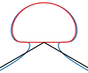
Figure 7 shows comparisons between solutions of the simplified model and the almost self-intersecting solutions obtained from the boundary integral equation method. The black line represents the assumed $120^{\circ }$ angle. To plot these solutions under the same scaling, we enlarge the profiles of the simplified model and then move the profiles vertically so that their top and bottom match the highest point and flat bottom of the bubble structure of the primitive problem. The density ratios from figure 7(a–d) are $0.01$, $0.05$, $0.1$, $0.2$, respectively. It is observed that for a small density ratio, the simplified model provides a good approximation to the almost self-intersecting solution of the primitive equations and further to the limiting configuration shown in figure 1, if it exists.

Figure 7. Comparisons between the almost self-intersecting solutions (blue curves) and profiles resulting from the simplified model (red curves). The black lines represent solid walls intersecting at a $120^{\circ }$ angle. (a) $R=0.01$, (b) $R=0.05$, (c) $R=0.1$, (d) $R=0.2$.

Case II: $\gamma \neq {2{\rm \pi} }/{3}$

It is natural to ask what happens to the reduced model when $\gamma \neq {2{\rm \pi} }/{3}$. In fact, numerical solutions can be found for arbitrary $\gamma \in [0,{\rm \pi} ]$. Four typical solutions with $R = 0.1$ are shown in figure 8.

Figure 8. Solutions of the simplified model for: (a) $\gamma ={{\rm \pi} }/{18}$; (b) $\gamma ={{\rm \pi} }/{3}$; (c) $\gamma ={13{\rm \pi} }/{18}$; (d) $\gamma ={17{\rm \pi} }/{18}$.

Two limiting cases, $\gamma = 0$ and $\gamma = {\rm \pi}$, merit special attention. As can be seen from figure 8, the profile becomes more and more circular as the value of $\gamma$ is decreased. Therefore, one may expect a perfect circular interface to appear when $\gamma = 0$. In fact, it is not difficult to check that $\zeta = \text {i}t(1-t^2)a_0$ is an explicit solution of (4.12), where $a_0 = \sqrt [3]{(1-R)/4R}$. One can then obtain the parametric form of the interface as

(4.14a,b)\begin{equation} x ={-}\frac{1}{4a_0}\sin 2\sigma,\quad y ={-}\frac{1}{4a_0}(\cos 2\sigma-1), \end{equation}

which is a circle with radius ${1}/{4a_0}$. The numerical solution for $R = 0.1$ is plotted in figure 9, where the profile and streamlines are displayed in panel (a) while the comparison with the exact solution is in panel (b). It thus demonstrates the validity of the numerical algorithm.

Figure 9. (a) Numerical solution for $\gamma = 0$ and $\mu = {{\rm \pi} }/{2}$ (solid curve) and streamlines (dashed curves). (b) Comparison between the numerical solution (solid curve) and theoretical prediction (red circles).

For the case of $\gamma = {\rm \pi}$, the bottom of the fluid bubble entirely attaches to the solid wall, therefore the interface should intersect the solid wall with a $120^{\circ }$ angle and form a stagnation point according to the local analysis. A typical solution for $R=0.1$ is shown in figure 10 by setting $\mu = {2{\rm \pi} }/{3}$ and dropping equation (4.11) because the profile is no longer closed at the origin. This type of solution, which describes a still water bubble lying on the flat bottom, exists for all $R\in (0,1)$ owing to the geometrical similarity (4.13a,b). Unlike those shown in figure 6 that represent the limiting solutions for $R\ll 1$, the profile shown in figure 10 corresponds to another possible limiting configuration of interfacial solitary waves, which appears under the Boussinesq limit, i.e. $R\to 1$. Such solutions were found by Pullin & Grimshaw (Reference Pullin and Grimshaw1988) when the upper fluid is infinitely deep. They proposed that in such a scenario solitary waves are unbounded, and calculated the limiting configuration by fixing the wave height and gradually decreasing the lower layer thickness to zero. In particular, they concluded that the limiting interface features a half-lens shape with an approximate aspect ratio (i.e. the ratio of width to height) of $4.36$, which perfectly agrees with $4.353$ resulting from our simplified model.

Figure 10. Numerical solution for $\gamma = {\rm \pi}$ and $\mu = {2{\rm \pi} }/{3}$ (solid curve), together with streamlines (dashed curves).

5. Concluding remarks

In conclusion, we have found numerical evidence for a possible limiting configuration of interfacial solitary waves. Overhanging solutions which become almost self-intersecting have been calculated via a boundary integral equation method for various density ratios, strongly suggesting a limiting configuration characterised by a stagnation point at a $120^{\circ }$ angle and a closed fluid bubble on top of the angle (see figure 1). A simplified model based on these numerical results has been proposed to study the local structure of these singular solutions. Using a series truncation method, we have found exotic solutions depending on the value of $\gamma$, i.e. the angle formed by two intersecting walls. When $\gamma = {2{\rm \pi} }/{3}$, the simplified model provides a good approximation to those almost self-intersecting solutions for small density ratios. Solutions for other values of $\gamma$ have also been computed. In particular, we have found an explicit solution featuring a circular profile for $\gamma = 0$, and a solution corresponding to another limiting configuration of interfacial solitary waves for $\gamma = {\rm \pi}$. Furthermore, it is important to mention that the reduced model can also be applied to periodic interfacial waves owing to its local nature. Finally, considering the crest instability of the Stokes highest waves (see detailed numerical investigations by Longuet-Higgins & Tanaka Reference Longuet-Higgins and Tanaka1997), the Kelvin–Helmholtz instability of interfacial gravity waves (Benjamin & Bridges Reference Benjamin and Bridges1997) and the Rayleigh–Taylor instability owing to the mushroom structure, it is very likely that the almost limiting configurations of progressive interfacial waves are unstable. Therefore, the competition mechanism among different instabilities and the time-evolution of the instability are of particular interest which merit further thorough studies. The only paper we know that provides stability results for interfacial solitary waves is the paper of Kataoka (Reference Kataoka2006). For small amplitude solitary waves, linear stability analyses based on the Korteweg–de Vries (KdV) equation and its modified version (mKdV equation) show that these waves are stable. Using an asymptotic analysis, Kataoka (Reference Kataoka2006) constructed a general criterion for the stability of interfacial solitary waves with respect to disturbances that are stationary relative to the basic wave. Interesting results were obtained for small density ratios. In particular, table 1 in the paper of Kataoka (Reference Kataoka2006) provides critical wave amplitudes $H$ at which an exchange of stability first occurs for air–water solitary waves ($R=0.0013$) with various depth ratios $h$. According to this table, all the waves considered in the present paper are unstable. However, the mechanism of the instability is of great interest, because it is related to the theory of wave breaking. As said above, it was suggested that the instability of solitary waves is caused by the crest instability. Assuming that the local crest instability is also the correct mechanism of interfacial solitary wave instability, there is still one important question. Kataoka (Reference Kataoka2006) found that the exchange of stability occurs at the extremum in the total wave energy. What is the physical connection between the crest instability, which is a local phenomenon, and the extremum in the total wave energy, which is a global quantity? On an apparently completely different problem related to super free fall, Villermaux & Pomeau (Reference Villermaux and Pomeau2010) commented on the formation of a concentrated ‘nipple’ on top of an essentially flat base solution and wondered about the relevance to wave breaking. They noted that wave breaking does occur with standing waves (Taylor Reference Taylor1953) and in nature. The formation of ‘nipples’ can easily be observed on wave crests. These nipples then bend and splash on the sea surface, which forms foam and spume. Is the present study definitely irrelevant to that common but yet unexplained phenomenon? We believe that some interesting dynamics arising from the instability of interfacial solitary waves at small density ratios is likely to occur.