1. Introduction
Natural disasters are likely to be harmful for economic activity. Disasters often cause many deaths, which, apart from personal tragedies, imply a loss of human and intangible capital. Moreover, natural disasters destroy parts of the physical capital stock, such as infrastructure, housing or factories, causing a loss in productive capacities, which may result in short-term and long-term income losses.
Many studies deal with the effect of natural disasters on economic development. Although one might intuitively expect a negative effect of disasters on development and growth, the results of early studies are quite ambiguous and depend on country samples, data, and estimation methods. Early cross country studies consider data on insured damages or the death toll to measure the intensity of natural disasters (see, e.g., Kahn, Reference Kahn2005; Loayza et al., Reference Loayza, Olaberria, Rigolini and Christiaensen2012). The methodological problem is that the data on the disasters is highly endogenous, since income and growth themselves determine the degree of insurance or the number of deaths (Toya and Skidmore, Reference Toya and Skidmore2007). Therefore, more recent studies such as Strobl (Reference Strobl2012) and Felbermayr and Gröschl (Reference Felbermayr and Gröschl2014) measure events and intensities with exogenous geophysical or meteorological information, such as the Richter scale or wind speed. These studies find a negative impact of disasters on country level growth rates. In Barone and Mocetti (Reference Barone and Mocetti2014) and Felbermayr and Gröschl (Reference Felbermayr and Gröschl2014), the effects differ between countries depending on income and institutions. High income countries and democracies show no significant negative effects of disasters, while the opposite is true for low and middle income countries with poor institutions. However, it is still questionable whether there are no negative effects in highly developed countries. Those countries might just go into debt to finance reconstruction because of their better access to capital markets. But still the money spent on reconstruction will be missing elsewhere and thus the disaster affects growth prospects as well.
One reason for the inconclusiveness of existing studies could be that the aggregation of income data at national levels averages out the effects of natural disasters at the regional level. In the earthquake setting, a disaster of a given intensity on the Richter scale in a small country such as Haiti may have completely different effects on national growth compared to a large country such as the USA. In order to deal with this issue, the literature usually scales disaster intensities by the overall land area (Skidmore and Toya, Reference Skidmore and Toya2002). However, given the internal geographical heterogeneity of countries in terms of terrain, weather conditions, and soil quality, which in turn cause differences in the population distribution and therefore the potential number of affected people, this approach may be judged to be rather crude. Therefore, the consideration of exact geographical data might increase accuracy and explanatory power. For example, Haddad and Teixeira (Reference Haddad and Teixeira2015) use the exact positions of floods in São Paulo to identify affected firms and infrastructure in order to analyze the damage. We contribute to the literature by adopting this approach to earthquakes, extending the analysis to all countries in the world.
Our main innovation is that we study the effects of earthquakes at the regional level, i.e., based on grid-cells. For this purpose, we combine geocoded physical event data on earthquakes with geocoded satellite nighttime light data. Recent studies, such as Chen and Nordhaus (Reference Chen and Nordhaus2011) and Henderson et al. (Reference Henderson, Storeygard and Weil2012), demonstrate that nighttime lights are a suitable proxy for income and growth at the country level. Other researchers, such as Hodler and Raschky (Reference Hodler and Raschky2014), Alesina et al. (Reference Alesina, Michalopoulos and Papaioannou2016), Henderson et al. (Reference Henderson, Squires, Storeygard and Weil2017), and Lessmann and Seidel (Reference Lessmann and Seidel2017), use the data to measure income and income differentials at the regional level. Overall the studies find that light is a suitable proxy for regional development. Raschky (Reference Raschky2013) is the first study that uses luminosity data in order to analyze the regional effects of the earthquake in West Sumatra in 2009. Based on a regression discontinuity design, he finds that insurance schemes positively affect recovery rates. Closely related to our work is Klomp (Reference Klomp2016) who also combines nighttime lights as a proxy for economic activity with data on natural disasters. The intensity of geophysical events is measured through the EM-DAT data base using information on fatalities, injuries, etc. and he aggregates all variables at the country level. He finds a positive effect of geophysical events on growth in luminosity that is attributed to recovery investments. We depart from this study by focusing on the regional level (grids) and by using geophysical data on the exact position and intensity of earthquakes. A recent study by Felbermayr et al. (Reference Felbermayr, Gröschl, Sanders, Schippers and Steinwachs2018) also uses night lights combined with geophysical event data on natural disasters. They find negative effects of extreme weather (storms, precipitation, droughts, and cold) but disregard earthquakes, which are our focus.
In our analysis, we exploit several advantages that night light data have over (regional) income data. First of all, this physical data is available for all countries and regions of the world. In particular, in developing countries, there is a lack of capacities in statistical authorities, therefore national accounts suffer from serious measurement errors and regional data is often completely unavailable. Excluding those countries from the analysis might cause a serious selection bias and yield misleading conclusions on the effects of natural disasters. Second, the night light data is available on a grid of approximately 1 × 1 km2. This allows us to analyze the effects of earthquakes at various spatial units without being bound by any administrative or national border. This is particularly important given that regional economic accounts are based on administrative regions, which are very heterogeneous in terms of size. Moreover, boundaries may be endogenous to income. The night light data allows us to consider grids at different resolutions, which are homogeneous by construction.
Our approach extends the existing literature in several dimensions. First, using geocoded physical data for both the dependent and the independent variables offers highly objective data. Second, we get a full picture of the world and probably reduce a potential selection bias in the estimates of previous studies. Third, the approach of using physical event data allows us to use the full earthquake information on epicenter, intensity, location and intensity of aftershocks. In contrast to other studies that focus on the Richter scale to measure an earthquake's intensity at the country level (e.g., Felbermayr and Gröschl, Reference Felbermayr and Gröschl2014), we distribute the incoming seismic energy of an event and all its aftershocks in space. We use the exact position of the epicenter and the radius in which damages are likely to appear to construct potential damage areas for each single event in a fine grid of 0.01° × 0.01° degrees. Our approach allows damage areas of different shocks to intersect. Based on this, we aggregate the incoming energy of different events and distribute it across larger units. Fourth, we consider national institutions and economic conditions as potential moderating factors (Barone and Mocetti, Reference Barone and Mocetti2014).
Our original data set is based on more than 700 million satellite-year observations for night lights, and the earthquake data distributed by the US Geological Survey covers more than 360,000 events for the considered years (1992–2013). We aggregate data on different spatial levels: a 1° × 1° grid, a 2° × 2° grid, and the country level, which yields final data sets of about 185,000, 70,000, and 3,000 unit-year observations, respectively. Applying panel fixed effects regressions, we find a highly significant negative impact of earthquakes on both night light emissions and light growth rates. Effects are quite large at the local level. An earthquake of 8.0 on the Richter scale reduces light intensity by 2.5 per cent in grid cells of size 1° × 1°. The effects are persistent for about 5 years. The rougher grid and country level data show smaller and less robust effects. Good national institutions, a high income level, a larger government and high saving rates reduce the negative effects of earthquakes in support of Barone and Mocetti (Reference Barone and Mocetti2014) and Felbermayr and Gröschl (Reference Felbermayr and Gröschl2014).
The remainder of the paper is organized as follows. Section 2 explains our data and methodology. The crucial point of our analysis is the measurement of an earthquake's intensity and the distribution of the energy across grid cells. Section 3 explains two different econometric models and presents the estimation results on different grid sizes and the country level. Section 4 sums up and concludes.
2. Data
2.1 Nighttime lights
The literature has recently started to focus on satellite nighttime lights data as a proxy for economic development. See, for example, Elvidge et al. (Reference Elvidge, Baugh, Kihn, Kroehl, Davis and Davis1997) and Henderson et al. (Reference Henderson, Storeygard and Weil2012) at the country level, Chen and Nordhaus (Reference Chen and Nordhaus2011) and Henderson et al. (Reference Henderson, Squires, Storeygard and Weil2017) on the grid level or Lessmann and Seidel (Reference Lessmann and Seidel2017) on the level of sub-national administrative units. The major advantage of nighttime lights over national or regional account data is that it covers the whole world at a high resolution of about 1 km2. Given the high resolution of the data, it can be aggregated at different spatial levels, e.g., grids, administrative units, ethnic groups. We refer to the stable lights product distributed by the National Oceanic and Atmospheric Administration. Please see the overview by Donaldson and Storeygard (Reference Donaldson and Storeygard2016) for the properties of the data.
In economic geography, the ‘modifiable areal unit problem’ (or MAUP) deals with two important space-related features: (a) the borders are drawn in different ways (zoning), and (b) the size of spatial units varies (scaling) (see, e.g., Openshaw and Taylor, Reference Openshaw, Taylor and Wrigley1979). These heterogeneities may affect econometric results significantly, therefore it is important to study the relationship between disasters and economic outcomes at different spatial levels.
Following Henderson et al. (Reference Henderson, Squires, Storeygard and Weil2017), we aggregate nighttime lights at a 1° × 1° grid, but we also take a broader perspective considering a 2° × 2° grid. In the fine grid, a unit of observation has the size of approximately 110 × 110 km2, which corresponds to the size of the U.S. state of Connecticut or approximately a 1/800 part of total U.S. land mass. For each cell, we build the sum of lights, i.e., the sum of digital number (DN) values of all inherent pixels. We also compare the grid cell level regressions with outcomes at the national level using data from the Global Administrative Areas Project (GADM). The forthcoming panel fixed effects regressions use the log sum of lights and light growth rates as dependent variables, alternatively.
In our particular context, a discussion is needed as to whether light emissions are a suitable proxy for economic activity in the aftermath of an earthquake. Most stable light emissions are caused by street lights, light emissions of buildings and industrial facilities. These emissions require access to the power grid that is often disconnected following a natural disaster. Naturally, most man-made light emissions cannot emerge without electricity. The question arises of whether we measure only short-run effects caused by an interrupted access to electricity, or a medium- or long-run effect on economic activity.
Access to the power grid is not the most serious bottleneck for economic activity in the aftermath of an earthquake. In highly developed countries, the power supply is quickly restored even after large events. Liu et al. (Reference Liu, Nair, Lopez Renton and Wilson2017) show that, for an earthquake in New Zealand of magnitude 7.8 in 2016, the power grid connections were restored within 24 hours. Kammouh et al. (Reference Kammouh, Zamani Noori, Marasco and Cimellaro2018) estimate restoration curves for both developed and developing countries, finding that the power system is restored with a probability of close to 100 per cent within 60 days right after the event. Note that it takes significantly longer to restore water, gas and telecommunication systems. Therefore, the partial effect of a disaster on night lights coming just from missing electricity for unproductive light emitters like street lights tends to be rather small. In the empirical analysis, we deal with this issue in two ways. First, in addition to contemporary values of the event variable, we consider several time lags. This allows us to investigate the change in night lights that is not caused simply by a temporary disconnection to the power grid. Second, we provide robustness tests where we include the country level rate of access to electricity as a control variable in order to capture parts of the effects related to missing electricity.
One issue we cannot resolve with the night light data is the weak relationship between light and income in rural, sparsely populated areas (Keola et al., Reference Keola, Andersson and Hall2015). Earthquakes have a lower seismic risk in rural compared with urban areas, since there is a lower concentration of vulnerable structures and complex functions. Nevertheless, earthquakes harm the people living in remote villages and there is an additional risk of isolation that delays disaster relief and reconstruction. Given that the rural economic activity is not well reflected in our light data, we cannot derive any conclusions about the effects of disasters here. Our analysis is more representative for regions with a higher population density and a relatively high share of gross value added in manufacturing and services. Rural regions with a high share of agriculture – that happen to be dark in the satellite images anyway – are not appropriately covered by our approach.
Finally, we discuss alternative data which might be used as the outcome variable instead of night lights. There are mainly two alternatives: the Geographically based Economic data (Nordhaus and Chen, Reference Nordhaus and Chen2016) and regional economic accounts provided by national statistics and international organisations that have been used by Gennaioli et al. (Reference Gennaioli, La Porta, Lopez De Silanes and Shleifer2014), Lessmann (Reference Lessmann2014), and others. The G-Econ data provides gross cell output on a 1° × 1° grid in four waves (1990, 1995, 2000, 2005). The data combines regional GDP estimates with gridded population data. Under the assumption that output is equally distributed within sub-national administrative regions, the population data is used to distribute GDP across grid cells. Note that GDP data for the lowest available sub-national division is used, which is – in many developing countries – the national level itself. In this case, the population distribution is the main driver of gross cell output. For our purposes, this data set has some disadvantages which is why we prefer night lights. First, the frequency and period coverage is not as rich as in the night lights data. Given that we expect different effects of earthquakes in the short-, medium-, and long-term perspective, we need the high variation in the annual data. Second, while we have to decide in the annual data what share of an earthquake's energy happening in a certain month has to be shifted to the following year, the decision becomes quite sensitive when using data in waves with 4-year gaps. Third, GDP based regional data often has a low quality in less developed countries for reasons of low capacity of statistical offices (Chen and Nordhaus, Reference Chen and Nordhaus2011) or due to strategic misreporting (Martinez, Reference Martinez2019). Moreover, in the aftermath of a disaster, GDP estimates are highly uncertain and output data revisions are frequent, in particular in developing countries (Ley and Misch, Reference Ley and Misch2014). Therefore, we prefer night lights over GDP based data, since night lights are objectively measured and comparable across countries, even in times of crisis. However, as a robustness check, we present regressions using population as a dependent variable, which is the main determinant of gridded output in the G-ECON data for developing countries.
2.2 Earthquakes
Data on earthquakes are reported by the U.S. Geological Survey. The data include the exact date, location at a resolution of 0.001°, and magnitude of every earthquake. During our observation period from 1992 to 2013, which is limited by the availability of the luminosity data, the geoscientists recorded 364,317 earthquakes, whose range per year varies between 6,733 and 26,016 without systematic trend. The countries with the largest number of earthquakes are the USA (19,774), Chile (12,383), and Mexico (8,299). The strongest events inside a country have been recorded in Indonesia with magnitude 8.2. The strongest two events were measured with magnitude 9.0. One was near the east cost of Japan in March 2011, causing the Fukushima nuclear accident; the other one was off the northern west coast of Sumatra in December 2004, with more than 250,000 deaths in 14 countries. Note that these examples imply that it is important to distribute the earthquake energy in space. Although the epicenter may be located far away from economically active regions, there might still be effects on those, in particular, if the epicenter is offshore.
We transform the raw data on earthquakes in different non-trivial ways. Our major aim is to measure the exact energy of an earthquake and its aftershocks received by one cell. Different approaches are possible. The easiest, but rather crude one, would be to consider only the strongest event and to use its magnitude on the Richter scale. However, this is naive for different reasons. This approach ignores the exact position of an earthquake within a cell and the reasonable destruction caused by aftershocks and their timing. One single, relatively large event might be less harmful than a sequence of slightly smaller events. For example, the earthquake in Morocco on February 24th, 2004 with a magnitude of 6.4 had 164 recorded aftershocks in just 24 hours; the strongest aftershock had a magnitude of 5.3 which also has a relevant destructive power and, of course, its own epicenter. Note that aftershocks are often the cause of the collapse of previously damaged buildings. There are also countries such as Greece which are hit by many earthquakes of similar size in one year. For example, the Greek island of Zakynthos was hit by one earthquake with magnitude 5.7, three with magnitude 5.5 and one with magnitude 5.4 in the year 2006. In these cases, considering only the event with the highest magnitude does not appropriately reflect the total destructive energy of earthquakes and their distribution across regions. Therefore, it is necessary to develop a new methodology which allows us to combine several earthquakes and to take into account their exact location within a cell.
In order to distribute the physical energy of an earthquake and its aftershocks within and across cells, we create a very fine grid of 0.01° × 0.01°. Based on this fine grid, we calculate the incoming physical power for each cell depending on the distance to the epicenter and the magnitude of the event. Geoscience AustraliaFootnote 1 provides estimations of the damage radius for every magnitude. An earthquake of magnitude 9 on the Richter scale has a damage radius of approximately 735 km, while a weaker event with a magnitude of 6 has a damage radius of 37 km. Based on this information, we draw circles around each epicenter and distribute the energy linearly decreasing in the distance of a cell to the epicenter.
Another important issue we have to take into account is that the Richter scale does not measure the intensity of an earthquake on a linear scale, but on a common logarithmic basis for the amplitude of waves recorded by seismographs. Thus, a one-unit increase in magnitude is associated with a tenfold increase in measured amplitude and about 30 times more seismic energy (Spence et al., Reference Spence, Sipkin and Choy1989). Consequently, a linear interpretation of the Richter scale is inappropriate in this matter.
Figure 1 illustrates our approach. Panel (a) is a 3D plot with earthquake intensity on the vertical axis; panel (b) is a bird's eye view of the distribution of the earthquake intensity in space. The epicenter cell gets the value 10M, where M is the reported magnitude on the Richter scale. The radius of the cone is determined by the damage coverage estimates reported by Geoscience Australia. In our illustrative example, we refer to three hypothetical events with magnitudes of 6.0, 6.6 and 7.0. The radius of the event with magnitude 6.0 is 37 km, which corresponds to about 0.3° at the equator. The epicenter pixel of this event receives a value of 106 as a measure of the earthquake's maximum intensity. The values of the other pixels decrease linearly with the distance to the epicenter until the value is zero at the border of the circle. Analogously we construct the two other events. Based on these three intersecting events, we sum up the energy from the distinct events for each cell in the fine 0.01° × 0.01° grid which is hit by more than one shock. Note that this method of aggregation would have been meaningless using the original Richter scale data. Panel (b) shows a 2D plot for this example where different values are expressed by different colors.
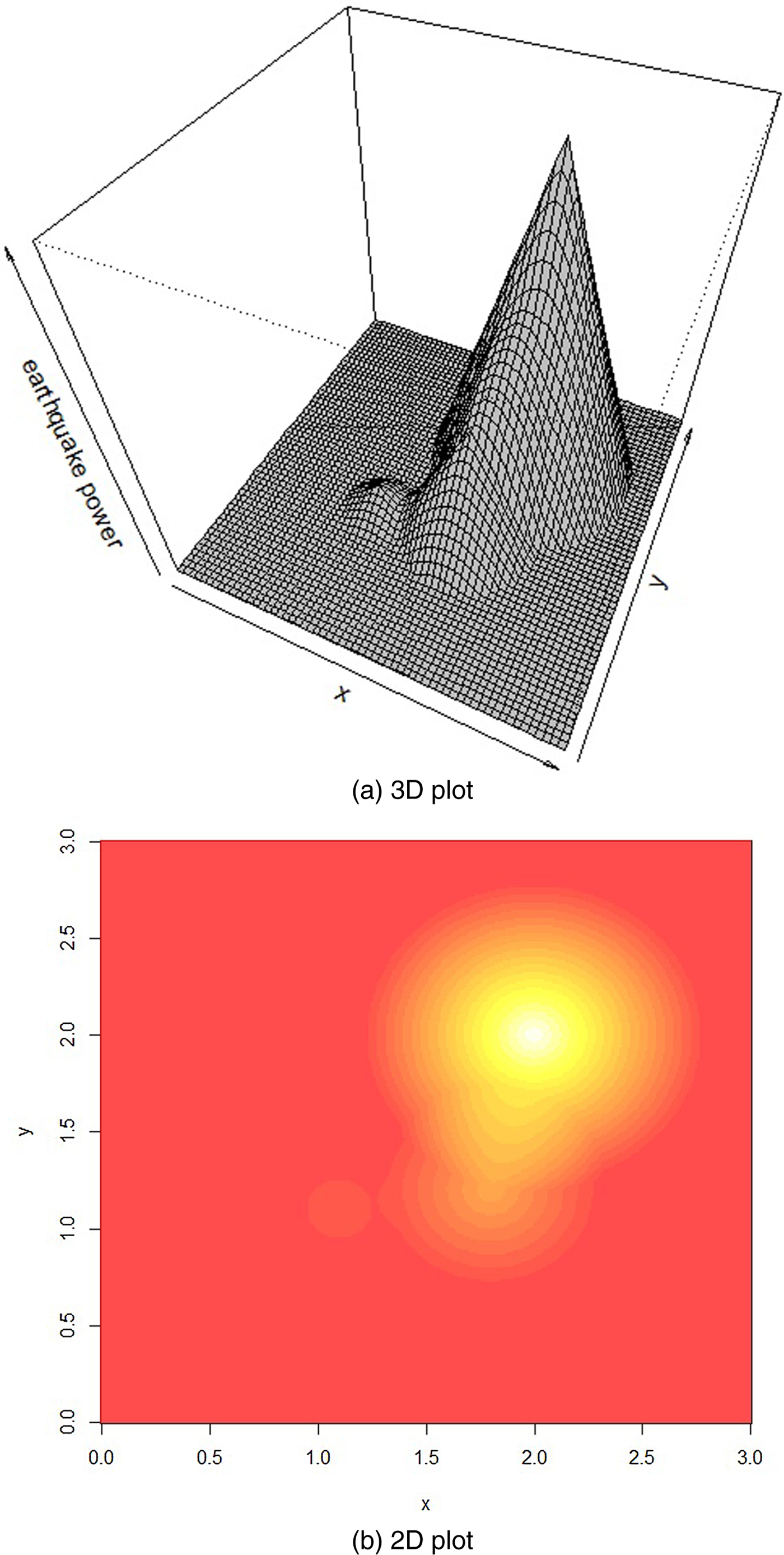
Figure 1. Incoming seismic energy in space.
Our approach has two major advantages. First, if there are many earthquakes in one region whose damage radii intersect, we can simply sum up the calculated energy at the grid level. Second, if an earthquake affects more than one region on the rougher 1° × 1° that we use in our econometric models as the main unit of observation, we can distribute the damage across the different units according to the energy values we compute at the fine 0.01° × 0.01° grid.
This new feature is illustrated in figure 2. The map shows two big earthquakes and their aftershocks which took place in Peru and Chile in 2007. The epicenter of the Tocopilla earthquake was located between the localities of Quillagua and Tocopilla, affecting the Tarapacá and the Antofagasta regions in northern Chile. The earthquake had a moment magnitude of 7.7 and was followed by a number of strong aftershocks with a magnitude of up to 7.1. The earthquake in Peru had a magnitude of 8.0 and affected the Ica region. Aftershocks were recorded with a magnitude of up to 5.9.
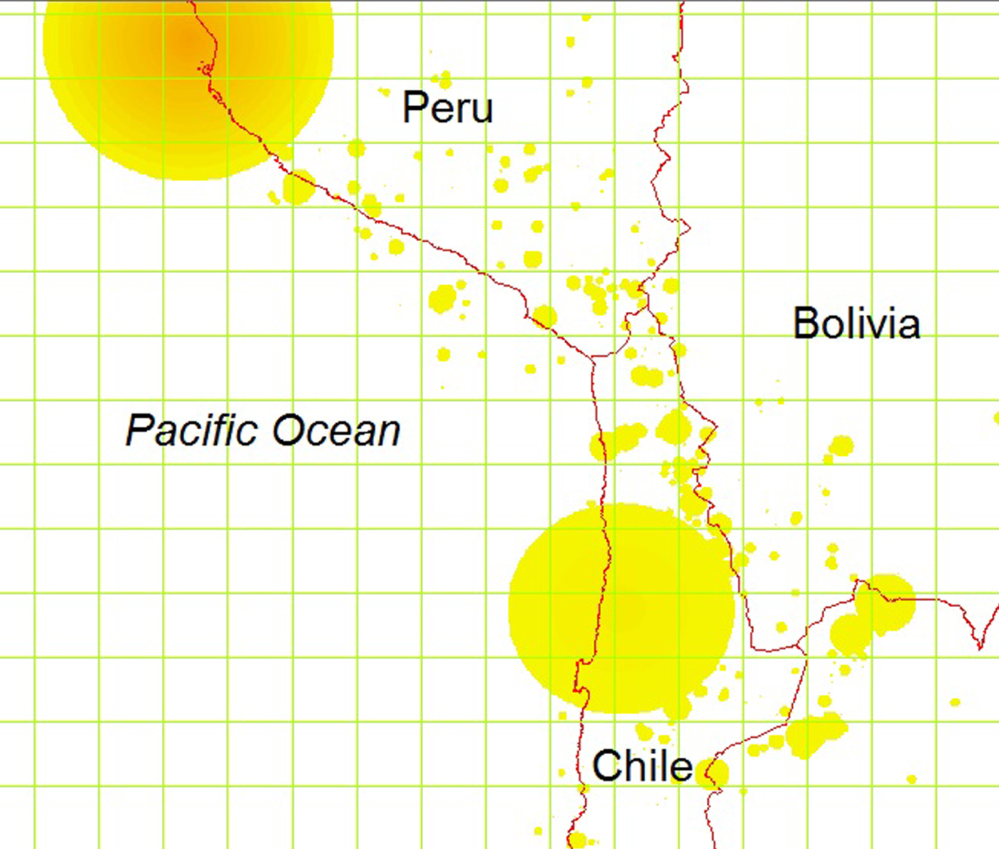
Figure 2. Analyzing earthquake impact with grids.
The green grid lines reflect the 1° × 1° grid we use to study the impact of earthquakes on night lights. The circles are the damage areas of the earthquakes where the radius depends on the magnitude. We choose the colors within the circles according to the magnitude of the earthquake as discussed above and distribute the energy across the area according to the distance to the epicenter. Considering the case of Peru, the highest magnitude in the epicenter is dark orange and energy decreases linearly with the distance to this location from light orange to yellow (cooling down effect).
Obviously, an earthquake is first and foremost a local shock, therefore is seems to be somewhat misleading to study the effects at the country level as is common in the literature. However, looking only at the epicenter would also be problematic, given that damages also occur in neighboring cells. Taking the earthquake in Chile as an example, we can simply consider the cells which are affected. Disregarding grid cells over water, we find that twelve grid cells are in the damage area. Therefore, our methodology allows us to distribute the energy of an earthquake across space, which is a new feature in the literature.
A final aspect that has to taken into account is the exact date of an earthquake. The satellite night light data report annual-average luminosity values of cloud-free evenings. It is obvious that an earthquake in January has a different effect on the average light intensity in a year compared with an earthquake in October. To deal with this issue, we follow the time correction method suggested by Klomp (Reference Klomp2016). If, for example, an earthquake happens in May 2004, we will split the event's energy and move 7/12 and 5/12 to the corresponding 2004 and 2005 values, respectively.
Note that we apply a simple scaling to the final energy values at the grid cell level. Since we aggregate energy values of the fine 0.01° × 0.01° grid, the maximum of energy assigned to a 1° × 1° grid cell is of order 1E13.Footnote 2 Consequently, the coefficients in our forthcoming regression analysis would be very small. For reasons of exposition, we divide all values by 1013. Please see table A1 in the appendix for descriptive statistics of all variables considered in our analysis.
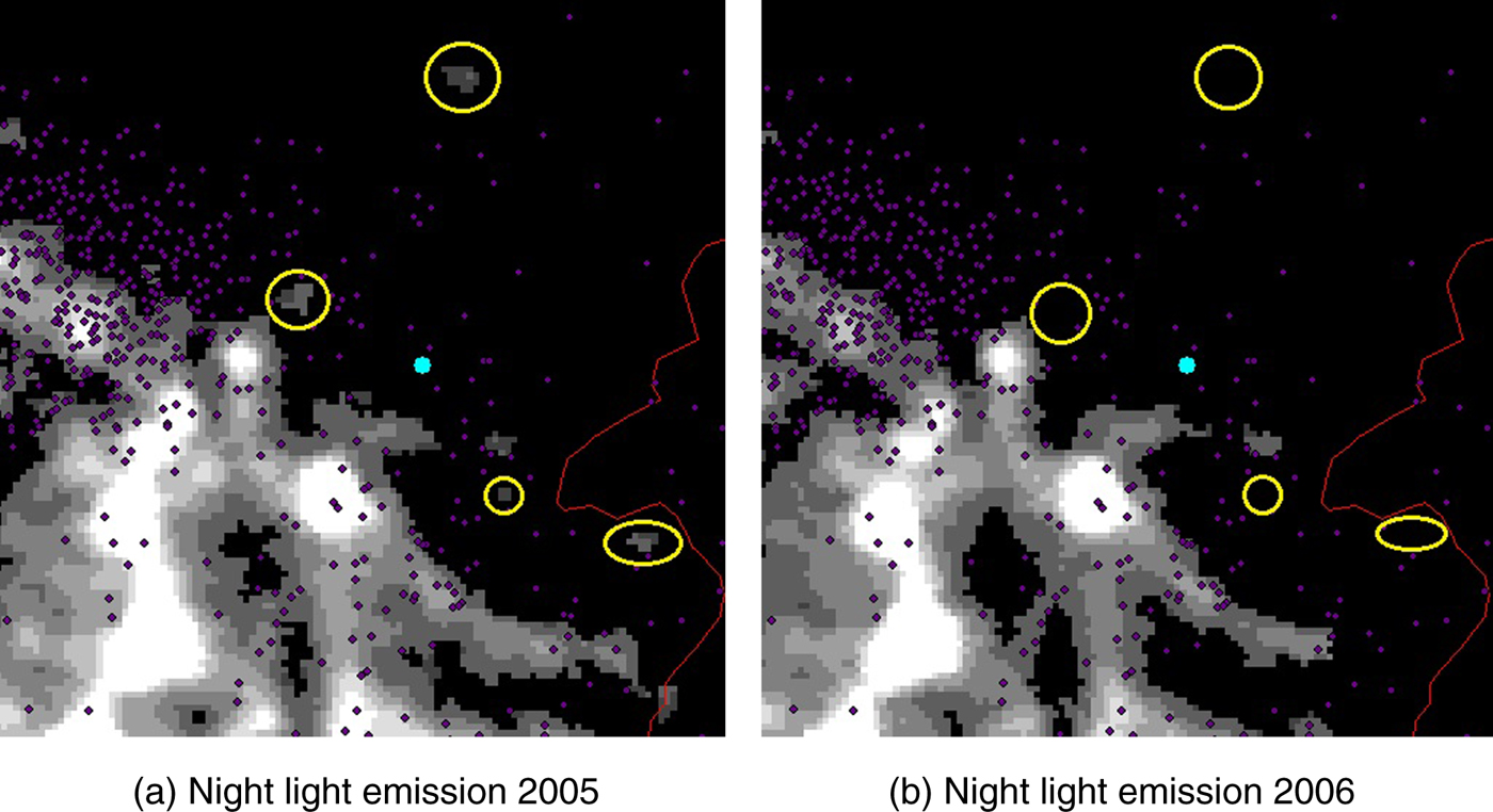
2.3 The case of Pakistan 2005/2006
Before we move to the main analysis, we do some eyeball econometrics on the relationship between earthquakes and night lights. Figure 3 shows satellite pictures of the northern part of Pakistan. The region was hit by an earthquake of magnitude 7.6 on October 8th, 2005 and resulted in 73,000 victims on Pakistani territory.

Figure 3. Earthquake northern Pakistan in 2005.
Panel (a) shows the average light intensity in 2005, and panel (b) for the subsequent year. The blue point is the epicenter of the main event and the purple points are the aftershocks. We observe a strong reduction in night light emissions in the affected areas, especially inside the yellow circles. A village in the north of the epicenter is completely unlit one year after the shock. Also in the northwestern parts of the region, the luminosity decreased significantly. To analyze the differences in light emissions between 2005 and 2006, we construct a 1° × 1° rectangle with the epicenter in the middle of the cell. Our data shows a decrease of 6.6 per cent in total luminosity.Footnote 3 This corresponds to estimations on damages. The total costs of reconstruction were calculated at US$3.5 billion, of which US$416 million were needed to reconstruct transport infrastructure including roads and bridges.Footnote 4
3. Estimation results
3.1 Empirical framework
In this section, we estimate the impact of earthquake intensity on satellite night lights. We concentrate on a fine 1° × 1° grid and a rough 2° × 2° grid. We also compare the outcomes with country level aggregates. The fine grid has potentially 64,800 cells. Following Henderson et al. (Reference Henderson, Storeygard and Weil2012), we focus on regions between 65 degree south and 75 degrees north latitude, which reduces the data set to 50,400 cells. Next, we remove all cells that are completely dark and uninhabited (in particular cells over water), which yields our final data set of 8,839 cells, which we study over the sample period from 1992–2013. The amount of considered 2° × 2° cells is 3,177. Our data set considers 190 countries in total.
Our econometric analysis has to take three important issues into account: (1) unobserved heterogeneity, (2) spatial dependency, and (3) satellite configuration. Ad (1) Our unit of observation is homogeneous in terms of size, but heterogeneous in terms of other characteristics such as geography and climate. By using grid-cell fixed effects, we take observable and unobservable time-invariant heterogeneities into account. Ad (2) The economic activity, i.e., the light-intensity within one cell, depends on the conditions in surrounding cells. Low- and high-output density regions are clustered in space, which has to be taken into account, in particular if fine grids are studied. We therefore consider the sum of light values in the eight directly neighboring cells as a spatial control variable to account for the spatial spillover effects. Ad (3) The satellite configuration and sensor technology changes over time and sensors degenerate during its typical 5-year activity period. Thus, we make use of satellite configuration dummy variables in addition to year fixed effects.
Given that each cell is inhabited by a different number of people, we control for the (logarithmic) population. Population data are provided by the Center for International Earth Science Information Network. Since the data is published in 5-year waves, we interpolate missing values in order to get annual data.
The literature makes use of two different general estimation approaches. (1) Some studies consider growth rates as dependent variables and control for initial levels just like in the well-established growth literature (see, e.g., Skidmore and Toya, Reference Skidmore and Toya2002; Noy, Reference Noy2009; Strobl, Reference Strobl2011; Loayza et al., Reference Loayza, Olaberria, Rigolini and Christiaensen2012; Felbermayr and Gröschl, Reference Felbermayr and Gröschl2014). (2) Other studies analyze levels and include lagged dependent variables to account for the inter-temporal dependencies (see, e.g., Raddatz, Reference Raddatz2007; Cavallo et al., Reference Cavallo, Galiani, Noy and Pantano2013; Felbermayr and Gröschl, Reference Felbermayr and Gröschl2013; Klomp, Reference Klomp2016). We apply both approaches in order to be comparable to the different strands of the literature.
(1) Growth model:
In the growth specification, we regress light growth on initial lights, earthquake energy and controls. Our model for N grid cells and T time periods, cells indexed by i and time by t, respectively, has the following form:
 $$\eqalign{\log \left( {\displaystyle{{y_{i,t}} \over {y_{i,t-1}}}} \right) = & \alpha \cdot \log (y_{i,t-1}) + \sum\limits_{j = 0}^2 {\beta _j} \cdot \log (D_{i,t-j}) \cr & + \gamma _1\cdot \log (p_{i,t}) + \gamma _2\cdot \log ({\tilde{y}}_{i,t}) + \delta _t + \mu _t + \alpha _i + u_{i,t},} $$
where y i,t is a grid cell's sum of lights, ỹ i, t is the average light of the neighboring cells, D i,t is the impact energy of earthquakes, p i,t is cell i's population size, δt are time fixed effects, μt are satellite configuration fixed effects, αi are grid cell fixed effects, and u i,t is the error term. For the investigation of countries instead of grids, we aggregate all data from the 1° × 1° grid to the country level and we use country fixed effects instead. Note that we add 1 before applying the logarithmic transformation of the variables in order to eliminate negative values.
(2) Level equation:
As an alternative specification, we regress light levels on (lagged) earthquakes, and controls. The model has the form:
 $$\log (y_{i,t}) = \sum\limits_{j = 0}^4 {\beta _j} \cdot \log (D_{i,t-j}) + \gamma _1\cdot \log (p_{i,t}) + \gamma _2\cdot \log (\tilde{y}_{i,t}) + \delta _t + \mu _t + \alpha _i + u_{i,t}.$$
This specification aims to analyze the mid-term effects of earthquakes, since we can investigate the number of years for which we find significant coefficients of lagged values of disasters' energy.
3.2 Estimation results
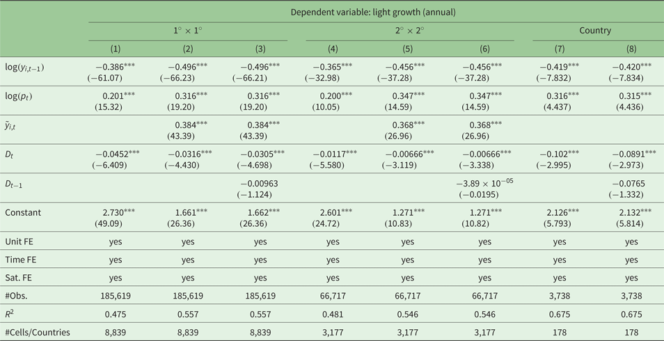
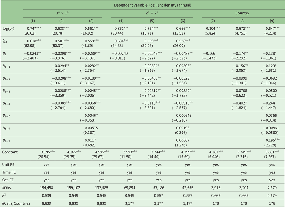
We first turn our attention to the growth model. The regression results are reported in table 1. Columns (1)–(3) report the results we obtain on the fine 1° × 1° grid; columns (4)–(6) report results for the 2° × 2° grid. The last two columns, (7) and (8), report results at the country level. Note that we use the original annual data thereby concentrating on a short-run relationship between the variables of interest.
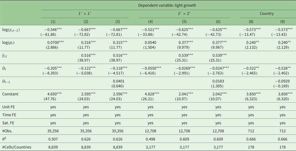
Table 1. Results of the growth model (a) using annual data

Robust t-statistics in parentheses. ***p < 0.01.
Standard errors clustered at the grid cell level and country level, respectively.
We run different specifications of equation (1). Column (1) shows a minimum specification including the initial light level and the population as control variables and, of course, the earthquake energy intensity received by a grid-cell in the contemporary period. Column (2) adds in the light intensity of neighboring cells to account for spatial spillovers. Column (3) adds a one-year lagged value of the earthquake intensity.Footnote 5 We proceed in a similar manner for the regressions on the larger 2° × 2° grid. At the country level, we do not include a spatial lag, therefore we report only two results. We find a strong dependency of the light growth rate on the initial level. The resulting coefficient is negative and highly significant, suggesting strong convergence effects: relatively rich regions – by means of regions with high light emissions – tend to grow more slowly than poor regions. The controls for the population size and the spatial dependency work satisfactorily, as well as having the expected signs: higher population densities increase light emissions, and lights are clustered in space.
The main results concerning the incoming seismic energy are also in line with our expectations. The coefficient of the variable capturing the contemporary effect is negative and highly significant. The size of the coefficient decreases only slightly while including more variables into the model. The lagged values have negative signs but are not statistically significant. Note that we use growth rates as dependent variables and that we control for the initial light level. Effects of prior earthquakes are therefore partially captured by initial light emissions (i.e., log (y i,t−1)).
Regression results based on the 2° × 2° grid are very much in line and show no systematic differences. However, it is important to note that the coefficient of the earthquake variable is significantly smaller in the rough grid compared with the fine grid. This is, again, a quite suggestive result. Earthquakes tend to have more local than supra-regional consequences. Note that we cannot compare the results at the country level with the grid level estimates in quantitative terms due to the data aggregation method. Importantly, in qualitative terms, the coefficients point in similar directions.
Altogether, we conclude that the incoming earthquake energy decreases light growth in affected cells. This should not be interpreted as a similar loss of the capital stock or damage. Lights are a flow figure, which is correlated with current income, production and consumption, in particular if those activities involve electric energy. Current economic activities slow down after an event, but the effect does not have to be persistent.
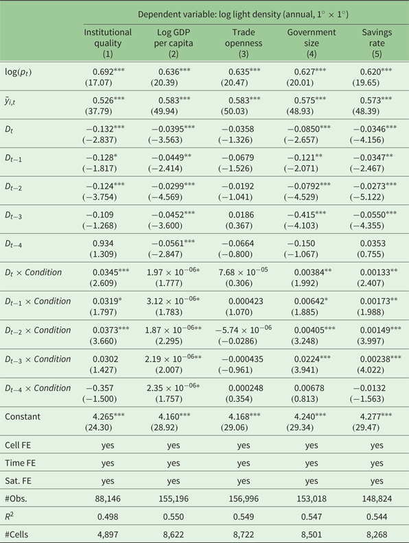
Our second approach explains the within cell variation of log light levels depending on the incoming earthquake energy. The results are reported in table 2. Columns (1)–(3) report the results we obtain on the fine 1° × 1° grid; columns (4)–(6) report results for the rougher 2° × 2° grid; and columns (7)–(9) report country level results.
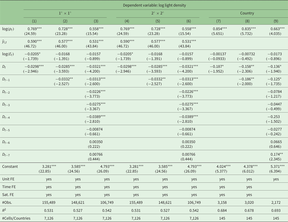
Table 2. Results of the light level model (b) using annual data
Robust t-statistics in parentheses; ***p < 0.01, **p < 0.05, *p < 0.1
Again, we run different specifications of the respective model (c.f. equation (2)). In column (1) we include the population, the light intensity in neighboring cells, and the contemporary earthquake energy. Columns (2) and (3) add lags of the earthquake variable. We proceed in a similar manner for the regressions on the larger 2° × 2° grid and on the country level.
The results support our previous findings. Importantly, we find persistent effects of earthquakes on night light emissions. Not only is the contemporary effect of the earthquake energy negative and significant, but the coefficients of the different lags are as well. Investigating long-term effects – as far as our observation period allows us to do – we find no significant effects after five years. We find interesting and suggestive differences depending on the size of our unit of observation. In the fine 1° × 1° grid, the effects are highly significant for the first five years after an earthquake has happened, even if we consider seven lags. In the rougher 2° × 2° grid, the effects are less significant in statistical terms. Importantly, earthquakes have only short-run effects at the country level. Here, the effect of contemporary earthquakes is not significant. Only by adding some lags does the coefficient become statistically significant, but the results are less robust. Thus, earthquakes are first and foremost a local event. The negative effects on economic activity vanish, the larger the area under consideration is.
Our regressions imply that earthquakes reduce growths rates as well as levels of grid-cell light emissions. However, the coefficients cannot be interpreted easily with respect to the size of the effects. In order to quantify the effects, we consider the fine 1° × 1° grid. We calculate the seismic energy of two hypothetical earthquakes of size 7.5 and 8.0 on the Richter scale, respectively, that hit the grid cell in the centroid on January 1st. The rescaled incoming energy calculated according to subsection 2.2 is approximately 0.023 and 0.084, respectively. Multiplying these energies with the D-coefficient reported in column (1) of table 1, we obtain an absolute reduction of | − 0.0452 · 0.023| = 0.00104 = 0.1% and 0.4%, respectively. If we consider an average grid-cell light growth rate of 5 per cent, the effects are of a relevant order. Given that the regressions of the level model reveal coefficients of similar magnitudes, the effects on the levels of light emissions are of a corresponding size.
3.3 Moderating factors
Next, we explore the role of national institutions and economic conditions on the impact of earthquakes on grid-cell light emissions. We consider the second specification which explains the within grid-cell variation of light levels with (lags of) earthquakes adding sequentially interaction terms of earthquakes and institutional as well as economic variables to equation (2). For this, we follow the general framework of Felbermayr and Gröschl (Reference Felbermayr and Gröschl2014).
Note that we use period averages for the years 2006 to 2013 for the moderating variables instead of annual values. First, this allows us to consider our whole observation period from 1992–2013 for which we do not have balanced information on the moderating factors for all countries in the world. Second, it is likely that the moderators themselves are affected by disasters. For example, the trade-to-GDP ratio declines after a shock (Felbermayr and Gröschl, Reference Felbermayr and Gröschl2013), therefore some part of the variation in the interaction term might come from simultaneous changes in both variables. Using a period average combined with fixed effects restricts the econometric model to exploit only the variation in the earthquake intensity conditional on a fixed value of the moderating variable. Nevertheless, the general level of the conditioning variables might also be affected by the seismic risk (e.g., higher saving rates). Therefore, we do not make a causality claim concerning the effects. The results should be interpreted as correlations.
Table 3 reports the results. We consider an index of institutional quality (column 1), the log of GDP per capita (column 2), a trade openness indicator (column 3), a measure of government size (column 4), and the savings rate (column 5) as conditioning variables.Footnote 6
Table 3. Moderating factors: Interaction models

Robust t-statistics in parentheses; ***p < 0.01, **p < 0.05, *p < 0.1
The results show negative coefficients for the earthquake intensity and its lags, just as in the estimations presented above. Importantly, we find variable interactions to be important in case of institutional quality, development level, government size and savings. The coefficients have positive signs and are statistically significant for at least two lags. Our results are in line with our expectations. Good institutions may accelerate the reconstruction efforts, rich countries are likely to be more resilient to natural disasters, large governments have more budgetary and administrative capacities to manage reconstruction, and high savings allow for more investment after the shock. Trade openness does not turn out to be a relevant moderating factor, although one might expect a positive effect, since open economies have better access to financial markets and imports of investment goods needed for reconstruction.
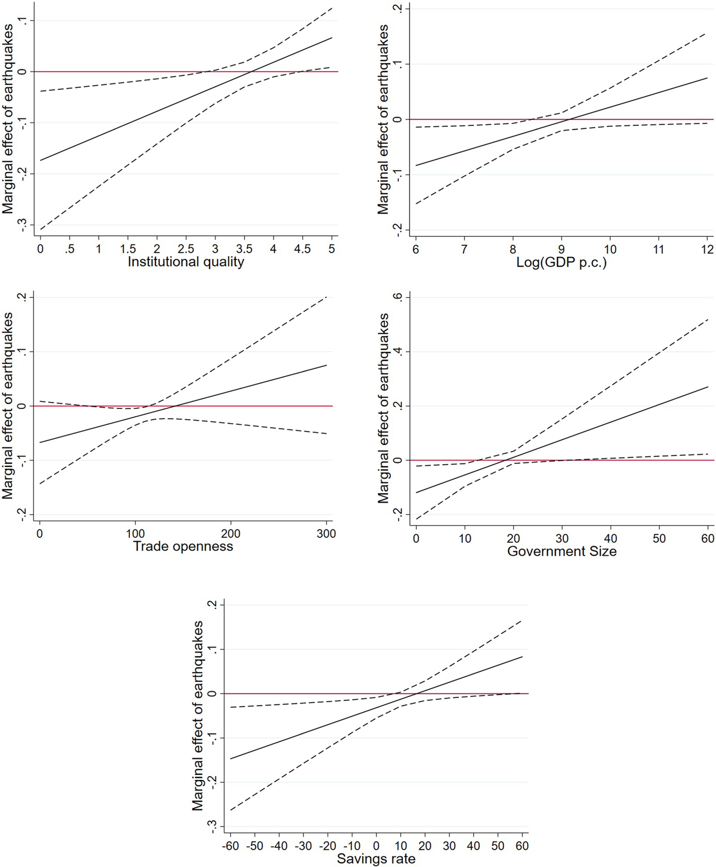
Note that the coefficients of single variables cannot be interpreted properly in interaction models without calculating marginal effects. Even if regression coefficients are significant, this does not necessarily imply that the marginal effects are significant for reasonable values of the conditioning variable. Therefore, we calculate the marginal effects of earthquake energy on grid-cell lights using a reduced specification without lags of variables. Figure 4 illustrates the findings including 95 per cent confidence bands. The results suggest that the effects of earthquakes are only negative in poor institutional or economic settings. Importantly, the effect does not reverse in good settings, where we barely find significant marginal effects.

Figure 4. Marginal effects of moderating factors.
3.4 Robustness tests
In this section, we provide different robustness tests. First, we turn our attention to 5-year period averages instead of annual data in order to shift the focus to a mid-term perspective. Tables A2 and A3 in the appendix present the results of similar specifications to those discussed above. Note that we can investigate only 5 periods, therefore we cannot add a similar amount of lags compared to the estimations using annual data. Concerning the growth model, we find a significant negative effect for both grid sizes. Country level estimates also show negative coefficients, but lower significance levels. In the model that explains changes in light levels, we find significant effects in the small grid for disasters of the same period, but only weak and imprecise effects if we consider the rough grid and the country level.
Second, we include electrification data in our model. As discussed in section 2.1, night light data also captures man-made light emissions that do not directly relate to economic activity (e.g., street lights). Earthquakes disconnect regions from the power grid for up to 60 days, therefore a part of the variation in night lights may be caused just by temporary changes in electrification without a strong effect on output. To tackle this issue at least partially, we include the country level rate of electrification as a control variable. The results are presented in table A4 in the appendix and confirm our main findings.
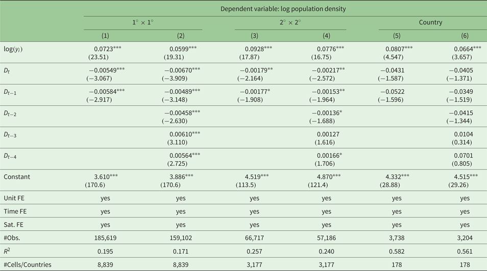
Third, we use the log of the population density as an alternative dependent variable. As mentioned above, the G-Econ data base relies on population raster data in order to distribute output across cells. Population density is a major determinant of night lights and economic activity, since agglomeration indicates favorable geographic and economic conditions. In our robustness test, we run the level model (equation (2)) using output as the dependent variable and (lags) of the earthquake intensity as independent variable(s). The results are reported in table A5 in the appendix. We find highly significant negative effects in the 1° × 1° grid for the contemporaneous earthquake shock and the next two lags. Higher order lags show positive coefficients. The result is in line with our expectations. Earthquakes cause a decrease in population because of fatalities and displacement. However, emigration from affected areas is only temporary and people migrate back once the reconstruction reaches a certain level. The effects are smaller both in terms of size and statistical significance in the rougher 2° × 2° grid, suggesting that the migration distance is limited to surrounding areas. At the country level, these effects vanish completely, implying that displaced persons search for protection predominantly in their home country. Altogether, this supports our main finding that economic activity is significantly negatively affected by earthquakes. It also points to temporary disaster displacement being an important channel.
4. Summary and conclusion
We examine the impact of earthquakes on satellite nighttime lights at the regional level, i.e., based on grids. Our approach extends the existing literature on the effect of natural disasters on economic development in several dimensions.
First, by using satellite nighttime lights as an indicator of economic development, we are able to study almost all regions of the world. Studying the full population of countries instead of particular samples helps to avoid a potential sample selection bias. Second, the satellite nighttime light data can be aggregated at different territorial levels. Therefore, we bring the discussion on the effects of natural disasters to the regional level, thereby focusing on artificially drawn grids of different sizes. We also compare the results with regressions at the country level. Third, we follow recent literature by using geophysical event data on the intensity of earthquakes instead of reported damages. This strategy has the advantage that the size of the shock can be treated as exogenous to the income. Using geophysical event data is, however, not a trivial task in our framework. We therefore develop a new method that allows us to distribute the seismic energy of an earthquake in space and time. Our approach is much more accurate compared to others that, e.g., simply divide earthquake magnitudes by a country's surface. Fourth, we consider national institutions and economic conditions as potential moderating factors.
Our calculations provide a new data set on the earthquake energy received at the regional (grid) level and corresponding satellite nighttime lights. Considering the 1° × 1° grid, the final data set contains 8,839 regions for the period 1992–2013. Based on this new data set, we estimate the effect of earthquakes on lights using panel fixed effects regressions and find a significant negative effect. The effects are also significant in economic terms. An earthquake of magnitude 8.0 reduces light's growth rate by approximately 0.4 per cent. Importantly, space matters in this context, too. The effect is significantly smaller considering a rougher grid or the country level. Earthquakes are, therefore, first and foremost a regional event, which should also be studied at the regional level. Concerning national institutions and economic conditions, we find that good institutions and economic conditions alleviate the negative effects of earthquakes.
Acknowledgments
This research was supported by the German Research Foundation (grant BL1502/1-1). We would like to thank the participants of the lunchtime seminar at the University of Hamburg 2018 for helpful comments.
Appendix
Table A1. Descriptive statistics
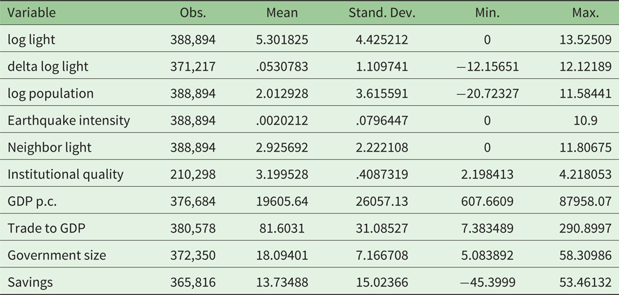
Table A2. Robustness: results of the growth model (a) using 5-year period averages

Table A3. Robustness: results of the light level model (b) using 5-year period averages
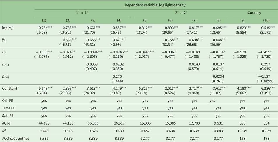
Table A4. Robustness: results light level model (b) including electrification rates (log(E t))

Table A5. Robustness: population density as dependent variable (log(p t))