2.1 Why Diversification is Important

We begin by defining economic capital and then go on to describe the more recent regulatory developments occurring under Basel II, Solvency II and the UK's current ICA regime. Particular attention is also played to the diversification aspects of the internal model approval process under Solvency II and the challenging requirements thereof.

2.2 Correlation as the Simplest Type of Dependency

Section 2 focuses on a particular type of dependency, the correlation coefficient. Correlation and dependency are often used interchangeably and yet they mean quite distinctly different things. We discuss the differences between them, and describe various types of correlation coefficients such as the linear (Pearson) correlation, the Spearman correlation coefficient and the Kendall Tau correlation. We also discuss, in some detail, the problems of using correlation as a sole measure of dependency.

2.3 Risk Aggregation

There are different ways to aggregate risks for an insurance company in its economic capital modelling efforts. A brief description is given of the main risk aggregation methods, namely variance-covariance matrix, copulas and causal models. Later on in the paper, separate sections are devoted to each of these methods, where their advantages and disadvantages are listed, taking into account considerations such as model accuracy, model consistency and ease of communication.

2.4 Data and Model Uncertainties

When looking at empirical evidence for dependency relationships, it is important not to mistake spurious relationships for dependency relationships between risks. There ideally should be some economic rationale behind hypotheses put forward. We take a look at Ancombe's quartet which illustrates how both statistics and visual data plots are necessary when drawing conclusions on dependency. Later on in the section we discuss the issues and considerations arising in model selection and model calibration.

2.5. Variance-Covariance Matrix Methods

2.5.1 The variance-covariance matrix is the simplest of the aggregation methods that are discussed. Following a discussion of the advantages and disadvantages of this method, other topics are discussed, from parameterisation to challenges such as the specification of variance-covariance matrix cross-terms, so common in large insurance groups, and the sometimes ignored topic of positive semi-definitive matrices.

2.5.2 Despite the method being relatively straightforward parameterisation remains an issue, as it indeed it does with the other methods. Correlations between financial time series data can show marked variation according to the time period investigated. Such marked variation is illustrated in the numerical examples shown.

2.6 Copula Modelling Methods

2.6.1 Copula modelling relies on more sophisticated modelling approaches using Monte Carlo simulation together with marginal risk distributions. The additional flexibility comes at the expense of complexities caused by copula selection, parameterisation and an increase in communication issues. Different copulas are discussed, from the more popular copulas such as the Gaussian and t copulas to those of the Archimedean family such as the Gumbel and Clayton copulas.

2.6.2 We have also constructed a hypothetical insurance company, ABC Insurance Company, to compare and contrast the economic capital modelling results from use of the variance-covariance matrix to those arising through use of either the Gaussian or t copulas.

2.7 Tail Dependency

2.7.1 The concept of Tail dependency has arisen, in more recent times, as a description of the observation that large losses for different risks tend to occur more often at the same time than otherwise would be predicted by correlations estimated during ‘benign’ market conditions.

2.7.2 This section discusses tail dependency and so-called ‘tail correlations’ proposed by regulators and the issues arising from their use. Lastly, we continue with the ABC Insurance Company example to show that under certain conditions such ‘tail correlations’ need not be as large as would otherwise have first been thought.

2.8 Causal Modelling Methods

Finally the most sophisticated, intuitively appealing and potentially the most accurate of the risk aggregation methods is causal modelling i.e. dependency modelling with common risk drivers. However, their use raises other issues such as transparency, parameterisation, and the possible inducement of a false sense of accuracy for what can often be viewed as ‘black box’ models.

2.9 Communication of Economic Capital Modelling Dependency Impacts

2.9.1 This section covers the issues relating to the communication of dependency modelling approaches and results to the board and senior management within an organisation. How does one describe say a copula, what it does and how it impacts the company's overall economic capital to an often non-technical audience.

2.9.2 We present a wide range of methods that could be used, discussing their advantages and disadvantages. Some of the methods may also be of use for determination copulas and their parameters if similar calculations are made from empirical data.

2.10 Using Half-Space Probabilities to Capture Dependencies

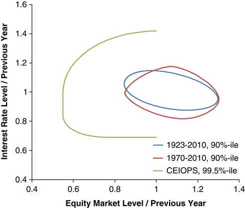
The last section of the paper investigates combined stress tests and two-way correlations, the latter of which has appeared in recent CEIOPS papers on risk calibration. Finally, there is a discussion of half-spaces as an alternative to the more common quadrant approaches used to consider extreme events.

3.1 Economic Capital

3.1.1 A financial institution, be it an insurance company or a bank, faces a multitude of risks that could cause a financial loss. Economic capital is the realistic amount of capital that is needed to cover losses at a certain risk tolerance level. It captures a wide spectrum of risks such as insurance risk, market risk, credit risk and operational risk, as well as dependencies between them and various other complexities like transferability of capital, and expresses all of this as a single number.

3.1.2 There are three main components of an economic capital definition:

1. (i) risk measure

2. (ii) probability threshold and

3. (iii) time horizon

A company may do an economic capital calculations according to an external criteria laid down by the regulators for regulatory capital purposes or other criteria e.g. to satisfy specific standards prescribed by a rating agency.

3.1.3 Currently, the most popular risk measure that is used in banking and insurance is the one-year 99.5% Value at Risk (VaR). For example, under the UK's Individual Capital Assessment (ICA) regime and Solvency II, an insurance company needs to hold enough capital such that there is a probability of 99.5% of survival over a one-year time horizon, or in other words the probability of insolvency over 12-months is no more than 0.5%.

3.1.4 However, not all risks the company is facing will cause losses at the same time. Some areas of business may experience extremely high financial losses whilst others average losses, or even profits – an effect known as ‘diversification’. Many firms calculate the capital requirement for each risk in isolation, ignoring the effect of other risks. The effect of diversification is visible when the overall capital required for an insurance company at the 99.5% level is less than the sum of the 99.5% individual capital amounts for each risk.

3.1.5 The extent to which the aggregate 99.5% capital differs from a straight sum of the 99.5% individual capital amounts is a measure of the level of diversification between risks. The lower the degree of dependency between risks the greater the diversification benefit.

3.1.6 Diversification is not the only balancing item to reconcile single risk capital calculations to a total company level. Interaction effects may also play a part, where a development in one risk may amplify another. For example, an insured loss may be recoverable after some delay from reinsurance cover, creating an exposure to the risk of reinsurer default in the meantime.

3.1.7 The diversification benefit depends, among other things, on the level from which aggregation starts. For example, if we started aggregating at the “equities, property, fixed interest” level we are going to get a different diversification benefit than if we start aggregating at the UK equities, US equities, Asian equities, UK fixed interest, US fixed interest, Asian fixed interest level.

3.1.8 The extent of the level of diversification between risks varies from company to company. In fact, the recent CRO Forum QIS 4 benchmarking study of 2008 suggested that diversification reduces economic capital by around 40% on average.

3.2 Regulatory Developments

The use of economic capital models is far greater today compared with a few years ago. One of the key drivers to their more regular use within financial institutions has been the evolution of legislation for insurance companies and banks. Two of the more influential pieces of legislation have been the developments arising under Basel II (Banking) and Solvency II (Insurance).Footnote 1

3.3 Solvency II – Internal Model Approval

3.3.1 The modelling of dependencies and calculation of the overall diversification benefits goes beyond a pure bottom line insurance company impact. With the advent of the Internal Model Approval Process (‘IMAP’) under Solvency II, and company desires to gain approvalFootnote 3 of their economic capital models for computing the SCR, various other criteria, often otherwise ignored, suddenly become important.

3.3.2 In particular with reference to CEIOPS (2010d).

3.3.2.1 Use Test (Section 3 of the CEIOPS Paper)

1. 1) Senior management, including the administrative or management body shall be able to demonstrate understanding of the internal model and how this fits with their business model and risk-management framework.

2. 2) Senior management, including the administrative or management body shall be able to demonstrate understanding of the limitations of the internal model and that they take account of these limitations in their decision-making.

3. 3) The timely calculation of results is essential. The administrative, management or supervisory body will need to ensure that the undertaking avoids significant time lags between the calculation of model output and the actual use of the model output for decision making purposes.

3.3.2.2 One approach is to require board members to become familiar with say copula methodologies, at least on a very high level, and whatever dependencies are buried inside third party economic scenario generators. An alternative approach is to simplify the models until management can understand how they work.

3.3.2.3 Simplification has some significant advantages, including easier calibration and maintenance as well as a better chance of mistakes being detected as results are open to wider scrutiny. Furthermore with regards to point 3, a simpler model is less likely to suffer from the time lags associated with a more complex model with multiple outputs. Having said that, an overly-simplified model may not be able to cope with such important features of tail dependency and asymmetry. A balance needs to be struck between simplicity and functionality.

3.3.2.4 Statistical Quality Standards (Section 5 of the CEIOPS Paper)

Another important section is that of the Statistical Quality Standards. Here there are many onerous requirements. We have focused on the “Adequate system for measuring diversification effects” and in particular on paragraphs 5.245 and 5.246 of the paper:

4) There should be meaningful support for claiming diversification effects that includes:

1. a) Empirical/Statistical analyses

2. b) Expert judgement of causal relationships

3. c) or a combination of both.

3.3.2.5 Regarding expert judgements, it is important to note that these should be explained and documented in detail and in a well-reasoned manner, including how expert judgement is challenged and reviewed/monitored against actual experience wherever possible.

3.3.2.6 From paragraph 5.246 of the CEIOPS paper:

1. 5) Whatever technique is used for modelling diversification effects, undertakings shall ensure that diversification effects hold not only on average but also in extreme scenarios and scenarios for those quantiles which are used for risk management purposes.

3.3.2.7 Given that correlation coefficients between risks are often set by reference to external studies, e.g. SCR Standard Formula correlations, point 4 above would seem to imply a lot more work needs to be done within insurance organisations to justify their parameter selections. Justification of diversification parameters is likely to prove quite difficult, but it is a necessary and positive development for the insurance industry.

3.3.2.8 External Models and Data (Section 10 of the CEIOPS Paper)

Many insurance companies that use third-party Economic Scenario Generators (ESG) as a part of the economic capital modelling process will need to be able to demonstrate an understanding of the dependency modelling within and the calibration thereof. Furthermore they will need to demonstrate a knowledge of any limitations of such processes.

3.4 Diversifiers and Hedgers and the Importance of Perspective

3.4.1 One of the key roles of insurance risk management is a careful selection of risks to be accepted. Thereafter there are two principle secondary techniques to manage risks:

1. (i) Diversification.

2. (ii) Hedging.

3.4.2 Diversification and hedging, whilst both being used to mitigate risk, rely on different levels of correlation between risks to be their most effective in the minimisation of the overall level of the risk exposure that an organisation faces.

3.4.3 Insurance companies would like to minimise their overall capital needs for a given set of risk exposures and so are interested in the concept of diversification, or in other words, spreading their risks across many different categories. Diversifiers want to avoid high dependence between risks and so are interested in correlations between risks being either small positive numbers, zero or even negative.

3.4.4 In contrast, hedgers are interested in a high level of positive correlation between the gross underlying risk exposure and the relevant insurance/capital market instrument used to mitigate such risk.

3.4.5 A simple example of an insurance risk management instrument would be to use reinsurance to reduce the gross insurance loss exposure. The risk mitigating impacts of the two principle types of reinsurance, namely quote share and excess of loss, are a function of the overall level of gross exposure and the detailed specifics of the reinsurance contracts in question. The relationship (or ‘correlation’) between the gross and net losses will thus be a function of the overall level of gross insurance losses.

3.4.6 Another example from capital markets is where available derivatives from banks might be on a standard index portfolio, and available only for terms shorter than the underlying insurance policy. To hedge, the insurer buys the guarantees that are available, hoping for a sufficiently high correlation between risks.

4.1 Dependency Structures

4.1.1 It is helpful to make a distinction between the economic drivers of risks facing an insurer and the monetary balance sheet effect. The economic drivers might include interest rates, mortality, natural catastrophes and credit indices, most of which can be observed external to the insurer. The monetary effect is a function of these drivers, sometimes a very complicated one, and is specific to the insurer.

4.1.2 Within a single period value-at-risk model, the drivers are described by a multivariate joint probability distribution. Given that multivariate distribution, we can calculate the marginal distribution of each risk, that is, the distribution of each risk in isolation. The marginal distributions constrain but do not determine the joint distribution. The ‘dependency structure’ represents the information contained in the joint distribution but not in the marginal distributions.

4.1.3 There are enough issues alone in estimating the form of the distribution and parameters for the marginal risk distributions before we even consider how they might be linked in a dependency structure. The realistic measurement and modelling of dependencies is one of the most difficult aspects of economic capital modelling facing the insurance and banking industries today.

4.1.4 An unrealistic model of a dependency structure could result in an unrealistic optimistic or pessimistic view of an enterprise, despite the fact that the individual capital components themselves may be quite reasonable.

4.2 What Do We Mean by Dependency

4.2.1 In everyday language a lot of us use the words ‘correlation’ and ‘dependency’ interchangeably. Quite often a correlation coefficient is used in situations when we need to measure the strength of dependency between two random variables. In fact, it is very important to remember that correlation is just a special case of dependency. It quantifies a linear relationship between two random variables whilst dependency deals with any kind of relationship.

4.2.2 Dependency between two random variables (e.g. risk factors) means that there is some link between them, i.e. information about one random variable tells you something about the value of the other random variable. One extreme is perfect dependence; if you know the value of one random variable, you know exactly what the value of the other random variable is. The other extreme is independence; the value of one random variable does not enable you to make any predictions about the value of the other random variable.

4.2.3 Dependence between two random variables can be strong but such a relationship does not need to follow a linear pattern. Consider the simple example in Figure 1 of two random variables, X and Y. Let us suppose that U is uniformly distributed on [0,1] and, for α = 0.4:

Then Y = 1/X so these distributions are dependent.

Figure 1 Dependent Variables with Low Correlation.

Although Y = 1/X, a decreasing function of X, the correlation between X and Y is not −100% but only −29%. This is because the relationship between X and Y is non-linear. Taking different values of α, we can generate examples with correlations between −100% (for α close to zero), rising to zero as α approaches 0.5.

This is easy to investigate by simulation, or by the analytical formula for the correlation:

4.2.4 One of the reasons for the popularity of correlation in finance is that it is used in variance-covariance matrices as part of Modern Portfolio Theory, which is based on the normal (or more correctly, elliptical) distribution. However, in reality, a lot of financial risks that are dealt with in economic capital modelling and other actuarial work are not adequately described by the normal distribution, see Shaw (Reference Shaw2007), or indeed by an elliptical distribution. Many of these risks exhibit asymmetry and ‘fatter’ tails than described by the normal distribution, especially in non-life insurance, and so relying solely on correlation as a measure of dependency between risks can be very misleading. Moreover, by definition, correlation is a constant scalar coefficient.

4.2.5 Market experience over the last year has led many firms to re-estimate the parameters underlying their models. In some cases, particularly for credit markets this has led to dramatic parameter revisions. This applies both to marginal distributions and to dependency structures. One possible interpretation, asserted by CEIOPS in CEIOPS (2010c) is that the linear correlations between various assets classes turned out to be significantly higher than have been observed historically. Embrechts et al. (Reference Embrechts, McNeil and Straumann1999) provide the following good summary of the deficiencies of using correlation solely as a measure of dependency:

D1. Correlation is simply a scalar measure of dependency. It cannot tell us everything we would like to know about the dependency structure of risks.

D2. Possible values of correlation depend on the marginal distribution of the risks. All values between −1 and 1 are not necessarily attainable. This means, a model might be impossible to calibrate to certain correlation values.

D3. Perfectly positively dependent risks do not necessarily have a correlation of 1. Perfectly negatively dependent risks do not necessarily have a correlation of −1.

D4. A correlation of zero does not imply independence between risks.

D5. Correlation is not invariant under monotonic transformations. For example, log(X) and log(Y) generally do not have the same correlation as X and Y.

D6. Correlation is only defined when the variances of the risks are finite. It is not an appropriate dependency measure for very heavy-tailed risks where variances appear infinite.

4.2.6 Sections 4.3 to 4.5 describe the different types of correlation.

4.3 Pearson Correlation Coefficient

We begin with by considering a pair of random variables X, Y with finite variances.

4.3.1 Two Variables

4.3.1.1 The Pearson correlation coefficient between X and Y is:

4.3.1.2 If we have a sample of n observations x_i and y_i where i = 1, 2, …, n, then the sample correlation coefficient, also know as Pearson product-moment correlation coefficient can be used to estimate the correlation between X and Y:

4.3.1.3 Pearson correlation has the following important properties:

• – The correlation is 1 in the case of an increasing linear relationship, −1 in the case of a decreasing linear relationship, and some value in between in all other cases.

• – The closer the coefficient is to either −1 or 1, the stronger the correlation between the variables. ||ρ_L[X,Y]|| = 1 if and only if there exist a, b ≠ 0 such that Y = a + bX.

• – If the variables are independent then the correlation is 0, but the converse is not true because the correlation coefficient detects only linear dependencies between two variables. For example, suppose the random variable X is uniformly distributed on the interval from −1 to 1, and Y = X². Then Y is completely determined by X, so that X and Y are dependent, but their correlation is zero; they are uncorrelated.

• – However, in the special case when X and Y are jointly normally distributed, zero correlation is equivalent to independence.

• – Linear correlation is invariant under a linear transformation: ρ_L[a ₁ + b ₁X, a ₂ + b ₂Y] = sign(b ₁b ₂) × ρ_L[X,Y] for all real a₁, a₂ and b ₁, b ₂ ≠ 0

• – Linear correlation is not invariant under an arbitrary non-linear monotonic transformation T: ρ_L[T(X),T(Y)] ≠ ρ_L[X,Y].

4.3.1.4 There are many practical reasons for using of the Pearson correlation coefficient:

• – The Pearson correlation is easy to calculate.

• – The Pearson correlation is covered in many elementary statistical courses, so is likely to be familiar to a broader range of professionals making communication easier.

• – Given standard deviations and correlations of a vector of variables, it is simple to calculate standard deviations for sums and differences of those vector elements, as well as correlations between different linear combinations.

• – In the context of elliptically contoured distributions, the correlation matrix uniquely determines the dependence structure.

• – Where many risks are correlated, the correlations form a correlation matrix. The necessary and sufficient conditions for a correlation matrix to be feasible are well understood, and rapid tests exist even for high dimensional distributions.

4.3.2 Correlation Matrix

4.3.2.1 Consider vectors of random variables X = (X ₁,…,X_n)^t and Y = (Y ₁,…,Y_n)^t. Then, given pairwise covariances Cov[X,Y] and correlations ρ(X,Y) for an n × n correlation matrix we define:

Such nxn matrices have to be symmetric and Positive Semi-Definite (‘PSD’). (See Appendix A for a definition of PSD).

4.3.2.2 Rank correlation is an alternative to the use of linear correlation as a measure of dependency. The two most common types of rank correlation are:

1. (i) Spearman coefficient; and

2. (ii) Kendall Tau correlation.

Both of them are commonly used.

4.4 Spearman Coefficient

4.5 Kendall Tau Correlation

4.5.1 The Kendall Tau correlation measures dependency as the tendency of two variables, X and Y, to move in the same (opposite) direction. Let (X_i,Y_i) and (X_j,Y_j) be a pair of observations of X and Y.

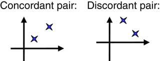
4.5.2 If (X_j−X_i) and (Y_j−Y_i) have the same sign, then we say that the pair is concordant, if they have opposite signs, then we say that the pair is discordant. Figure 2 illustrates concordant and discordant pairs in the (x, y)-plane.

Figure 2 Example of Concordant and Discordant pairs.

4.6 Numerical Example

4.6.1 Let us consider Table 1 with 10 joint observations from two risk factors, A and B:

Table 1 Example of calculations for risk factors A and B.

4.6.2 The Linear correlation coefficient is equal to 0.21 whereas the Spearman correlation is equal to −0.19. This latter calculation involving the correlation of the ranks between the two risks. We note that the Spearman correlation is very different from the linear correlation. This is because the linear correlation is heavily affected by one outlier (the last observation).

4.6.3 Kendall's Tau is equal to −0.16 and is calculated as (19–26)/45. It is close to the Spearman correlation, as they are both rank correlations and not affected by the outlier.

5.1 Risk Aggregation Framework

5.1.1 A prima facie reason for the consideration of different dependency modelling structures is risk aggregation in computing overall economic capital levels for insurance companies and banks.

5.1.2 A common approach for deriving economic capital is by first assessing the individual risk components and then considering possible techniques to aggregate these components to derive an overall capital number. This approach is a feature of the first four methods that we discuss in sections 5.3 to 5.6.

5.1.3 One of the natural ways to model a joint behaviour of multiple risks is to come up with their multivariate distribution function. This leads to the use of copulas (see sections 5.6 and 8) which provide a way of combining stand-alone marginal risk distributions into a multivariate distribution.

5.2 Risk Aggregation Methodologies

Insurance companies and banks differ in their approaches to economic capital risk aggregation, some techniques being more sophisticated than others. The most common broad categories of methods used in financial modelling are:

• – Simple Summation (no allowance for diversification benefits).

• – Fixed Diversification percentage.

• – Variance-covariance matrix (quite often called the ‘Correlation Matrix’ or ‘Sum of Squares’ approach).

• – Copulas.

• – Causal Modelling (an abstract model that uses cause and effect logic to describe the behavior of an insurance organisation; often referred to as an ‘integrated model’ using CEIOPS Solvency II nomenclature). This method is often used in combination with the above methods, such as variance-covariance matrix or copulas.

5.3 Simple Summation

This involves adding together the stand alone marginal risk capital amounts. It ignores potential diversification benefits and produces an upper bound for the economic capital number. Mathematically this is equivalent to assuming a perfect dependency between risks, e.g. 100% correlation.

5.4 Fixed Diversification Percentage

This method is very similar to the straight summation as described in 5.3 above, however it assumes a fixed percentage deduction from the overall capital figure.

5.5 Variance-Covariance Matrix

5.5.1 The correlation matrix approach is where capital is first calculated on a stand alone basis for each risk and then aggregated using a correlation matrix. In this calculation there is no prerequisite for the stand alone marginal risk distribution to be known, however such stand alone capital for many risks is often calculated from prior determined marginal risk in the economic capital modelling process.

5.5.2 The correlations may be estimated using conventional techniques. An alternative is to back-solve parameters to reproduce the answers to specified aggregation tests. The resulting parameters are sometimes called tail correlations or quadrant correlations.

5.6 Copulas

5.6.1 The copula approach is different, in that it involves a Monte Carlo simulation with the full marginal risk distribution of each risk and a copula function to produce a meaningful aggregate risk distribution. The simplest copulas from the calibration point of view are the Gaussian and t copula, more of which will be said later.

5.6.2 This section gives a brief intuitive introduction to the concept of copulas, whereas section 8 goes into more technical details on this topic.

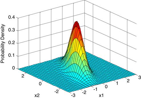
5.6.3 Let us consider two random variables X and Y. A range of outcomes for each variable on a stand alone basis can be represented by a marginal risk distribution function, given by its two-dimensional Probability Density Function (‘PDF’) or Cumulative Density Function (‘CDF’).

5.6.4 In addition, we might happen to know the distribution law which describes the joint distribution of any pair of values (X,Y), i.e. the three-dimensional surface. Visually one can think of loss amounts on the x-axis and y-axis for X and Y respectively with the z-axis representing the value of either the joint PDF or CDF. If the joint distribution is known, it gives us the best possible information about the behaviour of both variables in aggregate. However, in practice, if we have a large number of risk variables, such as equity, fixed interest, property, non-life underwriting risk, non-life reserving risk etc. it is very difficult to specify a multivariate joint distribution between all risks.

5.6.5 A way of dealing with this difficulty is to split the problem into two parts as illustrated by Figure 3:

Figure 3 Simple representation of a Copula.

• – The first part describes the individual behaviour of each risk in isolation, i.e. the stand alone marginal risk distribution (‘MRD’) and

• – The second part (which in itself is a distribution function) the dependency structure between the risk variables. This second part is known as a copula of the distribution:

5.7 Causal Modelling

5.7.1 Causal modelling is best explained as common risk drivers which impact risks often in a non-linear fashion. This is the usual method for capturing dependencies within economic scenario generators. A typical example would be inflation being derived from simulated nominal and real yield curves, which in turn is linked to the simulation of insurance losses. This method is often used in combination with others, for example even in causal modelling it is not possible to formulate all potential risk relationships credibly and so techniques such as correlation matrices or copulas are often used to deal with the residual dependency risk relationships.

5.7.3 Causal Loop Diagram for the Growth or Decline of UK Life Insurance Companies

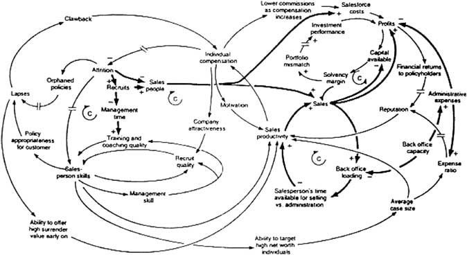
5.7.3.1 These models can get quite complex, as is illustrated by the causal loop diagram in Figure 4 to explain the growth or decline of UK life insurance organisations.

Figure 4 Casual Loop Diagram for Growth or Decline of UK insurance companies.

Source: Robert A Taylor (2008).“Feedback”. U.S. Department of Energy's Introduction to System Dynamics (2008).

5.7.3.2 There are various features from Figure 4 worth mentioning:

• – The model's negative feedback loops are identified by ‘Cs’ which stand for ‘Counteracting loops’.

• – The symbols ‘//’ are used to indicate places where there is a significant delay between cause and effect.

• – The thicker lines are used to identify the feedback loops and links that the reader should focus on.

5.7.3.3 It is clear that a decision maker would not find it easy to think through the model dynamics based on such diagrams alone. As with the copula approach to economic capital calculation, the causal modeling approach would involve Monte Carlo simulation.

5.8 Natural Catastrophe vs. Reinsurance Credit Risk Aggregation

5.8.1 Companies often use a combination of different methods that we have described so far. For example, each insurance company within an insurance group may have models that operate in sufficient detail for its own purposes, but all companies within the group use common economic model output and disaster scenarios that imply dependency when risk is viewed at a group level.

5.8.2 The modelling of reinsurance credit risk, i.e. the loss associated with the failure of reinsurance counterparties is a good example of the different levels of modelling granularity.

5.8.3 One of the key dependencies for non-life insurance companies is between Catastrophe underwriting risk (‘Cat UW risk’) and Reinsurance credit risk (‘RI credit risk’). If a low frequency, high severity natural catastrophe loss event were to occur, then a non-life company writing property related business may see a large increase in reinsurance credit risk, due to both an increased likelihood of default by its reinsurers and an increased exposure i.e. larger reinsurance recoveries.

5.8.4 Different methods are possible to reflect this dependency structure between Cat UW Risk and Reinsurance credit risk. These are described as follows:

1. 1) The simplest of the approaches would involve Catastrophe Underwriting risk (“Cat UW risk”) and Reinsurance credit risk (‘RI credit risk’) as separate entries within a variance-covariance matrix.

   • – The marginal risk capital calculation for RI credit risk would be based on the expected level of reinsurance recoveries and other risk factors. The exposure would include the run-off of the opening balance sheet values and the expected incremental exposure from one year's new business.

   • – The selected correlation coefficient for use within the correlation matrix would reflect:

     • (i) dependency relationships between the levels of exposure i.e. gross insurance losses (‘Cat UW risk’) and reinsurance recoveries via the reinsurance arrangements; and

     • (ii) more complex relationships involving reinsurance default rates and loss given default being functions of the level of gross insurance loss events.

2. 2) An alternative slightly more complex approach would involve the Cat UW risk marginal risk distribution also capturing the associated RI Credit risk associated with Cat UW risk. The Cat UW risk capital now being larger than the value of CAT UW risk calculated in 1.

   • – Given that it is common for Cat UW risk modelling to involve the simulation of gross losses and reinsurance recoveries, such methods would enable the modeller to capture the varying reinsurance loss exposure more accurately via the direct structural relationship between the exposures.

   • – In this eventuality the RI Credit risk marginal capital calculation would only be in respect of reinsurance recoveries associated with the prior year's business.

   • – Despite there now being a direct causal link between the simulated gross insurance losses and the reinsurance recoveries for new business, there is still left the potential residual risk dependency relationship between a large natural catastrophe and the indirect impact on reinsurance credit risk variables like default probabilities. This residual dependency risk could be handled either though a selected correlation within a variance-covariance matrix calculation or by copula simulation.

3. 3) More complex causal modelling methods could involve:

   • –

     • (i) Reinsurance Default Probabilities (PD) and Loss Given Default (LGD) being a function of insurance losses and/or asset values and /or:

     • (ii) stochastic interest rates in the discounting of the reinsurance loss payments in the RI Credit risk calculation given that economic capital calculations are on a present value basis.

5.8.5 The last method, whilst being more intuitive, than the earlier methods, does at the same time introduce more uncertainly in terms of both model risk and parameter risk.

6.1 Spurious Relationships

6.1.1 It is important when looking at empirical results that spurious relationships are not mistaken for dependency relationships between risks.

6.1.2 In statistics a spurious relationshipFootnote 4 is a mathematical relationship in which two occurrences have no causal connection, yet it may be inferred that there is one. “Correlation does not imply causation” is often used to point out that correlation does not imply that one variable causes the other. However, the presence of a non-zero correlation may hint that a relationship does exist.

6.1.3 Edward Tufte (Reference Tufte2006) puts it succinctly:

6.1.6 Spurious Regression Example

6.1.6.1 Consider 2 random walk time series, X_t and Y_t as follows:

where:

ε_t and δ_t are N(0,1) distributed

X₀ = Y₀ = 5.

6.1.6.2 Given this, a random sample of 100 values for each of X and Y for t = 0 to 99 has been generated. Using this output the linear correlation and R² have been calculated.

6.1.6.3 X and Y are not related and yet it is common, to observe high correlations.

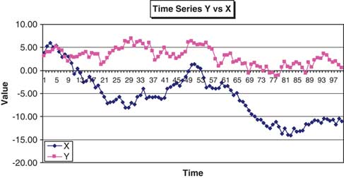
6.1.3.4 Figures 5, 6 and 7 show:

Figure 5 Linear Regression of Y vs X.

Figure 6 Time Series of Y vs X.

Figure 7 Residuals from the linear regression.

1. (i) Linear regression between X and Y. (Figure 5)

2. (ii) Time Series of X and Y (Figure 6)

3. (iii) Residuals from the linear regression (Figure 7).

6.1.3.5 In this random example, the observed correlation between X and Y is 56.5% and 5.9% between the residuals (any difference from zero due to simulation error). The time series plots in Figure 6 for X and Y look plausible for typical financial variables and yet we conclude they have a large positive correlation when in fact there no relationship between them at all. Moreover, there is significant autocorrelation in the residuals leading one to reject the linear regression model as a measure of the relationship. In fact, this is illustrative of the fact that trending variables, which are often a feature of economic and financial time series data, are likely to lead to a regression with high values of R², regardless of whether they are related or not. Differencing variables (changes) eliminates trends and thus avoids spurious regression, so it is important to consider the nature of the variables being used to determine the correlation of interest.

6.2 Correlation and Linearity (Anscombe's Quartet)

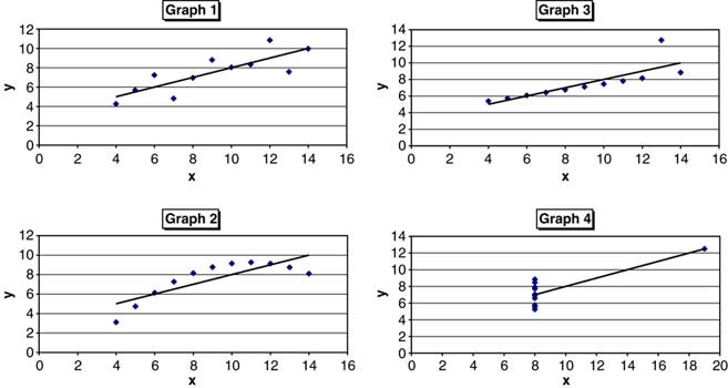
The Pearson correlation coefficient indicates the strength of a linear relationship between two risks, but it alone is often not sufficient to evaluate the strength of this relationship. This is illustrated with a study of sets of scatter plots of what is known as Anscombe's quartet, created by Francis Anscombe (Reference Anscombe1973). The y variables have the same mean, standard deviation, linear correlation and regression line and yet in all four cases the distribution of the variables is markedly different.

6.2.1 Anscombe's Quartet

Anscombe's quartet consists of four data sets which have the same identical statistical properties but which are very different to each other when viewed graphically. The different graphs are labelled 1 through to 4. The linear regression line for each set of points is given by y = 3 + 0.5x. The statistics for all four data sets are shown in Table 2.

Table 2 Anscombe's Quartet Statistics.

6.2.2 Comments on Figure 8

Graph 1 – What one would expect when considering two correlated variables that follow the assumption of normality.

Graph 2 – The relationship is not linear but an obvious non-linear relationship exists.

Graph 3 – The linear relationship is perfect except for one outlier.

Graph 4 – The relationship between variables is not linear but one outlier is enough to give a correlation of 0.81 and make it appear as though there is one.

The numerical examples in Figure 8 demonstrate that the correlation coefficient, as a statistic cannot replace a more detailed examination of the data patterns that may exist.

Figure 8 The four different graphs of Anscombe's Quartet.

6.3 Biases introduced by the way we look at Data

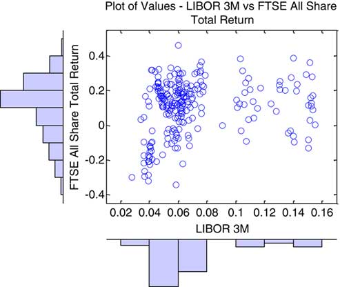
6.3.1 Following on from section 6.2, we address the potential issues arising from the different ways that we may investigate the same data set. Ideally data visualisation needs to take place in more than one framework. For example, a typical visualisation of the dependency structure between two risks is through the use of a scatter plot, as in Figure 9. Here the Pearson correlation coefficient between the two risks X and Y is 55.1%.

Figure 9 Linear Regression of Y vs. X.

6.3.2 However, if we plot risks X and Y as time series (Figure 10) we see quite a marked pattern in the differences in their relationship over time. The dependency between the two risks is time-varying, the nature of which will not be picked up in graphical representations such as a scatter plot. The scatter plot in essence disregarding any historical trends that may be present in the data.

Figure 10 Time Series of Y vs X.

6.3.3 This is not to say that a scatter plot is not useful but that it should perhaps not be the only visual aid used in the computation of correlation parameters.

6.4 Wrong-Way Risk

6.4.1 Sections 6.4 to 6.7 look at miscellaneous topics that each in their own right and illustrate some of the potential issues arising when parameterisation and modelling dependency structures within economic capital models. We begin with a discussion of the so-called ‘wrong-way risk’.

6.4.2 The way that risks are aggregated relates to the scope of inter-risk diversification, i.e. to the idea that an aggregation of risks will not be larger that the sum of its components.

6.4.3 With risks aggregation across different portfolios or business units, some of the assumptions may fail to hold. One possible reason for the aggregate to require more capital than the sum of the capital for each component is the nature of the risk measure. For example, the VaR measure can be shown to fail the subadditivity property of a coherent risk measure. It is possible to construct examples where the VaR of a combination of risks is greater than the sum of the VaR of the individual constituent parts.

6.4.4 Another reason is more complex and subtle, the so-called ‘wrong-way risk’. This is also sometimes called ‘interaction’ or ‘nonlinearity’.

6.4.5 With the ‘wrong-way risk’ the reason why the aggregate risk may be greater than the sum of the parts is not related to the choice of risk metric, but because one risk may amplify the effect of another. Measurement of risks one at a time may not detect this amplification. This issue is more prevalent with the variance-covariance matrix approach to risk aggregation than the other approaches we have identified.

6.4.6 For example, measuring separately the market and credit risk components in a portfolio of foreign currency denominated loans with a currency hedge can underestimate risk as a default may result in an over-hedge of subsequent currency movements.

6.4.7 Another example is a follow on from section 5.8 and the discussion of different types of modelling of Natural Catastrophe and Reinsurance Credit Risk. The two risks types are often modelled separately before being combined. A situation where a catastrophe increases reinsurance due as probability of default is the ‘wrong-way risk’. The standard formula makes an assumption that loss in any scenario can be expressed as a simple sum of risks from different sources, but in this example there is an arbitrariness in assessing whether a reinsurance bad debt on a larger than expected recovery is classified as default risk or natural catastrophe risk. The answer is that it depends on the order in which the risks are analysed – an effect familiar to actuaries through analysis of change. As the result is no longer a sum of marginal risks, the correlation formula based on the variance of a sum, no longer applies.

6.4.8 Modelling tail dependency in underlying risk drivers is no remedy for wrong-way risk. Instead, it is necessary to model carefully the way in which a firms net assets depends on risk drivers, including a consideration of effects when more than risk materialises at once. One method of capturing this is to use the combined scenario approach outlined in Solvency II, whose mathematical basis is covered in McNeil & Smith (Reference Mcneil and Smith2009).

6.5 Multivariate Distributions: The Curse of Dimensionality

6.5.1 There are times when one may want to calibrate dependency relationships by looking simultaneously at all risks together, rather than the more common approach of two risks at a time, whether estimating correlation coefficients between a pair of risks, or determining parameters for specific copulas. For example, if there are three risks: A,B,C of interest, this would involve looking at the joint distribution of all three (A,B,C), rather than the separate analysis of the three pair combinations (A,B), (A,C) and (B,C).

6.5.2 However, the estimation of multivariate distributions suffers from the so-called ‘curse of dimensionality’.

6.5.3 Here is an example of the problem. An insurer itemises the risks to which it is exposed, resulting in a short list of 200 risks. Let us suppose that 90 years of clean and relevant historical data is available with annual observations, for each risk. For some risks, far fewer than 90 years relevant data is available. Having 100 years data provides more statistical input that is usually available. With such a data set, we may be able to estimate not only location and dispersion but perhaps also some measures of asymmetry and tail fatness.

6.5.4 However, in the multivariate case, the number of parameters proliferates relative to the number of observations. For example, suppose we are to estimate a correlation matrix. A 200 × 200 correlation matrix contains 19,900 distinct elements. Out of 40,000 elements, the 200 diagonal elements are all 1, and as the matrix is symmetric the remaining 19,900 elements each appear twice, once below and once above the diagonal.

6.5.5 The number of data points is only 18,000, this being 200 risks multiplied by 90 annual observations. No continuous calibration methodology can map the possible data sets onto the set of possible correlation matrices. There will always be some correlation matrices that are mathematically valid but inaccessible, that is, which cannot arise for any input data set. The more limited the data, the greater the extent of inaccessible matrices.

6.5.6 It may be argued that it is desirable to capture aspects of distribution beyond mean and variance. For example, it may be desirable to capture skewness and tail fatness. It may be desirable to capture aspects of dependency beyond correlations, such as quadrant correlations or tail dependency. All of these introduce additional parameters, inevitably increasing the extent of inaccessible correlation matrices.

6.6 Multivariate Distributions: Multivariate Model Selection

Given the wide range of possible multivariate models, and the impossibility of distinguishing between them on data alone, other supplementary criteria come into play.

These might include:

• – Computational ease of calibration, validation or simulation

• – Results-driven model selection

• – Consensus – using a similar approach to other firms

• – Mathematically ‘natural’ models.

We examine each of these criteria in turn.

6.7 Ten Properties of Good Calibration

6.7.1 A realistic economic capital model should ideally have robust calibration. There remains the question therefore of what constitutes a ‘good calibration’. A natural statistical approach is to select a family of distributions and to estimate these using a combination of historic data and expert guesswork. Several generic approaches exist for distribution estimation, including the method of maximum likelihood, as well as methods based on setting fitted statistics such as means, correlations, rank correlations or kurtosis to their empirically estimated counterparts.

6.7.2 There are good and bad ways to go about calibrations. Choices to adopt a particular approach usually involve some sort of trade-off between different criteria. Some attributes of a good calibration process are as follows:

• – Statistical power – This means that estimated parameters are likely to be close to the true parameters.

• – Robust Process – The estimation process converges to a unique solution (does not get stuck in an endless loop nor iterate between solutions), estimated models can be computed quickly and the fitted model varies continuously as a function of the data and responds logically to new data

• – Symmetries – The estimation process is preserved under various transformations of the data, e.g. if we rotate the historic risk vectors then fitted distribution is the corresponding rotation of the unrotated fit.

• – Parsimony – The number of parameters used is minimised in order to produce the simplest possible model. Parameters are included only if justified by the data.

• – Surjection – Any underlying distribution is capable of arising as a fit given sufficient data; the calibration process does not exclude significant model types.

• – Parallel threading – Individual parameters each follow a transparent process from data to parameter value, which can be verified manually, communicated graphically, explained to non-experts and consequences understood. The alternative is an estimation process where all parameters emerge simultaneously from a single complicated calculation.

• – Consistency – Input conflicts can easily be avoided or at least remedied. An example of input conflicts is a correlation matrix that is not positive definite; each individual assumption is valid but together they are not.

• – Inclusion – Different methodologies can be combined for different parameters. For example some parameters may be estimated from historic data, others taken from published analysis, others from expert views and yet others from peer group surveys.

• – Evolution – Existing software can be re-used, or cheap software licensed. The need for technical re-training, bespoke development or explaining unfamiliar concepts to regulators, is minimised.

• – Surplus suitability – The construction of any model of surplus (in short available capital) should lend itself to fast and accurate calculations of key percentiles of the surplus function, as well as to supplementary calculations such as marginal attribution of capital requirements.

7.1 Methodology

7.1.1 Introduction

7.1.1.1 This method allows for a full pattern of risk interactions with the assumption of differing pairwise correlations between risks. The overall level of diversification between risks is dependent on the levels of these correlations.

7.1.1.2 The capital for an insurance company with n risks is calculated by use of the following variance-covariance matrix formula:

Where:

• – C_i is the stand alone capital amount for the i^th risk

• – Correlation coefficient ρ_ij for risks i and j allows for the diversification between risks.

7.1.1.3 When correlations are all equal to 1, the calculation is equivalent to the sum of stand-alone capital amounts. If the risks are all independent i.e. the correlation coefficients between risks i and j are all equal to zero then the total capital is equal to:

7.2 Advantages and Disadvantages of Variance-covariance Matrix Approach

Advantages:

• – Relatively simple, intuitive and transparent.

• – Facilitates a consensus of typical correlations for use by companies.

• – The use of a cascade of correlation matrices permits the easy addition of further risks, from a new business unit, subsidiary or risk category.

• – Correlation is the only form of dependency that a lot of non-specialists are familiar with. This makes communication easier than some of the more sophisticated methods described in sections 8 and 10.

Disadvantages:

• – Risks where we have empirical evidence of correlations (mainly reliable market data) are very few and so there is a heavy reliance on a subjective ‘expert opinion’ to determine correlations.

• – The variance-covariance matrix approach implies that the underlying risks are normally (or elliptically) distributed.

• – Underestimates the effects of skewed distributions and does not allow for potential heavier dependency in the tail.

• – The value of correlations is sensitive to the underlying marginal risk distributions.

• – A correlation matrix has to satisfy certain conditions (e.g. is Positive Semi-Definite). These are often ignored in practice.

• – All cause-effect structures cannot be properly modelled.

• – Does not capture non-linearities.

7.3 Risk Granularity

7.3.1 The finer the level of risk classification (i.e. a more granular subdivision of risk) within a variance-covariance matrix, the lower the intra-risk diversification (i.e. diversification within a risk category) and the greater the inter-risk diversification (i.e. the diversification between risk categories). Differences in approaches will generally lead to differences in the economic capital number given the complexity of re-working all of the various risk dependency relationships.

7.3.2 Sometimes the economic capital calculation will feature a series of ‘nested’ variance-covariance matrices. An example of this is the method adopted within the standard formula approach to the Solvency II Solvency Capital requirement (‘SCR’) for QIS 4 and as described in CEIOPS (2008).

7.3.3 Table 3 details the correlation matrix that is used to aggregate the individual capital amounts for each of the five main risk categories to derive the Basic SCR. Market Risk capital (SCR Market) is one of the major risk capital categories within this process.

Table 3 QIS 4 SCR Correlation Matrix.

7.3.4 Table 4 shows the nested Market Risk correlation matrix, i.e. the matrix that is used to aggregate the individual capital amounts in respect of different types of market risk e.g. interest rates, equities etc to derive an overall Market Risk capital number for use in Table 3.

Table 4 QIS 4 Market Risk Correlation Matrix.

7.3.5 It is a common practice for many life insurance companies to aggregate individual stress tests results by using the variance-covariance matrix approach. Some non-life insurance companiesFootnote 5 use this approach as well. However, more and more companies (at the moment mostly in the non-life area, although with life offices also gradually moving in the same direction), use more sophisticated mathematical models involving copulas and causal modelling.

7.4 Simpler Variants

7.5 Parameterisation

7.5.1 Parameterisation of the variables used to model dependency structures in economic capital models is very often difficult. Many issues arise, not only in the estimation of parameters themselves, e.g. correlations for use in a variance-covariance matrix calculation, but also how these parameters evolve over time as a result of changes in economic indicators, business cycles or underwriting cycles.

7.5.2 Some of the typical questions arising are:

• – Estimation of correlation coefficients for use in a variance-covariance matrix.

• – What sources of data and information are needed for the parameterisation exercise?

• – What sources of data and information is currently available?

• – How accurate, reliable and credible are the sources of data and information available?

7.5.3 The following is a list of possible approaches:

• – Empirical estimation using historical time series data.

• – Use of expert judgement or industry benchmarks.

• – Ranking method, e.g. using Low, Medium and High rankings.

7.5.4 Paragraphs 7.5.5 to 7.5.7 deal with each of these in turn.

7.5.7 Low, Medium and High Rankings

7.5.7.1 In the absence of any data analysis organisations may fall back on the use of Zero, Low, Medium or High correlation rankings or similar grading based on a subjective assessment of the main risk pairings. The correlation coefficients allocated to these groupings are determined in advance based on prior studies. But what do we actually mean by Medium correlation, which could be regarded as rather arbitrary. It could mean 30%, 40%, 50% or somewhere in between. In addition, the actual values within each category are often dependent on the nature of their use.

7.5.7.2 The following in Table 5 illustrates the range of realistic correlations that may appear in each of the correlation groupings, but others could equally be valid.

Table 5 Correlation Ranking Ranges.

7.5.7.3 Categorising dependencies as either Low, Medium or High is sometimes underplayed by commentators as an approach that should be limited to situations when there is no more accurate approach as though correlation measurement was a mere formality.

7.5.9 Estimating Correlations with Variation in the Length of Time Series Data

7.5.9.1 Figures 11 and 12 show annual time series data for 1988 to 2008 for the following:

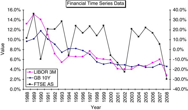
Figure 11 Time Series for LIBOR 3M vs GB 10 Y vs FTSE AS.

Figure 12 Time Series for GB 10 Y vs CS AAA vs CS BBB.

• – LIBOR 3M rateFootnote 6.

• – UK 10 year Government Bond yield (GB 10Y).

• – FTSE All Share Total Return 12-months ending 31/12/YY (‘FTSE AS’).

• – Credit Spread for AAA rated 10 year bonds as at 31/12/YY (‘CS AAA’).

• – Credit Spread for BBB rated 10 year bonds as at 31/12/YY (‘CS BBB’).

7.5.9.2 Figure 11 shows a line graph of the values for the first three indices, whilst Figure 12 shows a similar graph for GB 10Y vs CS AAA vs CS BBB.

7.5.9.3 On inspection of Figure 11 it is clear that the FTSE AS annual return shows a cycle with peaks and troughs over the period 1988 to 2008. Both LIBOR 3M and GB 10Y exhibit downward trends over the same period and furthermore the LIBOR 3M and GB 10Y graphs crossover at a number of different points, indicating the changing shapes in the yield curve, either upward sloping, downward sloping or inverted yield curves.

7.5.9.4 For Figure 12 however, the general decrease in GB 10Y contrasts with the relatively flat credit spreads until 2006 onwards when there has been a sharp rise in the values of both CS AAA and CS BBB reflecting the changing market dynamics following the onset of the recent financial crisis.

7.5.9.5 These relationships between key risk variables changing over time have consequences when one is faced with the estimation of the pairwise correlation coefficients. These comments are not restricted to asset risks in isolation as insurance liability or combined asset/liability time series graphs often show similar patterns.

7.5.9.6 Pairwise correlation coefficients have been estimated between the five different risk types assuming four different time periods, namely:

1. (i) 20 years to 2007;

2. (ii) 15 years to 2007;

3. (iii) 10 years to 2007;

4. (iv) 5 years to 2007.

7.5.9.7 The year 2007 has been chosen rather than 2008 so as to minimise as far as possible the influence of the recent financial crisis on the results comparison. Ideally, monthly data would have been better but for some of the risks the data was only available on an annual basis for time periods longer than 10 years. However, further analysis in the next section on a limited subset of these risks has been performed using monthly data.

7.5.9.8 With only five data points for the five year period 2003 to 2007 the results will be very sensitive to sampling error, as will the results be for the 10 year period and to a lesser extent, periods 15 and 20 years. The results are presented in Table 6.

Table 6 Correlation coefficients for different periods and risks.

7.5.9.9 The four sets of tables clearly show not only the sensitivity of the pairwise correlation coefficients to the time periods chosen for the analysis, but how on some occasions there is a reversal of the correlation signs. These results in conjunction with Figures 11 and 12 illustrate the sensitivity of correlation estimates to the choice of data period and the issues in determining correlation coefficients between risks.

7.5.10 Estimating Correlation Coefficients using Monthly Time Series Data

7.5.10.1 Further analysis has been performed on the following three sets of monthly time series data for the years 1999 to 2008:

• – LIBOR 3M rate as at the end of each month (same notation as before)

• – FTSE 10 Year Gilt Yield as at the end of each month (FTSE G 10Y)

• – FTSE All Share Total Return on a rolling 12-months basis as at the end of each month (same notation as before).

7.5.10.2 Table 7 investigates the correlation between LIBOR 3M and FTSE G 10Y under a number of different calculation bases:

Table 7 Correlation for LIBOR 3M vs FTSE G 10Y.

• – Column ‘12 Mths’ shows the correlation estimate for each year in isolation using 12-months worth of data. For example for year 2005, 81.9% is based on the monthly data from Jan 2005 through to Dec 2005.

• – Column ‘Cum YE 08’ shows the correlation estimated using monthly data assuming a start year (column ‘Year’) through to Dec 2008. For example for year 2005, 74.5% is based on monthly data from Jan 2005 to Dec 2008. This calculation imitating the often used process of estimating correlations from the ‘last x year's worth of data’.

• – Column ‘Cum YE 07’ is a similar calculation to Cum YE 08 but assuming monthly data through to Dec 2007.

7.5.10.3 The latter two calculations are also shown in Figure 13. Observations of note are:

Figure 13 Correlation for LIBOR 3M vs FTSE G 10Y.

• – ‘12 Mths’ correlations are very volatile from year to year.

• – There is more stability in using cumulative monthly data as per Cum YE 08 or Cum YE 07 but even here there is a fair degree of volatility. Both of these calculations appear to indicate a long-term average of around 50%.

7.5.10.4 However, these calculations are looking at correlations between interest rates of different terms. Figure 14 shows similar calculations to Figure 13 but instead for LIBOR 3M vs FTSE AS and this time using 20 years of data. From inspection of this figure it is clear how volatile even these calculations are based on the longer-time series data set.

Figure 14 Correlation for LIBOR 3M vs FTSE AS.

7.6 Variance-Covariance Matrix Cross-Terms

7.6.1 As stated in section 7.1.2, there are many financial institutions, in particular large insurance groups that consist of various subsidiaries, business units (BU) or similar organisational subdivisions. Not only is there a need to calculate economic capital at an individual BU level but also at an overall aggregate level as well.

7.6.2 One of the more common approaches to economic capital modelling, that enables an insurance group to report economic capital at both an (i) aggregate capital level and (ii) BU capital level, is through the use of an enlarged correlation matrix. Data in such a matrix is of the form ‘Organisation/Risk’ e.g. UK /Equity or France/Fixed Interest etc.

7.6.3 In addition, if an insurance company is modelling dependency within an internal model through the use of either a Gaussian or a t copula then it will need the aggregate correlation matrix as described above.

7.6.4 The first stage in the derivation of the overall aggregate correlation matrix is the defining of the correlation matrix at an individual BU level. Once this has been done, there is then the issue of the correlation matrix data entries for the cross-terms such as UK/Equity, France/Fixed Interest etc.

7.6.5 Example

7.6.5.1 Let us consider a simple example of a company with two business units A and B.

Let each BU have two risk factors, 1 and 2 say, where a_xy and b_xy represent the correlation between risks x and y (for all combinations of x, y = 1 and 2) for BU A and BU B respectively.

The correlation matrix for BU A will be ; and the correlation matrix for BU B will be .

Then the enlarged correlation matrix for the whole company would look like:

7.6.5.2 For example, an insurance company might have 15 BUs, each of which has 10 separate risk categories. In this case, the enlarged correlation matrix will be of size 150 × 150.

7.6.5.3 There are several questions immediately raised by this approach:

• – How does one estimate cross terms such as the correlation between a₁ and b₁ etc.

• – Once the cross-terms are filled in, we still need to make sure that the resulting correlation matrix is Positive Semi-Definite (PSD), (see section 7.7).

7.6.5.4 One possible approach to this common problem was proposed by Groupe Consultatif (2005).

7.6.6 Group Consultatif Example of Calculating Cross-Terms

7.6.6.1 Consider two risk types X and Y, and two business units BU A and BU B in Figure 15.

Figure 15 Example of calculating cross-terms.

The question arises of how to estimate the cross-term identified by?

7.6.6.2 The proposed approximation of the correlation between risk type X in BU A (X_A) and risk type Y in BU B (Y_B) is given by:

7.6.6.3 Consider the following simple example. There are two permissible routes to get from X_A to Y_B, these are described in the ‘Path taken’ in the following Table 8. Let us assume that Cor_X(A,B) = −0.7, Cor_Y(A,B) = 0.9, Cor_A(X,Y) = 0.7 and Cor_B(X,Y) = 0.8.

Table 8 Lower and Upper Bounds for correlation.

7.6.6.4 Then using the proposed Group Consultatif formula ρ (X_A,Y_B) = 0.075.

7.6.6.5 One of the conditions on the correlation factor we are trying to estimate is expressed by the following double inequality (See Appendix A, section A2.4 for its derivation):

7.6.6.6 Using the formula in (*) we have estimated in Table 8 the lower and upper bounds of the correlation according to which of the two possible paths have been taken. The correct correlation between X_A and Y_B should lie in the permitted ranges of each path. Quite clearly this is not the case.

7.6.6.7 It should be noted that this formula will not always produce sensible answers and illustrates the general issues in estimating cross-terms using similar formulae.

7.7 Positive Semi-Definite Matrices

7.7.1 Once we have filled in the elements of the correlation matrix there is a risk that the resulting matrix may not be Positive Semi-Definite, i.e. it will not be a consistent correlation matrix.

7.7.2 If a matrix is not PSD, an insurance company may typically still use it in the variance-covariance approach to calculate its economic capital. However, the calculation approach used with an inconsistent correlation matrix might lead to counter-intuitive results like a total diversified economic capital higher than the total undiversified capital.

7.7.3 Furthermore, if an insurance company is using a copula approach that requires a correlation matrix e.g. Gaussian copula or T copula then the model will not work as a matrix has to be PSD for it to be inverted as part of the Monte Carlo simulation process.

7.7.4 It is relatively easy to find a solution in mathematical literature which alters a given inconsistent correlation matrix (a non-PSD symmetric matrix with unity diagonal) until it is PSD. See for example the eigenvalue method described in Budden et al. (Reference Budden, Hadavas and Hoffman2008) or in Embrechts et al. (Reference Embrechts, Frey and McNeil2005).

7.7.5 The problem faced is that if a solution is relatively simple, it can produce quite large changes in the specified correlations and there is no way of knowing in advance if these changes are sensible or what is the impact on the resultant economic capital.

7.7.6 Often insurance companies will want to impose certain constraints on the PSD algorithm e.g. certain key correlations are left unchanged, or can only deviate with a small tolerance. In such cases the algorithms become a lot more complicated and the resulting calculations an iterative process.

7.8 Elliptical Distributions

7.8.1 There is an important class of models for which risk aggregation is possible in closed form. Methods of aggregation based on square roots can be derived from this class, known as ‘elliptical distributions’, or sometimes ‘elliptically contoured distributions’.

7.8.2 Elliptical distributions are a multivariate generalisation of the class of symmetric distributions in one dimension, and have the property that all linear combinations of coefficients produce distributions with the same shape. In other words, distributions of different linear combinations are related to each other by shifting and scaling.

7.8.3 To put this more formally, an elliptically contoured distribution is characterised by a standardised cdf, a mean vector m and a scale matrix V. The standardised cdf, denoted by F _S, must represent a symmetric distribution about 0, but does not have to be normal or thin-tailed.

7.8.4 The elliptical distribution of a vector X is then defined by the probability distribution of each linear combination b.X:

7.8.5 Where the standardised cdf has finite variance, the definition implies that b.X has mean b.m and variance σ²b^TVb. We can deduce that X has a mean vector m and variance-covariance matrix σ²V.

7.8.6 The correlation matrix R is usually defined by:

7.8.7 We now derive the so-called correlation formula for capital aggregation. The correlation formula for economic capital takes the form:

7.8.8 Here, R_ij is a correlation matrix and {c_i} is the capital required for the i ^th risk.

7.8.9 For proof of this and further discussion refer to Appendix C.

8.2 Copula Mathematics

8.2.1 An n-dimensional copula is a multivariate joint distribution on [0,1]ⁿ such that each marginal distribution is uniform on [0,1], i.e. copula C is a distribution function P(U ₁ ≤ u ₁, …, U_d ≤ u_d) of a random vector (U₁, …, U_d) such that for every k P(U_k ≤ u) = u for each u ∈ [0,1]. More specifically,

• C:[0,1]ⁿ → [0,1] is a copula if:

• – when has at least one 0 component

• – when

• – is n-increasing, for example for n = 2:

For any (a ₁, a ₂) and (b ₁, b ₂) such that a_k ≤ b_k:

8.2.2 In other words, a copula is a joint distribution function. It takes the probability values from n risk factors and converts them into a single number. Say, we have 3 risk factors with the distribution functions F₁(x), F₂(x) and F₃(x). Say, we are also given from the form of our copula that the triplet (0.1, −0.4, 0,5) corresponds to copula value 0.4. Thus, we know that the combination of risk values has the probability density of 0.4. This way we can build the joint distribution of our three risk factors.

8.2.3 Sklar's Theorem is fundamental to the use and application of copulas.

8.3 Advantages and Disadvantages of Copula Approach

Advantages

• – Copula use is consistent with a typical actuarial and financial risk modelling process whereby marginal risk distributions for each risk are first determined and then one considers separately the aggregation process.

• – For a selected copula type, there are a wide range of dependency structures that are possible to invoke from the use of different copula parameters.

• – Copulas enable the user to build models that reflect reality more in that it is possible to allow for non-linearities (e.g. heavy tails) and other higher order dependencies.

• – Most types of copulas are easily simulated using Monte-Carlo methods.

• – Copulas allow us to express dependencies in terms of quantities of loss distributions. A multivariate loss function constructed using a copula allows the estimation of losses at any given percentile level.

• – Copulas are gaining greater recognition as best practice by the various international actuarial and supervisory organisations, which should help in the internal model approval process.

Disadvantages

• – Copula selection is non-trivial. There are many considerations.

• – There is usually not enough data to perform a credible calibration of a copula, especially in the tail. By definition the extreme joint loss events from various risks that one is trying to reflect in the modelling process are sparse in historical data.

• – The bottom-up Monte Carlo simulations approach is more demanding computationally, especially if the number of risks is large.

• – Any economic capital model becomes more of a ‘Black Box’. There is often a lack of transparency in the modelling process. The model is harder to understand and check by a non-mathematician.

• – Communication both internally and externally becomes more of an issue when dealing with non-technical people. This should not be underestimated given the advent of Solvency II and the Pillar III disclosure requirements. This topic becomes important under Solvency II and the Internal Model Approval process.

8.4 Coefficient of Tail Dependence

8.4.1 Tail dependence coefficient is an important copula parameter which defines how likely it is that one risk variable takes an extreme value, given that another risk variable takes an extreme value. We need to use copulas with a higher tail dependence parameter if we think that two variables are a lot more dependant in the stressed environment than in the normal circumstances, i.e. exactly the kind of behaviour as demonstrated by the financial markets in the last couple of years.

8.4.2 This section provides a mathematical definition of tail dependence coefficient necessary to follow the rest of section 8. We return to tail dependence, in particularly contrasting it with ‘tail correlations’, in section 9.

8.4.3 Let (X,Y) be a 2-dimensional random vector with marginal distribution functions F_X and F_Y.

The Coefficient of Upper Tail Dependence of (X,Y) is defined as follows:

, provided that the limit λ_U ∈ [0,1] exists.

The Coefficient of Lower Tail Dependence of (X,Y) is defined as follows:

, provided that the limit λ_U ∈ [0,1] exists.

For example, if (X,Y) is a 2-dimensional random vector with the copula C then it can be shown that:

, provided that the limit exists; and , provided that the limit exists.

8.5 Different Types of Copula

8.5.1 Gaussian Copula

8.5.1.1 The Gaussian copula is the copula of the d-dimensional normal distribution with linear correlation matrix R. It is given by the following formula:

where denotes the d-dimensional standard normal distribution function with linear correlation matrix R, and Φ⁻¹ denotes the inverse of the standard normal distribution function. The Gaussian copula's tail dependencies are zero, i.e. λ_U = λ_L = 0. This limitation means that the Gaussian copula is not suitable for modelling dependency with heavy tails.

8.5.1.2 Figure 16 shows simulations from a 2-dimensional Gaussian copula.

Figure 16 Gaussian copula simulations (rho = 0.2 and rho = 0.8).

1. (i) the first graph shows results based on a Gaussian copula with a correlation rho = 0.2; and

2. (ii) the second graph one with correlation rho = 0.8. Clearly, the points on the second graph are closer to a straight line.

8.5.1.3 The correlation matrix R, which is a key input to the Gaussian copula needs:

• – To be symmetric with unity diagonal elements.

• – All of its pairwise values to be between −1 and 1.

• – To be Positive Semi-Definite (PSD) (see Appendix A).

8.5.2 t Copula

8.5.2.1 The t copula is constructed from the multivariate t distribution in much the same way as the Gaussian copula is derived from the multivariate normal distribution. Some of its properties are similar to the Gaussian copula, but there are differences:

• – Similarly to the Gaussian copula the t-copula is an elliptical (‘bell shaped’) function. This makes it mathematically tractable.

• – The t copula (and Gaussian copula) is easily extended to the multidimensional case, unlike some other copulas which are limited to two risks only.

• – The t copula can be easily simulated just like the Gaussian copula.

• – The t copula has non-zero tail dependency coefficients. This is very important, because it allows us to model positive tail dependency between risks.

• – Like the Gaussian copula, it requires a correlation matrix R as a parameter input.

• – However, in addition it also requires a degrees-of-freedom (‘df’) parameter. The df parameter determines the strength of the tail dependency, the lower the value of df the greater the tail dependency.

• – The t copula is symmetrical and its left and right tail dependencies are equal. This is not the perfect solution given that economic capital modelling is predominantly concerned with only one side of the distribution.

• – A limitation of the t copula when modelling more than two risks is that aside from the pairwise correlation coefficient themselves there is only one variable, the df that controls the tail dependency structure. This means that all pairs of risk have the same tail dependency, which is clearly not realistic. This limitation can be overcome by the generalisation of a t-copula commonly known as the Individuated T (‘IT’) copula. See Barnett et al. (Reference Barnett, Kreps, Major and Venter2007).

• – The bivariate t copula with n degrees of freedom and correlation ρ has the following tail dependence coefficients:

  
  where S_{n + 1} is the t-distribution survival function Pr(X > x) with n + 1 degrees of freedom.

8.5.2.2 Figure 17 shows simulation results for a bi-variate t copula with (i) correlation rho = 0.5 and df = 20 and (ii) correlation rho = 0.5 and df = 2. It can be seen from the second graph that the copula with df = 2 has a higher tail dependence.

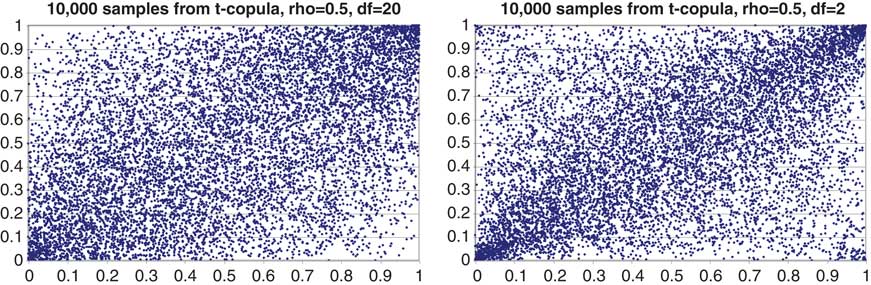
Figure 17 t copula simulations (rho = 0.5, df = 20 and df = 2).

8.5.4 Gumbel Copula

8.5.4.1 The Gumbel family of copulas is given by the formula:

By substituting this expression into the formula for the coefficient of tail dependence we get:

8.5.4.2 Figure 18 shows simulations from a 2-dimensional Gumbel copula with the parameters:

Figure 18 Gumbel copula simulations (theta = 2 and theta = 4).

1. (i) theta = 2; and

2. (ii) theta = 4.

It is clear from the second graph that the copula with theta = 4 has a higher upper tail dependence.

8.5.5 Clayton Copula

8.5.5.1 The Clayton family of copulas is given by the formula:

8.5.5.2 Figure 19 shows simulations from a 2-dimensional Clayton copula with the parameters:

Figure 19 Clayton copula simulations (theta = 2 and theta = 10).

1. (i) theta = 2; and

2. (ii) theta = 10.

It is clear from the second graph that the copula with theta = 10 has a higher lower tail dependence.

8.6 Copula Selection

8.6.1 At the moment, the most commonly used copula in economic capital modelling is the Gaussian copula. It is relatively easy to understand, mathematically tractable and can be programmed easily to generate simulated output within an economic capital model. A limitation is that it does not induce tail dependency for extreme losses.

8.6.2 A natural progression on from the Gaussian copula is to consider the use of other copulas such as the t copula, or those from the Archimedean copula family such as the Gumbel, Clayton and Frank copulas.

8.6.3 In economic capital modelling we are of the opinion that the most obvious copula to investigate beyond the use of the Gaussian copula is the t copula (and later its extension the Individuated T (‘IT’) copula). Even with the use of the t copula there still remains the issue of determining both the:

1. (i) correlation matrix; and

2. (ii) tail dependency parameter,

so as to produce results, that give the requisite tail dependency at high loss percentiles.

8.7 Parameterisation

8.7.1 The practical issues arising when trying to estimate a correlation coefficient from real data were highlighted in section 7.5. With the parameterisation of copulas there is a further issue of how to parameterise the factors that determine the degree of tail dependency between risks in extreme loss scenarios.

8.7.2 For the t copula (or its IT copula extension) one has to estimate degrees-of-freedom parameters, whether it is just one parameter as for the more straightforward t-copula, or n parameters for the more complex IT-copula. One way of doing this is to estimate the tail dependencies for each pair of risk factors from historical data or expert opinion/judgement, and then use an iterative algorithm which finds the set of degrees-of-freedom parameters implying the closest possible tail dependencies using the approaches described later in this section.

8.7.3 If we aim to model tail dependency more accurately, whichever type of copula we are using, we will need to estimate extra parameters which influence the tail dependency.

8.7.4 Estimating copula parameters needs good quality data. Problems arising include, however it should be noted that the first three are not necessarily unique to copulas:

• – Data may not be available, and if available, either of poor quality or incomplete. Asset related data such as returns for equity and fixed interest rate risk are generally more readily available and homogenous than some of the data related to insurance line of business related risks.

• – Data may be sparse due to the low frequency of the risk.

• – The frequency of the data will also be dependent on the nature of the risks. Asset related time series data is available at least daily whereas insurance loss data may typically only be available on either quarterly or annually

• – If we try to estimate parameters from real data, then we are going to have to use data from economic periods where extreme events occurred and by definition these very low frequency events are scarce data sets.

• – Managing the difficult trade-off of having a long enough historical time series to be representative of such events versus the potential secular risk arising.

8.7.5 There are two general approaches to estimating copula parameters from a data set. These methods are described in Embrechts et al. (Reference Embrechts, Frey and McNeil2005). The two main methods are:

• – Maximum Likelihood Estimation.

• – Method of Moments.

8.7.7 Method of Moments

8.7.7.1 The method-of-moments consists of using an empirical estimate of Kendall's tau rank correlation (or alternatively Spearman's rank correlation) to derive an estimate of a copula parameter.

8.7.7.2 This simpler procedure uses sample rank correlation estimates. This method has the advantage that marginal risk distributions do not need to be estimated and, consequently, inference about the copula does not depend on margin assumptions.

8.7.7.3 We illustrate the method by estimating the correlation matrix parameter used for Gaussian and t copulas.

8.7.7.4 Both the Gaussian and t copulas require a linear correlation matrix as an input parameter. This matrix is the linear correlation matrix related to the corresponding multivariate Normal distribution. This means that, if the user is estimating the correlation parameters from sample data, then most likely the estimated correlation coefficient will be different from that required as input to the Gaussian and t copulas to perform Monte Carlo simulation, unless that is we assume that the marginal risk distributions being used are normally distributed.

8.7.7.5 The theoretically correct approach for Monte Carlo simulation is to calculate the Kendall tau correlation coefficients between risks from sample data and then to convert these into linear correlation parameters using the following formula, see Embrechts et al. (Reference Embrechts, Frey and McNeil2005):

This formula works for any elliptical copula, of which the Gaussian and t-copulas are the most notable.

8.7.7.6 In practice, if sample data arises from marginal risk distributions related to the Normal distribution family such as the Student t, Chi Squared, Gamma and Lognormal distributions then the estimated correlation parameters ρ_Gaussian are generally quite close to the estimated linear correlation coefficients from the sample data.

8.7.7.7 However, the Pareto, Burr and Cauchy distributions are examples of marginal risk distributions where the estimated correlation parameters ρ_Gaussian are very different to the estimated linear correlation coefficients from the sample data.

Figure 20 shows the correlation parameters sampled from two-dimensional distributions using a Gaussian copula with various marginal distributions.

Figure 20 Correlations using Gaussian copula and various marginal risk distributions.

8.8 Monte Carlo Simulation

This section illustrates, through the use of a case study, the impact of different correlation and dependency structures on the economic capital modelling results of a hypothetical insurance organisation ABC Insurance Company.

8.8.2 Risk Distributions

Table 9 lists the risk categories and the parameters of the risk distributions.

Table 9 Risk distribution assumptions.

8.8.3 Modelling Assumptions

8.8.3.1 The modelling results are shown for four different copulas, namely:

• – Gaussian Copula

• – t Copula with 10, 5 and 2 degrees of freedom (d.f.)

• – Furthermore, economic capital numbers are also shown using the variance-covariance matrix approach (V CV) to risk aggregation

• – Results are shown at varying percentiles ranging from 75% to 99.95%

• – Economic capital is based on a Value at Risk (VaR) risk measure over 12-months and Capital = Loss (%) – E(Loss)Footnote 8 Footnote 9

• – Copula simulation results are based on 25,000 simulations for each copula.

• – Losses are additive.

8.8.3.2 The copula simulation exercise has been performed using the Matlab software from The Mathworks (2009). The Monte Carlo simulation of correlated U(0,1) values of risks for the Gaussian and t copulas within Matlab take as input linear correlation coefficients.

8.8.3.3 Correlation Matrix

Figure 21 shows the correlation matrix with a correlation of 25% between risks.

Figure 21 Correlation Matrix.

8.8.4 Modelling Results

The results of this modelling exercise are discussed in sections 8.8.5 to 8.8.7.

8.8.5 Lognormal risks (CV = 25%, Correlation = 25%)

8.8.5.1 In Table 10 the economic capital results for the t copula and the variance-covariance matrix approaches have been expressed as percentage changes +/− % of the economic capital of the Gaussian copula, e.g. at 99% the economic capital using the t copula with 5 d.f. (8,177) is 10.2% higher than the Gaussian copula at the same percentile (7,423).

Table 10 Lognormal risks (CV = 25%, Correlation = 25%).

8.8.5.2 Note: The variance-covariance matrix calculation uses a linear correlation matrix consistent with the 25,000 simulated lognormal outputs for each risk within each of the four different copula simulations runs. In fact the average correlations of the 45 (=10.(10−1)/2) pairs were 24.1%, 24.6%, 25.0% and 25.3% respectively for each of the Gaussian copula, t copula (10 df), t copula (5 df) and t copula (2 df). Using 25% in the variance-covariance matrix calculation is therefore consistent.

8.8.5.3 Comments of note are:

• – If we consider the Gaussian copula as our reference point then quite clearly there is a very wide range of outcomes depending on the approach used to aggregate risks.

• – When the marginal risk distributions are non-normally distributed and positively skewed, then at higher percentiles the V CV capital approach to capital aggregation gives larger economic capital values than use of the Gaussian copula.

• – With lognormal marginal risk distributions, the variance-covariance matrix approach to economic capital at the higher percentiles produces similar capital to a t copula with appropriate degrees of freedom. For example at 99% the V CV economic capital is 8,212 which is marginally larger than the economic capital of 8,177 arising from the use of a t copula with 5 d.f.

• – As the percentile increases, the larger the implied d.f for the t copula (lower tail dependency) to give the equivalent level of economic capital as the V CV approach.

8.8.5.4 Appendix E provides the same exhibit as above but shows the sensitivity of the results to different correlation coefficients. Results are shown for correlations of 10%, 25% and 50%.

8.8.6 Lognormal risks (CV = 25% and 50%, Correlation = 25%)

8.8.6.1 A natural question to ask is the sensitivity of the economic capital to variation in the CV of the underlying marginal risk distributions. In Table 11 the CV of the Lognormal distribution has been increased from 25% to 50%.

Table 11 Lognormal risks (CV = 25% and 50%, Correlation = 25%)

8.8.6.2 Again, as in section 8.8.5 the economic capital in the tables is expressed as percentage changes +/− % of the economic capital of the Gaussian copula.

8.8.6.3 Comments of note are:

• – At the higher percentiles, 95% and above, a larger CV results in larger percentage increases of V CV economic capital compared to the Gaussian copula.

• – Furthermore, with a higher CV the equivalent t copula implied d.f. such that the capital is equivalent to that of the V CV approach are lower (i.e. greater tail dependency). For example, at 99% with a CV of 25% the V CV approach is similar to a t copula with 5 d.f. whereas with a CV of 50% the V CV approach looks to be similar to a t Copula with a d.f. about half-way between 2 and 5 d.f.

8.8.7 Normal vs Lognormal risks (CV = 25%, Correlation = 25%)

8.8.7.1 In Table 12 the analysis here considers the sensitivity of the economic capital results to variation in the assumed marginal risk distributions. A comparison has been made of the results arising from use of the Normal distribution compared to those arising from use of the Lognormal distribution as used in the prior sections.

Table 12 Normal vs Lognormal risks (CV = 25%, Correlation = 25%).

8.8.7.2 Again, as in sections 8.8.5 and 8.8.6 the economic capital in the tables is expressed as percentage changes +/− % of the economic capital of the Gaussian copula.

8.8.7.3 Note: For the Normal distribution the variance-covariance matrix calculation uses a linear correlation matrix consistent with the 25,000 simulated normal outputs for each risk. The average correlations were 24.7%, 24.1%, 24.7% and 24.8% respectively for each of the Gaussian copula, t copula (10 df), t copula (5 df) and t copula (2 df). Using 25% in the variance-covariance matrix calculation is therefore consistent.

8.8.7.4 Comments of note are:

• – When the marginal risks distributions are Normal then the V CV approach to capital aggregation should give equivalent economic capital results to those of the Gaussian copula.

• – The last column in the top table above shows percentage value differences that are nearly, but not exactly equal to 0%. Any differences from 0% being due to simulation error, even with 25,000 simulations.

9.1 What Do We Mean by Tail Dependency

9.1.1 The overriding deficiency of all types of correlations that we have described in Section 4, namely linear and rank correlation, is that they are only scalar measures of dependency and do not allow us to model how dependency changes with economic circumstances.

9.1.2 For example, they do not allow us to model dependency between risks conditional on the underlying values of the risks themselves, which is often a feature of actual events be it the recent financial crisis or natural disasters such as earthquakes or hurricanes where the observed dependency between risks tends to increase in the event of such scenarios.

9.1.3 A feature of tail dependency is that one extreme event or series of events will trigger risks that are normally assumed to be independent or otherwise have low correlation.

9.1.4 Turning to the insurance industry, it is recognised that very large events can trigger multiple lines of business. The 9/11 World Trade Centre attack is a prime example of this where large insurance loss amounts were seen in property, business interruption, marine, workers compensation and life insurance lines of business. However, this was not the end of the losses as the consequences included falling asset values on insurer's balance sheets.

9.1.5 The recent financial crisis has had huge impact across all financial markets. A standard observed pattern of relatively low levels of dependency between various financial asset classes, such as equities, fixed income, credit risk and foreign exchange rates was replaced by severe losses occurring at the same across all markets. Dependency empirically observed in the market at a time of extremely bad economic conditions (tail dependence) tends to differ structurally from the dependency levels observed in normal market circumstances.

9.1.6 Figure 24 illustrates this idea. It shows the annual returns of two stock market indices: S&P500 and Nikkei 225 in each month for the last 40 years.

Figure 24 S&P 500 vs Nikkei 225 returns.

9.1.7 We can see from Figure 24 that in benign markets, when the values of the two indices are highly positive, the correlation between them is relatively weak (the points on the RHS are quite widely spread). But in adverse conditions, when the returns are highly negative, the correlation is relatively larger (the points on the LHS form much more of a concentrated pattern). In fact, the linear correlation coefficient calculated for all months when the S&P500 return was negative was 0.9, whereas the linear correlation coefficient calculated for all months when the S&P500 return was positive was 0.4.

9.1.8 The challenge of a good economic capital model is to capture the main features of complex and unpredictable relationships between multiple real world risks with relatively simple mathematical structures. Any differences between the model and reality are accentuated in times of stress.

9.2 The So-Called ‘Tail Correlation’

9.2.1 A common approach used by some insurance companies to reflect tail dependency when performing a variance-covariance matrix economic capital calculation is to use correlations that are larger than an average correlation that has been estimated from empirical data in normal market conditions.

9.2.2 The concept of a so-called ‘tail correlation’ appears to have gained currency in describing such a correlation coefficient.

9.2.3 To quote from the International Actuarial Association's (2004) paper “A Global Framework for Insurer Solvency Assessment”

9.2.4 Elsewhere the concept has appeared under a different guise, none more than so in the various CEIOPS Solvency II consultation papers on the deduction of the correlation coefficients for use in the risk aggregation process within the SCR Standard Formula. The latest version of which is CEIOPS (2010c).

9.2.5 For example, within section 3.1 (page 7) of this paper is stated:

9.2.6 However, we feel obliged to point out that that such a correlation to reflect ‘tail’ dependency between two risks X and Y is not adequately described by the relationship in section 3.20 (page 11). In fact this formula, namely:

where F_X and F_Y are the distribution functions of X and Y respectively,

describes the right tail concentration function which is a completely different measure to the linear correlation coefficient. This function is discussed further in section 11.6 of this paper.

9.2.7 The use of higher correlations to reflect tail dependency is a practical, transparent and intuitive method that will result in economic capital being larger than would be the case from using ‘average’ correlations assessed in normal market conditions.

9.2.8 However there are certain theoretical shortcomings when higher correlations are used in conjunction with the variance-covariance matrix approach to capital aggregation:

• – Higher correlations do not model tail dependency. Tail dependency is a measure of dependence between the risk factors defined using a limit. For example, if you use a Gaussian copula, its tail dependence will be zero irrespective of whether you are using higher correlation parameters or not.

• – There are usually no theoretical foundations for their selected values.

• – The ‘tail correlation’ to be used is not only dependent on the risk measure of interest but also on the nature of the underlying marginal risk distributions, especially when risks are not normally distributed.

9.2.9 An alternative approach which would allow companies to get around these difficulties would be to use a copula with positive tail dependency, such as a t-copula. However, owing to the issues surrounding copulas, mainly in the area of parameterisation, in reality many companies are currently using higher than average correlations, or ‘tail correlations’, to reflect views about tail dependence. Such selections are often done on the basis of a prudent margin.

9.2.10 We shall see in the next section 9.3, that the requisite ‘tail correlation's to be used to combine capital amounts can be much lower than would be expected and on many occasions the resulting coefficients can appear to be counterintuitive.

9.3 Use of ‘Tail Correlations’ Instead of Tail Dependence

9.3.1 If we accept that a t copula with n degrees of freedom induces tail dependency at the loss percentiles often used in economic capital modelling, then a question to ask is:

9.3.2 Mathematically we have calculated the effective linear correlation coefficient x% such that: Variance-covariance capital (using x%) = Copula capital (using 25% correlation, t copula with n d.f.) at any given percentile.

The results are shown in Tables 13–16.

Table 13 Economic Capital Results as per table 10.

Table 14 Implied linear correlation coefficients x% using table 13 data.

Table 15 Economic Capital Results for Normal risks used to derive table 12.

Table 16 Implied linear correlation coefficients x% using table 15 data.

10.1 Methodology

10.1.1 As noted in section 5.7, this method is intuitively very appealing as it can reflect directly, more than any other methods, possible relationships that might exist between different risks. The method can be describe as the simulation of common risks, for every risk, instead of modelling each risk separately and then aggregating them into a joint loss distribution. The economic capital model implicitly captures any diversification benefits between risks.

10.1.2 Within the causal modelling approach the risk dependencies are likely to be at a more granular level than one would see within the variance-covariance matrix approach. For example, some typical causal models capture dependencies such as:

• – Rate movements between lines of business.

• – Large loss frequency between lines of business.

• – Inflationary link between loss reserves and loss volatility.

• – Inflationary link between loss reserves and asset values.

10.2 Some Examples

10.2.2 Simple CDO Model

10.2.2.1 A simple example of thinking of dependencies is where the value of a risk in any given scenario is made up of the impact from a set of simulated common risk factor drivers plus a simulated residual component for that risk. Furthermore, the residual components may themselves be subject to correlation.

10.2.2.2 In simplified forms of Collateralised Debt Obligation (CDO) modelling it was common to assume the latent variable was the asset return of a counterparty. Default was deemed to occur when the value of the counterparty's asset return in any particular scenario fell below some ‘asset’ threshold, itself related to the value of its liabilities.

10.2.2.3 One could represent the asset return for each counterparty as a multi-factor model.

10.2.2.4 In the simplest case we will consider a 2 factor model which consists of a:

1. (i) systematic component; and

2. (ii) non-systematic part.

10.2.2.5 Let the systematic component X be the “state of the economy”, the “counterparty asset return correlation with the market” and ε_i the counterparty-specific (or residual risk) part. It is further assumed that the variables X and ε_i are normally distributed. In this example X is the underlying common risk driver, with the values of R_i and ε_i also determining the degree of dependency between risks.

For each counterparty i = 1 and 2 the asset return can be defined as:

Furthermore, given AR₁ and AR₂ the asset correlation ρ_A is then:

Example: = 50% and = 20% then ρ_A = 15.81%

The R² represents the proportion of the asset return that can be explained by variation in the state of the economy i.e. systematic risk. The non-systematic part consists of both counterparty specific pieces and non-counterparty specific pieces that are common to groups of credit assets but are not deemed to be systematic in natures. The R² can be determined for a company by computing the correlation of the asset value of the company with an index of asset values that represents the universe of companies.

10.3 Advantages and Disadvantages of Causal Model Approach

Advantages

• – Theoretically it is a very appealing and intuitive method.

• – Potentially the most accurate in imitating the way the ‘real world’ works with a series of external and internal shocks to a company.

• – Could be used in combination with other methods, e.g. an inflation variable may be used as a common risk driver for expense and claims risks with some further correlation between the expense and claims risks due to other factors.

• – Possible to capture non-linearities through causal risk relationships.

Disadvantages

• – Transparency and results communication becomes an issue – ‘Black Box’ approach.

• – Parameterisation issues relating to the causal relationships.

• – Could lead to an overly complicated model providing a false sense of accuracy.

• – The most demanding in terms of inputs.

• – It is not feasible to model all common risk factors at the lowest level.

• – If lots of common risk factors are simulated using a Monte Carlo approach, this puts a very high demand on computing power.

10.4 Causal Modelling Design Challenges

There are some additional design challenges for insurance companies contemplating using causal models, or ‘integrated models’ using Solvency II nomenclature.

11.1 Different Ways of Thinking About Dependency

11.1.1 One of the key challenges facing organisations is how to communicate the effect of dependency modelling on the economic capital results to senior management and other non-technical audiences.

11.1.2 With the prospect of many insurance companies applying for internal model approval for 2012 under the Solvency II regime, the importance of communication on such matters is of particular importance, given that under the Use Test requirement:

• – Senior management, including the administrative or management body shall be able to demonstrate understanding of the internal model and how this fits with their business model and risk-management framework.

• – Senior management, including the administrative or management body shall be able to demonstrate understanding of the limitations of the internal model and that they take account of these limitations in their decision-making.

11.1.3 This section therefore describes some simple measures that could be adopted by firms in their communication either internally to the board of directors and senior management or externally to various stakeholders.

11.1.4 Furthermore, the values of the metrics arising from the application of specific copulas can be compared with the values of the same metrics computed from empirical data to help determine the most appropriate copula for the data under study.

11.1.5 For the sake of simplicity, we shall continue with the use of ABC Insurance Company to illustrate the calculations for each of the measures of interest.

11.1.6 The following is a list of possible measures. It is not exhaustive but illustrative of different approaches, some more complex than others:

• – Economic Capital Aggregation.

• – Joint Probability Density Function.

• – Scatter Plot.

• – Joint Excess Probability.

• – Tail Concentration Function.

• – Kendall Tau Correlation.

• – Coefficient of Tail Dependence.

• – Implied Gaussian Correlation.

11.1.7 There are three possible levels of data granularity:

• – Comparisons made at an aggregate level e.g. total Economic Capital.

• – Comparisons made between a pair of risks e.g. “Scatter Plot”.

• – Comparisons made between all risk pairs e.g. “Tail Concentration Function”

11.1.8 The numerical exhibits that follow are based on simulated Matlab output with the same underlying assumptions as listed within section 8.8 for the 10 risk categories of ABC Insurance Company. In the sections where graphical results are shown for two risks, say X and Y, there are two options, (i) actual values of x,y from the distributions of X and Y respectively or (ii) values of u,v such that F_X(x) = u and F_Y(y) = v for X and Y respectively. In most cases the presentation format of (ii) has been adopted. Also, unless otherwise stated e.g. in section 11.2 “Economic Capital Aggregation”, the output from a t copula with 5 d.f. has been used.

11.2 Economic Capital Aggregation

Description

The objective here is to calculate the total economic capital at the different percentiles using a number of different risk aggregation techniques. In Figure 25 capital numbers are shown for the:

Figure 25 Economic Capital Results using different methods (as per Table 10).

1. (i) Gaussian copula

2. (ii) t Copula at 10, 5 and 2 d.f.; and

3. (iii) variance-covariance matrix approach to capital aggregation.

Exhibit

Advantages

• – It is relatively simple to understand.

• – It is possible to directly measure the financial impact on a company.

Disadvantages

• – One has no information of what is happening at an individual risk category level at each percentile of interest.

• – The calculations are more computer intensive than those that will be discussed in the following sections.

11.3 Joint Probability Density Function

Description

The Joint Probability Density function is a three dimensional representation of the plot of the values from two risk factor distributions, in Figure 26 risks X1 and X2. A greater density of points represented by a larger value of the PDF.

Figure 26 Joint Probability Density Function for two risks.

Exhibit

Advantages

• – It is relatively simple to understand.

• – The exhibits are relatively easy to create.

Disadvantages

• – Simulation error may distort the presence or otherwise of ‘tail’ dependency strength.

• – There is no numerical measure that reflects the degree of dependency between risks.

• – One can only use this method for a pair of risks at a time.

11.4 Scatter Plot

Description

A scatter plot involves a plot of the joint values simulated from two risk distributions. In this example the values (u,v) corresponding to amounts x and y from risk distributions X and Y have been plotted. Furthermore, u and v are defined by the relationships F_X(x) = u and F_Y(y) = v, where u and v are values on the interval [0,1].

The extent of the clustering of points in the region of (1,1) indicates the level of ‘tail’ dependency between two risks.

In the exhibits that follow within this section and sections 11.5 to 11.9 we have used risk category names of ABC Insurance e.g. UW Non-Cat and Interest Rate as is the case in Figure 27.

Figure 27 Scatter Plot for two risks.

Exhibit

Advantages

• – It is relatively simple to understand.

• – The exhibits are very easy to create.

Disadvantages

• – Simulation error may distort the presence or otherwise of ‘tail’ dependency strength.

• – There is no numerical measure that reflects the degree of dependency between risks.

• – It may be difficult to distinguish a pair or risks with higher tail dependence from a pair of risks with higher correlation but lower tail dependence.

• – One can only use this method for a pair of risks at a time.

11.5 Joint Excess Probability

Description

For a pair of risks, the Joint Excess Probability is the joint probability that 2 risks are either greater or lower than some deemed threshold. Notation wise:

• ▪ RJEP(z) = P(u > z, v > z)Footnote 11

• ▪ LJEP(z) = P(u < z, v < z)

where: u and v are defined by F_X(x) = u and F_Y(y) = v; x and y are values from X and Y respectively and u and v are values on the unit interval [0,1].

For independence the values of RJEP(z) and LJEP(z) are (1-z)² and z² respectively.

Exhibit

Figure 28 is an illustration of the RJEP(z) concept using a scatter plot of the simulation output for two hypothetical risks X and Y.

Figure 28 Calculation of RJEP(z) for z = 0.8.

e.g. RJEP(0.8) = No. of Points in A/Total No. of Points (in this case 1,000).

11.5.1 Figure 29 is a matrix of values of the function RJEP(0.95) for each of the pairwise combinations of the 10 risks.Footnote 12

Figure 29 Matrix of values of RJEP(z) for z = 0.95.

11.5.2 For comparative purposes the value of RJEP(0.95) = 0.25% is shown where risks are independent of each other, i.e. there is 0% correlation.

11.5.3 In the example illustrated in Figure 29, the values between risk pairs should be identical however the presence of simulation error leads to small differences. With different pairwise correlations between risks the matrix of values becomes more meaningful.

Advantages

• – It is practical and the concept is relatively easy to understand.

• – The calculation is relatively easy to perform.

• – It allows the quantification of the level of dependence at a given percentile in a way which is both mathematically tractable, and simple to understand.

• – It provides a consistent methodology for comparing the relative strength of dependency between two or more risks whether the dependence between them is expressed using copulas or correlations, or in any other way.

• – For more than two risks it is possible to estimate RJEP(z) and LJEP(z) for each pair of risks and present the information as a matrix of values for all risks or a pair of risks.

Disadvantages

• – For most of practitioners used to linear correlations this would be a new concept and some confusion between the two numbers is possible. In particular, it could be mistaken to be a ‘tail correlation’, i.e. the level of correlation in the tail. In fact, the RJEP(z) and LJEP(z) functions are probabilities, i.e. take values between 0 and 1 whereas a correlation coefficient takes values between −1 and 1.

• – It is difficult to translate a value of RJEP(z) or LJEP(z) into a number that is commonly understood e.g. linear correlation, or its equivalent at the ‘tails’.

• – Simulation error may distort the presence or otherwise of ‘tail’ dependency strength.

11.6 Tail Concentration Function

Description

For a pair of risks, the strength of ‘tail’ dependence between risk factors can be defined using the Right and Left Tail Concentration Functions R(z) and L(z) respectively as follows:

• – Right Tail Concentration Function: R(z) = P(u > z / v > z) = P(u > z, v > z) / P (v > z)

• – Left Tail Concentration Function: L(z) = P(u < z / v < z) = P(u < z, v < z) / P (v < z)

where: u and v are defined by F_X(x) = u and F_Y(y) = v; x and y are values from X and Y respectively and u and v are values on the unit interval [0,1].

Technically speaking, if we have more than two risks, e.g. three risks, then R(z) should be defined as R(z) = P(u > z/v > z, w > z) etc.

Exhibit

Figure 30 is an illustration of the R(z) concept using a scatter plot of the simulation output for two hypothetical risks X and Y.

Figure 30 Calculation of R(z) for z = 0.8.

e.g. R(0.8) = No. of Points in A / ( Total No. of Points (A + B))

11.6.1 Figure 31 is a matrix of values of the function R(0.95) for each of the pairwise combinations of the 10 risks.Footnote 13 In this example the values between risk pairs should be identical however the presence of simulation error leads to small differences. With different pairwise correlations between risks the matrix of values becomes more meaningful.

Figure 31 Matrix of values of R(z) for z = 0.95.

11.6.2 For comparative purposes the value of R(0.95) = 5.0% is shown where risks are independent of each other, i.e. there is 0% correlation.

Advantages

• – It is practical and the concept is relatively easy to understand

• – The calculation is relatively easy to perform

• – It allows the quantification of the level of dependence at a given percentile in a way which is both mathematically tractable, and simple to understand

• – It is closely linked to another important copula parameter: “Coefficient of Tail Dependence” (section 11.8) which is a limiting case of the tail concentration function

• – It provides a consistent methodology for comparing the relative strength of dependency between two or more risks whether the dependence between them is expressed using copulas or correlations, or in any other way

• – For more than two risks it is possible to estimate R(z) and L(z) for each pair of risks and present the information as a matrix of values for all risks or a pair of risks

Disadvantages

• – For most of practitioners used to linear correlations this would be a new concept and some confusion between the two numbers is possible. In particular, it could be misunderstood to be a ‘tail correlation’, i.e. the level of correlation in the tail. In fact, the tail concentration functions are different mathematical objects: they are probabilities, i.e. take values between 0 and 1 whereas correlation coefficient takes values between −1 and 1.

• – It is difficult to translate a value of R(z) or L(z) into a number that is commonly understood i.e. linear correlation

• – Simulation error may distort the presence or otherwise of ‘tail’ dependency strength

11.6.3 For comparative purposes, the tables of matrices for R(0.95) and RJEP(0.95) are shown for both the T Copula with 5 d.f. and the Gaussian Copula in Appendix G.

11.7 Kendall Tau Correlation

11.7.1 The concept and definition of the Kendall tau rank correlation (or simply the Kendall tau) was discussed in section 4.5.

11.7.2 It is a type of rank correlation, i.e. a correlation coefficient which depends on the ranking of data points, not on their values. Its values lie between −1 and 1.

11.7.3 In the example in Figure 32 the values between risk pairs should be identical however the presence of simulation error leads to small differences. With different pairwise correlations between risks the matrix of values becomes more meaningful.

Figure 32 Matrix of values of Kendall Tau.

Exhibit

Advantages

• – It is intuitively simple and the concept is relatively easy to understand.

• – It is more intuitive to someone who is used to regular linear correlations than other measures such as tail dependence

• – It does not depend on the absolute value of observations, which means it should be better dealing with data outliers.

• – It provides a consistent methodology for comparing the relative strength of two or more different random variables with any type of dependency structure.

• – It is possible to represent the information either as a matrix of values for all risks or a pair of risks.

Disadvantages

• – The calculation is slightly more challenging than with other methods

• – It is difficult to translate values of Kendall Tau into numbers that are commonly understood e.g. linear correlation, or its equivalent at the ‘tails’.

• – It does not identify trends like an ever-increasing “strength of relationship” with an increasing percentile, i.e. it is just a scalar measure, like the linear correlation, so not helpful when modelling tail dependence.

11.7.4 Kendall Tau matrices are shown for both the t Copula with 5 d.f. and the Gaussian Copula in Appendix H.

11.8 Coefficient of Tail Dependence

Description

Like many other concepts in this paper, the concept of tail dependency can be simple and intuitive. We have two random variables, X and Y. If X takes the 99.5^th percentile value, what is the probability that Y also takes a value from the 99.5^th percentile? Tail dependence is the probability that one risk factor is extremely large, given that the other one is extremely large as well.

11.8.1 The Coefficient of Tail Dependence between two risks is an asymptotic measure of the dependence in the tails of the bivariate distribution (X,Y).

11.8.2 For a multivariate distribution with a Gaussian copula, the tail dependence between any pair of risks is always zero. This is one of the important deficiencies of the Gaussian copula for modelling dependence.

11.8.3 For continuously distributed random variables with the t Copula the Coefficient of Tail Dependence is:

where: ρ is the pairwise correlation coefficient between two risks.

11.8.4 These coefficients can be viewed as the limiting conditional probabilities of the functions R(z) and L(z) respectively (see section 11.6)

Exhibit

For t copulas with 10, 5 and 2 d.f. respectively Table 17 shows values for λ in the case of a 25% pairwise correlation between risks.

Table 17 Coefficient of Tail Dependence.

Advantages

• – This is the most accurate mathematical measure of the “true” tail dependence between two risks.

• – It does not depend on the estimated percentile, it is just one single characteristic of a dependence structure, e.g. copula.

• – It provides a consistent methodology for comparing the relative strength of two or more different copulas.

• – It is possible to represent the information either as a matrix of values for all risks or a pair of risks.

Disadvantages

• – It is a relatively new concept and could be counter-intuitive to those who are just familiar with correlations. Moreover, it could actually be confused for ‘tail correlation’, because λ takes values between 0 and 1 (although correlation can take values between −1 and 1).

• – The values of λ are limiting values and do not reflect an ever-increasing value with an increasing percentile.

• – λ = 0 for Gaussian copula.

• – For the t copula λ is limited by the combination of a degrees of freedom parameter and correlation coefficient. Not all values of λ between 0 and 1 are achievable by fixing one of these two parameters and varying the other. E.g., if you are trying to calibrate a t Copula for two risks with correlation 0.5 and a Coefficient of Tail Dependence of 0.7 by choosing the degrees of freedom parameter, this might not be possible.

• – The values use a closed-form solution which may, unless enough simulations are run, provide inconsistent values with values of R(z) from simulated output

11.9 Implied Gaussian Correlation

Description

This method is really a combination of the methods previously described in sections 11.5 and 11.6 with notable differences:

• – R(z) and RJEP(z) values are shown for more than one percentile

• – R(z) and RJEP(z) values are shown for three different scenarios

  • (i) Independence (where correlation is 0%);

  • (ii) Gaussian copula; and

  • (iii) t copula with 5 d.f.

The latter two, using the relevant correlations used. It should be noted, that any copula can be used in place of the t copula, for such comparisons.

Exhibit

Figure 33 shows the values of R(z) for Interest rate risk vs UW Non-Cat risk assuming a correlation of 25%.

Figure 33 R(z) for different copulas and percentiles.

11.9.1 On inspection it can be seen that the values of R(z) are greater for the t copula in comparison with the Gaussian Copula; which in turn has larger values of R(z) compared to an assumption of independence between the risks. This observation holds for all percentiles. Furthermore the ratio of R(z) (t copula) / R(z) (Gaussian copula) increases with an increasing percentile.

11.9.2 The numbers behind this exhibit can also be used to determine a so-called ‘Implied’ Gaussian correlation between a pair of risks at each percentile. For example, at 99.0% the value of R(z) = 15.96% for the t copula (5 df) and 5.31% for the Gaussian copula assuming a linear correlation of 25%. However, if the linear correlation is increased from 25% to 54% then the value of R(z) at 99.0% with the Gaussian copula now equals the same value of R(z) = 15.96% as before. The intention is that the values of these so-called ‘Implied’ Gaussian correlations can be used to compare and contrast different model outputs. This approach is sensitive to simulation error.

11.9.3 The ‘implied’ Gaussian correlation has similarities to the idea of trying to determine ‘tail correlations’ as discussed in section 9.

Advantages

• – It is very useful to compare the t copula alongside the Gaussian Copula and the scenario of Independence. In this way one can get a feeling for the degree of tail dependency of the t Copula at each percentile.

• – Furthermore, showing values at different percentiles is a useful way of comparing how the relative values between the t Copula and the Gaussian copula change with percentile.

• – It is easy to calculate and technically correct.

• – The exhibits are very easy to generate within a simulation model.

Disadvantages

• – It is difficult to translate values of R(z) and RJEP(z) into numbers that are commonly understood e.g. linear correlation.

• – There are not many data points at the extreme percentiles and so the calculation is very sensitive to any simulation error in the joint distribution output.

• – One can only use this method for a pair of risks at a time.

12.1 Combined Stress Tests and Two-Way Correlations

12.1.1 Firms and regulators have developed a number of new approaches to cope with the complexities of risk aggregation. One of these is the development of combined stress tests, where more than one risk materialises at once. The intention may be to construct combined stress tests at a given level of confidence. This requires a generalisation of the percentile concept to multiple dimensions.

12.1.2 Another area of developing interest has been an examination of dependencies under stressed conditions. Correlations are seen as having increased during the financial crisis, limiting the extent to which firms were able to benefit from diversification in stressed circumstances. These ideas have been implemented in several ways, ranging from a vague sense of caution in correlation assumptions to two-way correlation models where different correlations apply between pairs of risk drivers according to the direction of a firm's exposure to those risks.

12.1.3 Concepts of combined stress tests and two-way correlations do not naturally arise from copula approaches to dependency modelling. For this reason, although combined stress tests and two-way correlations have found favour in practical calculations, these have sometimes appeared to lack sound empirical and statistical foundations.

12.1.4 Tukey's (Reference Tukey1975) description of “half space depth” is a promising mathematical context to describe these new tools. As mathematicians fill the gaps in practitioner lore, it is likely that some existing beliefs will be proved as theorems, others will be found to hold in limited circumstances and yet others may be exposed as false.

12.2 Combined Events at a Given Confidence Level

12.2.1 The capital modelling literature makes frequent references to the concept of a “1-in-200 event”, which is interpreted as an event so serious as to be exceeded with a probability of only 0.005. When dealing with a continuous scalar distribution, there are two “1-in-200” events corresponding to the 0.5% and 99.5% percentiles.

12.2.2 The corresponding concept in multiple dimensions is sometimes called a “combined 1-in-200 event”. Such an event might involve several risks, each at a less extreme that 1-in-200 level individually but somehow equivalent to 1-in-200 taken collectively. It has proved difficult to convert this intuitive concept into mathematics. For example, it might seem logical to use sets of equal probability density to define combined 1-in-200 events, but this technique fails in simple cases such as two independent uniformly distributed risks.

12.2.3 We start with a simple generalisation of the α quantiles, called the “likely one-way stresses”. For a random vector X we construct likely combined stresses by stressing the first component to it's α quantile, and setting other components to their conditional expectations given that the first component takes its α-quantile value. We can construct another likely vector based on the 1−α quantile. Similar constructions give further likely events based on the α and 1−α quantile of the other vector components, in each case setting the unstressed components to their conditional mean given the stressed component.

12.2.4 If, for example, our random vector has 10 dimensions this construction gives 20 “likely” points. This is an obvious generalisation of the one-dimensional case. McNeil & Smith (Reference Mcneil and Smith2009) give an example calculation based on two exponential distributions. In this case, the likely one-way stresses appear as follows in 12.2.5–12.2.8

12.2.5 We wish to connect the one-way stresses to form a loop. The appropriate generalisation is as follows. For an arbitrary random scalar, Y, let q_α(Y) denote the α-quantile. Returning to our random vector X, we define the outer likely set, denoted by Λ₊, by

12.2.6 We can see, on taking u to be plus or minus a basis vector that the likely one-way stresses lie in Λ₊. We refer to Λ₊ as the “outer likely set”. The outer likely set is the boundary of a blob which, at its most extreme points, touches the likely one-way stresses.

12.2.7 What use is the outer likely set? One important result is the sufficient condition for solvency. Suppose that a financial firm has net assets that can be expressed as a linear function a(x) of the risk driver vector X. Suppose also that a(x) ≥ 0 for all x in the outer likely set Λ₊. This is sufficient to ensure Prob{a(x) ≥ 0} ≥ α. In other words, a probabilistic test of financial strength is reduced to a series of deterministic combined stress tests.

12.2.8 The practical problem with the use of outer likely sets, as indeed with any measure of dependency, is parameterisation. A conditional expectation given an extreme event is difficult to calculate from historic data because, even if data is plentiful, there will only be one point at the exact α quantile for each risk driver. If the distribution of X is known analytically, the computation is more straightforward. In the case of elliptically contoured distributions the outer likely set is the boundary of an ellipsoid. Other shapes can also arise; McNeil & Smith (Reference Mcneil and Smith2009) show likely sets based on two independent exponential distributions.

12.3 Two-Sided Correlations

12.3.1 Some recent publications have introduced the notion of two-sided correlations. Sources include the CRO Forum (2009) and CEIOPS (2010c). For example, the CRO forum's document says the following about the correlation between equity and interest rate risk:

12.3.2 In this context, “short in duration” refers to insurers whose assets are shorter than liabilities, and are therefore exposed to a fall in interest rates. “Long in duration” refers to the reverse situation, where a rise in interest rates is the greater threat. The proposal is to use different correlations according to the sign of a firm's interest rate exposure. To complete the picture mathematically, we would need also to construct correlations in respect of equity rise scenarios, giving four-sided correlations.

12.3.3 As most insurers are exposed to an equity fall rather than an equity rise, these additional correlations are mainly of theoretical interest.

12.3.4 The CFO Forum's derivation of this range starts from the observed historic correlations ranging from −29% to +73% depending on choice of market and calibration period. The paper then asserts “the period with the worst correlation observed does not necessarily coincide with the period with the worst shocks. It is therefore not relevant to retain the highest correlation ever observed.” This is apparently the reason for shrinking the proposed range from [−29%, +73%] to [0%,50%]. The final step is to apply whichever end of the range is more prudent, which is why the recommendation depends on the sign of a firm's interest rate exposure.

12.3.5 CEIOPS (2010c) follows the CRO FORUM (2009) recommendation, but with a contrasting rationale. Commenting on the proposed 50%/0% split correlations, CEIOPS (2010c) points to UK interest rate (10 year term, from the Bank of England) and MSCI world equity index data. The data consists of the ratio of equity and interest rates to the values a year earlier, sampled at monthly intervals from January 1970 to January 2010. It is a little odd to compare a sterling interest rate to a dollar denominated index, but in the interest of comparability we have continued to adopt that approach for the purpose of this paper. The data is shown in the scatter plot at Figure 34. Also plotted are some lines separating 10% of the data from 90%. We will use these to construct four-sided correlations.

Figure 34 Annual changes in UK interest rate and MSCI world equity index, monthly intervals (1970–2010).

12.3.6 It would be desirable to consider data over longer periods. We have examined the yield on 2.5% consols, and the equity index based on the FTA all share index of UK shares, back-filled with various predecessor indices from January 1923. The corresponding plot from this data set is shown in Figure 35. The estimated percentiles for equities are broadly similar, while the interest rates were less volatile when measured over the longer period.

Figure 35 Annual changes in UK interest rate and MSCI world equity index, monthly intervals (1923–2010).

12.3.7 We now consider how these charts can be used to construct tail correlations. In section 5 we already saw a formula for aggregate quantiles in the case of elliptically contoured distributions. Letting Y = b.X, we have the formula:

12.3.8 We cannot expect this formula to hold in the general case of non-elliptical distributions. However, in the bivariate case, for particular values of b we can back-solve for the correlation R ₁₂ using the following formulas:

12.3.9 This formula is of little use if either of the b's is close to zero. In that case, the numerator is the difference of two large numbers and the denominator is close to zero, so the ratio is unstable. It is of most use when X ₁ and X ₂ contribute in similar measure to the variability of Y, that is when |b ₁|[q_α(X ₁)−q _1−α(X ₁)] = |b ₂|[q_α(X ₂)−q _1−α(X ₂)].

12.3.10 Some care is required in the interpretation of the signs for b ₁ and b ₂. In the example that follows, we investigate the case α = 0.9, so we are interested in the 90% of a distribution. In this case the variable Y = b.X must be interpreted as a firm's losses or net liabilities. There are four ways in which this can occur, corresponding to the four possible sign combinations of b ₁ and b ₂. We identify those four cases by points of the compass, according to which quadrant contains the point (b ₁,b ₂). Working anticlockwise from the North-East corner, we have the four estimated correlations, which are set out in Table 18.

Table 18 Pearson and Tail Correlations for Equity and Interest Data.

Note: CEIOPS SCR Standard Formula Article 111(d) Correlations ("CP 74").

12.3.11 If the underlying distribution were elliptically contoured then we would expect to get similar estimates of R ₁₂ for each quarter, at least within sampling error. The differences observed in our example give some support to CEIOPS suggestion of split correlations. The relevant quadrants for insurers arise when b ₁ < 0, denoting greater losses in the event of an equity fall. Insurers with long duration should have b ₂ < 0, that is the SW quadrant, while short duration insurers are more concerned with the NW quadrant where b ₂ > 0.

12.3.12 This table shows a number of interesting properties. Firstly, we notice the significantly different results from the longer time period. We might think this is driven by data prior to 1970, but in fact this is not the case. Instead, the negative correlations arise because of the events of the early 1970s, when UK shares collapsed and recovered at the same time as interest rates rose to new heights before falling again. This effect is not evident from the MSCI data set because the UK's experience is dominated by other countries in the index which did not share the UK market's volatility.

12.3.13 While the data set does offer some support for different implied correlations in different quadrants, the variations between quadrants are not dramatic, and this analysis does not offer much empirical support for abandoning simpler methods based on Pearson correlations and elliptical distributions. In particular, we note that the CRO forum and CEIOPS recommend the use of higher correlations in the SW corner relative to NW, while the empirical data suggests the reverse.

12.3.14 Therefore, while the CFO forum and CEIOPS suggest that the classical correlation approach may be insufficiently prudent, our analysis suggests the reverse, that the classical approach is already prudent and firms may reduce their stated capital requirement by more accurate modelling of correlations in the tail.

12.4 Half Space Definitions

12.4.1 We now show how tail correlations can be useful in risk aggregation. This requires some mathematical background. Given a random vector X, a (closed) half-space means a set of the form:

12.4.2 Here, u is a non-zero vector and c is a scalar. Equivalently, a half space is a set bounded by a hyperplane. We note that if u and c are multiplied by the same positive scalar then the half space is unchanged. There is no requirement that a half-space has probability 0.5, and it is entirely possible for one half-space to contain another – simply consider varying c in the definition. The use of half space probabilities is a promising alternative to the use of correlations to describe multivariate distributions.

12.4.3 If the probability of every half space is known, this is enough to identify the multivariate probability of X. To see why this is the case, knowledge of the half-space probabilities allows us to construct the characteristic function of u.X for every u, hence the characteristic function of X itself using Fourier's inversion formula. Calculating these in practice is a formidable numerical task, and we do not recommend it. However, this result can give some comfort that there is no loss of information in using methodologies based on half-space probabilities.

12.4.4 Half spaces are particularly relevant for insurance work because in many cases the regions of solvency or insolvency are half spaces or close approximations thereof. Taking a non-life insurance example, suppose X is a vector of loss ratios, u is a vector of premiums and c denotes the available assets. The solvent region is precisely the half-space H_u,c = {x:u.x ≤ c}.

12.4.5 In life insurance, the solvent region may not be exactly a half-space. This is because the risks interact; liabilities cannot always be expressed algebraically as the sum of an interest effect and an equity effect and a lapse effect and a credit effect. As a result, the solvent region may be bounded by a curved surface rather than a hyperplane.

12.4.6 Different methods of model calibration make use of different reference sets. Model calibration involves equating modelled probabilities of reference sets to historical or judgemental frequencies. If the one of the reference sets happens to coincide with the solvent region then we have to worry only about estimation error for that region. If on the other hand, the solvent region is not the same shape as the reference set, then the choice of model becomes important in linking probabilities from one to the other. The model risk therefore depends on how closely the solvent region approximates the reference sets.

12.4.7 Suppose we are given a choice between half space methods and copula methods. In the former case, the reference sets are half spaces; in the latter case, quadrants. It is an empirical question which of these is closer to a particular insurer's solvent region. However, we consider that in many cases the half-space methods are the least bad option, given that solvent regions seldom exhibit the sharp corners of quadrants.

12.4.8 We can also define an inner likely set, denoted by Λ₋. This is defined as the intersection of all half spaces whose probability is α or more. In mathematical symbols:

12.4.9 This is the envelope of all the lines separating probability α from 1−α. While the outer likely set gives a sufficient condition for capital adequacy, the inner likely set gives a necessary condition. The condition is that a(x) ≥ 0 for all x in the inner likely set Λ₋. Under mathematical convexity conditions, the outer likely set is the boundary of the inner likely set, in which case a(x) ≥ 0 for all x in the inner likely set is both necessary and sufficient for capital adequacy. The construction for the 1970–2010 data set is shown in Figure 36.

Figure 36 90%-ile lines and the inner likely set based on 1970–2010 data.

12.4.10 We can see that the inner likely set is closed and convex, as it is an intersection of closed convex sets. Furthermore, the inner likely set is easy to estimate empirically. Intuitively, the result is a blob which touches the boundaries of probability-α half spaces. We plot this for the equity and interest rate data set below, noting that these are set at the 90% level. We have also plotted the corresponding curve equivalent to the CRO forum and CEIOPS requirement for two-way correlations.

12.4.11 The one-way tests in Figure 37 are based on the 45% equity fall as described in CEIOPS (2010b) and the interest rate stress in which the 10 year rate is multiple by factors of 0.69 in the down stress and 1.42 in the up stress as described in CEIOPS (2010a). This last blob is incomplete because the standard formula specifies tests only in respect of equity falls.

Figure 37 Data-based likely sets and the CEIOPS proposals for Solvency II.

12.4.12 We would naturally expect the 99.5%-ile to produce more extreme events than a 90%-ile. The surprise, however, is in the shape of the likely set for CEIOPS proposal which is strikingly different to that implied by historic data. Figure 37 is a graphical representation of the contrasts in Table 18.