


Illite ‘crystallinity’ (IC) as a parameter of the degree of incipient metamorphism was proposed by Weaver (Reference Weaver and Flawn1961), who used the intensity ratio of the X-ray diffraction (XRD) peak at 10 Å and 10.5 Å. The half-height width or full width at half maximum (FWHM) of the white mica/illite 10 Å peak (‘Kübler index’) was used as the parameter of IC by Kübler (Reference Kübler1967), followed by the use of FWHM of the chlorite 7 Å peak for chlorite ‘crystallinity’ by Árkai (Reference Árkai1991). Kübler and following authors measured FWHM of the 10 Å white mica/illite diffraction peak on the diffraction traces.
FWHM is heavily dependent on the experimental diffractometer settings, notably on the scan rate ω (°2θ/min), the time constant, TC (s) and the angular width of the receiving slit, v (i.e. on the relation of TC to the time width W t of the receiving slit, where W t [s] = 60 × v/ω; for step scanning, on the relation of the step width [°2θ] to the receiving-slit width v [°2θ]).
In Neuchâtel, Kübler used 2°/min and TC = 2 s, with a receiving slit of 0.2 mm/0.067° (TC ≈ W t). At the standard settings of Kisch (Reference Kisch1980), 0.6°/min, TC = 2 s, also with a 0.2 mm/0.067° receiving slit (TC ≈ ¼ × W t), FWHM is ~0.04°Δ2θ narrower than at Kübler's settings.
Traditionally measured directly on the diffraction traces, the FWHM of the 10 Å line is increasingly being determined on fitted profiles using various fitting programs, commonly with split (asymmetric) functions (e.g. Pearson VII [e.g. Warr & Rice, Reference Warr and Rice1994; Kisch & Nijman, Reference Kisch and Nijman2010] and seven-point parabolic, or even the symmetric Pearson VII function [e.g. Battaglia et al., Reference Battaglia, Leoni and Sartori2004]), rather than directly on the diffraction traces. These fitting functions are provided as computer software such as Siemens Diffrac II and Philips APD-10 by XRD manufacturers. They provide accurate peak positions for the muscovite/illite 10 Å peaks, but their FWHM* widths differ significantly from FWHM as measured directly on the XRD traces, usually being notably ‘broader’ (except for the very narrow peaks of muscovite strips, where they are narrower).
However, these authors have not established that they provide the best fits of the peaks in question; in most cases, even the asymmetric Pearson VII function gives a poor fit of the profiles of either peak. An assessment of the correct ‘shape’ of the constituent peaks – including the degree of their asymmetry – is essential for the proper deconvolution of composite 10 Å and 7 Å peaks, such as in removing the contribution of paragonite from the composite 10 Å peaks and of kaolinite and chlorite/smectite mixed layers – including corrensite – from composite 7 Å peaks.
The present study took an empirical approach to the broadening of FWHM* as determined on the fitted peaks with respect to that measured on the fitted profiles by comparing FWHM as manually measured on diffraction profile traces of the muscovite/illite 001 reflections at ~10 Å/8.84°2θ CuKα and the chlorite 002 reflections at ~7.05 Å/12.56°2θ CuKα for a range of peak widths with that as determined using asymmetric Pearson VII and Cauchy (Lorentzian) functions in order to evaluate the differences and their causes.
MATERIALS AND EXPERIMENTAL METHODS
Oriented slides of grain-size fractions (abbreviated OGSF) were prepared from samples collected from the Archaean of the Mosquito Creek Basin, East Pilbara Craton, Western Australia; the Eocene of the Olympos area, northeast Greece; the Phyllite-Quartzite Unit of eastern Crete; and the Devonian of western Norway. The polished-slate standards (abbreviated PSS) are from the Cambro-Silurian Jämtland Supergroup, western central Sweden (Kisch, Reference Kisch1980). Profile traces free of unresolved contributions of reflections of phases such as paragonite and illite-rich illite-smectite (I-S) mixed layers to the 10 Å peaks and kaolinite or chlorite-smectite mixed layers to the 7.05 Å peaks were selected. In addition, the effect of broadening by the presence of minor I-S mixed layers was evaluated by measuring both air-dried and ethylene glycol (EG)-solvated sedimented slides. Illite-rich I-S mixed layers are identified by major differences in FWHM of the 10 Å peaks between air-dried and EG-solvated runs. The presence of kaolinite or corrensite is detected by low-angle basal tails to the 7.05 Å peaks and by the appearance of the kaolinite 002 or corrensite 008 reflections at ~3.57 Å/24.94°2θ CuKα (3.45 Å/25.82°2θ for EG-solvated low-charge corrensite) on the low-angle side of the chlorite 004 reflection (cf. Biscaye, Reference Biscaye1964). Because the I14Å/I7Å intensity ratio of corrensite is ~3 (i.e. much greater than that of chlorite [0.25–0.30]), the presence of subordinate corrensite is also suggested by unusually high I14Å/I7Å ratios, whereas that of kaolinite is suggested by unusually low I14Å/I7Å ratios (<0.25).
The XRD patterns of most samples were obtained by step scanning on the Philips generator 1730/goniometer 1050 with Cu-Kα, normal focus tube, Ni-filter and Xenon proportional detector (PW 1711) at the Department of Geological and Environmental Science, Ben-Gurion University of the Negev, by Ester Shani and Robert Tilden (samples from eastern Crete), using this author's standard settings of slits 1°–0.2 mm–1°, TC = 2 s for scan rate 0.6°2θ/min or TC = 1 s for scan rate 1.2°2θ /min by step scanning with 0.01°2θ steps for the 7–22°2θ range and 0.035°2θ steps for longer 3–34°2θ and 2–70°2θ scans. The samples from the Olympos area, northeast Greece, and the polished-slate and muscovite-strip standards were run on a PanAnalytical Empyrean diffractometer with X'Celerator linear detector, with 0.5 mm and 1 mm scatter slits, without a receiving slit, at the Institute for Nannoscale Science and Technology of the University by Dr Dmitry Mogilyanski with 0.004°2θ steps (0.01°2θ steps for the polished-slate standards). Because the resulting peak widths are narrower by some 0.02°Δ2θ than those obtained by the previous standard conditions (Kisch, Reference Kisch1990; Reference Kisch1991, p. 668), the boundaries of the anchizone equivalent to Kübler's 0.42° and 0.25°Δ2θ are then 0.35° and 0.19°Δ2θ instead of 0.375° and 0.21°Δ2θ. Peak fits using the peak-fitting functions were carried out with program Winfit (Krumm, Reference Krumm1994), selecting asymmetric peaks.
RESULTS
Effects of diffractometer settings on FWHMtrace of the 10 Å white mica peak as measured on the diffraction traces
Using various combinations of scan rates, receiving slits and time constants on a PSS supplied by the late Bernard Kübler, Kisch (Reference Kisch1990) showed that the peak width (FWHMtrace) is constant at the same TC/W t ratio (i.e. for the same TC × scan rate at the same receiving slit); the amount of peak broadening is linear with the increase in TC/W t (Kisch, Reference Kisch1990, fig. 4). The incremental 10 Å peak widths ΔFWHM on five polished-slate and one muscovite-strip standards (i.e. the differences between the peak widths and the standard instrumental settings of 0.6°/min, TC = 2 s) upon increased W t (Kisch, Reference Kisch1990, fig. 2) are largely uniform: ~0.04–0.05°Δ2θ per TC/W t unit on the narrower peaks, with only subordinate additional broadening of the broader peaks by minor amounts of up to 0.005°Δ2θ or 10% of absolute FWHM.
Subsequently, the FWHM values on series of Kisch's standard slabs were measured by a large number of laboratories at their settings; of these, the results of 19 different laboratories/settings are given in Fig. 1.
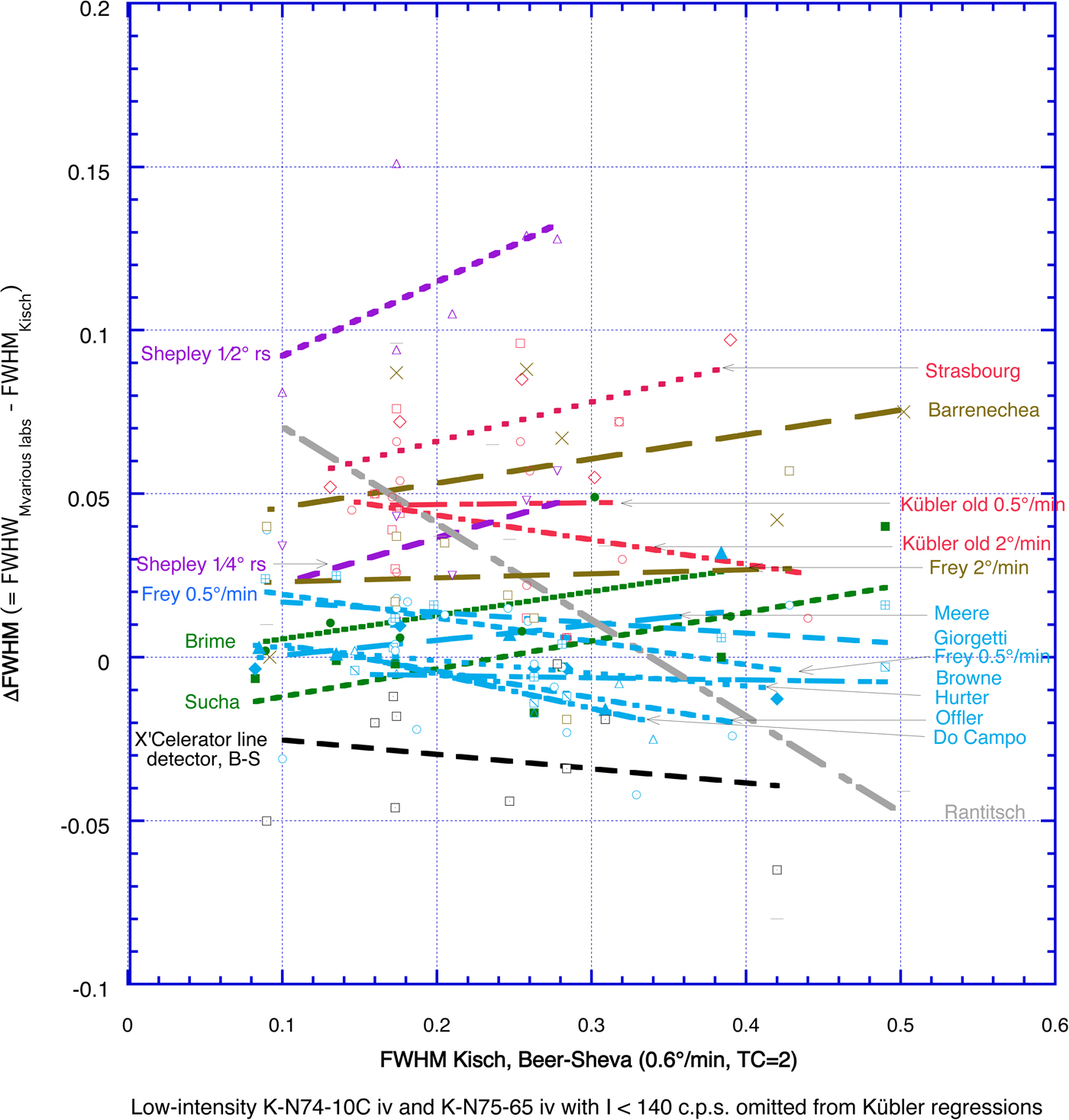
Fig. 1. Difference between FWHMtrace as measured on traces of Kisch's polished-slate standards and muscovite strips by 14 researchers at 18 settings and by Kisch at his standard settings. Regression colours: pale blue – continuous scans with TC/W t ≤¼, receiving slit (r.s.) = 0.2 mm (Giorgetti; Offler; Meere; Do Campo; Frey) and step scans with 0.01° steps, r.s. = 0.2 mm, step width/receiving slit = 0.15 (Browne; Hurter); dark green – step scans with 0.02° steps, r.s. = 0.2 mm, step width/receiving slit = 0.3 mm (Brime; Šuchá); brown – TC/W t = ½, r.s. = 0.2 mm (Barrenechea; Frey); red – TC/W t = 1, r.s. = 0.2 mm (Strasbourg; Kübler 2°/min and 0.5°/min); and purple – large TC, very broad r.s. = ½° or ¾° (Shepley: TC = 3 for 0.5°/min at r.s. of ¼° or ½°, respectively, 0.18° and 0.43° broader than 0.2 mm/0.07°). The contributors and their laboratories are listed in the acknowledgments.
The differences between average FWHMlabs and FWHMKisch (ΔFWHM) increase with increasing TC/W t, step width and receiving slit width. For 0.2 mm (0.067°) receiving slits, the average differences in ΔFWHM are:
(1) –0.015° to +0.015°Δ2θ at small TC/W t ≤ ¼ and step scans with 0.01° steps (pale blue in Fig. 1), with very gentle, mostly negative regression slopes.
(2) Slightly greater, +0.005° to +0.02°Δ2θ, at step scans with 0.02° steps (dark green in Fig. 1), with gentle, positive regression slopes. Woldemichael (Reference Woldemichael1998) reported a similar average FWHM increase of 0.054°Δ2θ upon increasing the step size from 0.01° to 0.03° (i.e. TC/W t from 0.15 to 0.45).
(3) Much larger, +0.04° to +0.08°Δ2θ, at larger TC/W t = ½ (brown in Fig. 1) or 1 (red in Fig. 1), with gentle to moderate positive regression slopes.
For broader receiving slits of ¼° and ½° (purple in Fig. 1 – Shepley), the average differences increase to +0.03°Δ2θ with ¼° receiving slits and as much as 0.11°Δ2θ with ½° receiving slits, with the steepest positive regression slopes found in these instances.
The FWHM values measured on the Philips Empyrean diffractometer with X'Celerator linear detector in Beer-Sheva are, on average, 0.04°Δ2θ narrower than those at standard settings.
The large scatter of the FWHM values for the various laboratories at similar values of TC/W t is not surprising in view of possible aberrant diffractometer linings. Despite this large scatter, the larger increments in FWHM for higher values of TC/W t are in accordance with those found by Kisch (Reference Kisch1990).
Shape of fitting functions and causes of the FWHM broadening
Fits of low-angle 10 Å muscovite/illite 001 reflections with the split (asymmetric) Pearson VII function show poor quality, as is evident from several persistent associated features: (1) insufficient coverage of the ‘tails’ at the base of the peak profiles and reduction of the intensity of the fitted peak by up to 20% with respect to that of the diffraction profile traces; (2) concomitant broadening of the Pearson VII profiles in the middle part of the peaks, resulting in broader FWHM*PVII values by up to 0.05°Δ2θ than those measured on the diffraction profile; and (3) fairly poor reliabilities of the Pearson VII fits – usually between 91% and 97%.
Figures 2–4 give examples of the shapes of some fitted and unfitted profiles of three very different peaks. The XRD traces of most peaks are characterized by both strong upper-peak tapering and sluggish tail fading (e.g. Figs 2, 3). Most fitting functions in use fail to ‘simultaneously’ accommodate both of these features: relative to the traces, they show ‘more rapid’ fading of the proximate peak tails and ‘less tapering’ of the upper peaks. This results in reduced intensity or ‘under-fitting’ of both proximate peak tails and upper peaks and compensatory broadening (‘over-fitting’) of the intermediate curve-fit flanks, where FWHM is measured, most markedly for peaks with ‘both’’ high tails and sharp tops. Additional FWHM* broadening on the fit functions is caused by their reduced intensity, and thus of their half-maximum position, which is located below that of the diffraction traces. Hence, FWHM* is broader. Both effects strongly decrease from Gauss to Pearson VII to Cauchy function fits, reflecting their increasingly sluggish peak-tail fading and more strongly tapered upper peaks. This is also reflected in the increase of their integral breadth (IB)/FWHM ratios from ~1.085 ≈ ½(π – 1) (= 1.071) or ≈½√(π/ln2) (= 1.064) (Gauss), through 1.22 = (π/√2) – 1 (Pearson VII), to 1.57 = ½π (Cauchy), where integral width IB = peak area A divided by the intensity at peak maximum I max.
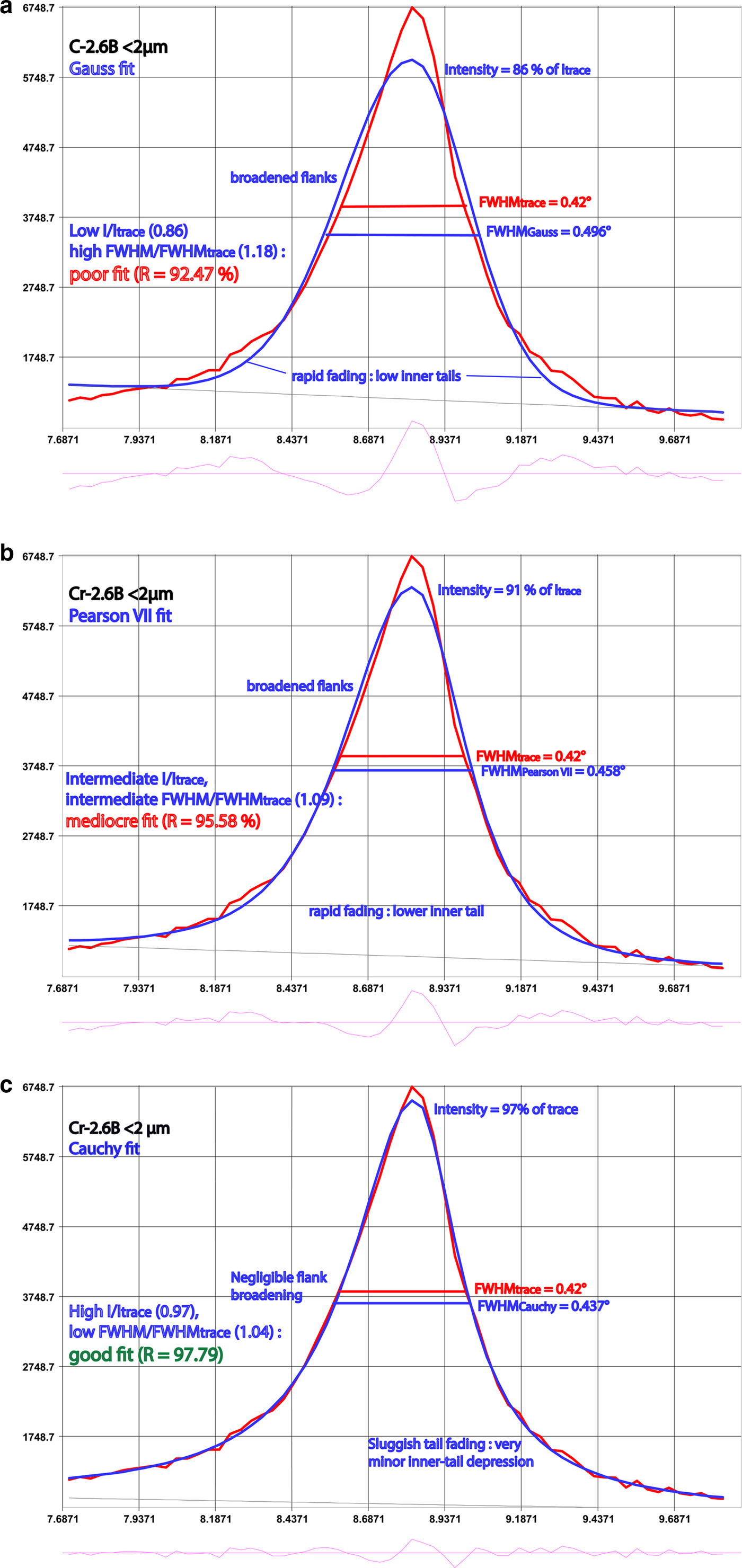
Fig. 2. XRD trace of the Cr-2.6B pipetted slide fitted with Gauss (a), Pearson VII (b) and Cauchy (c) functions.
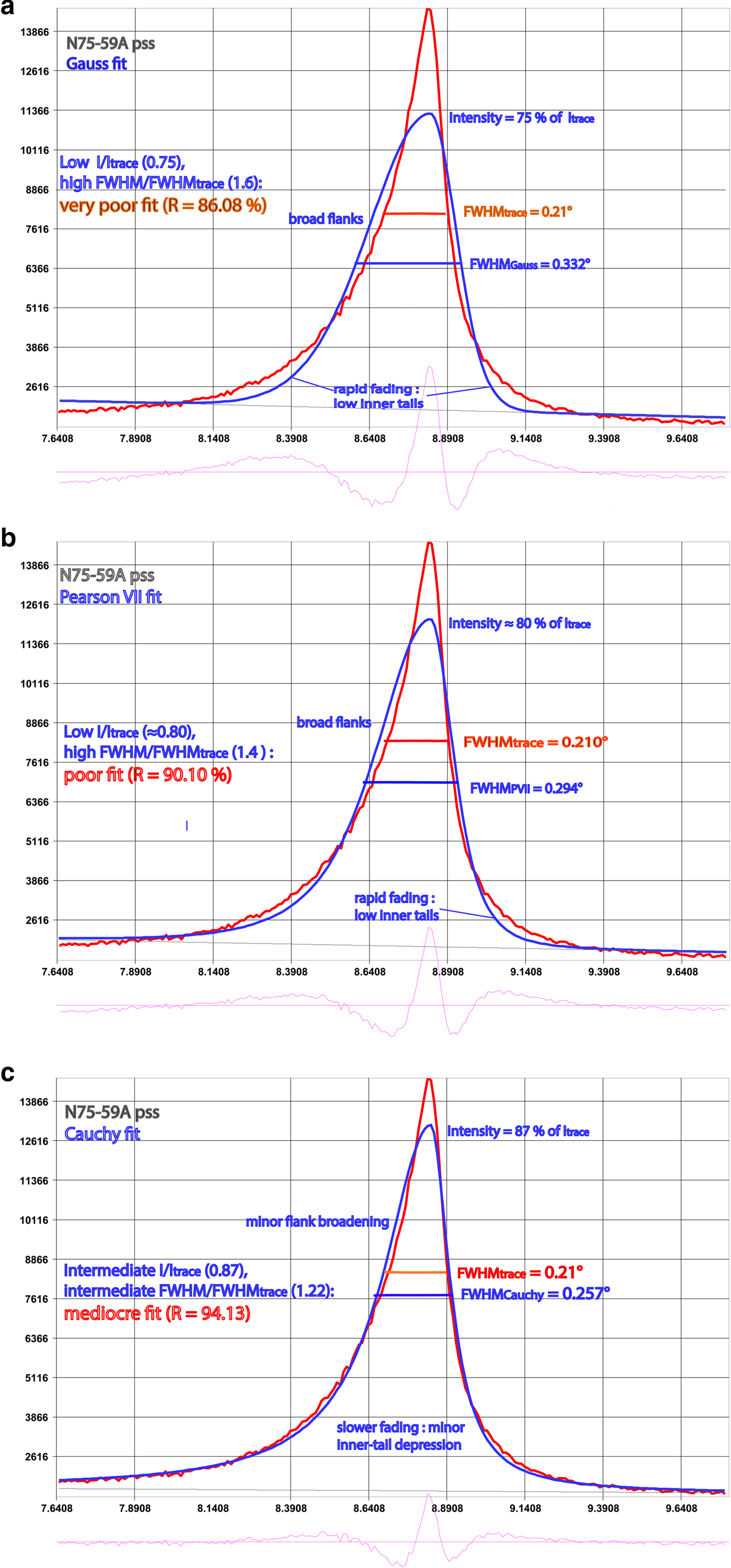
Fig. 3. XRD trace of the N75-59A polished-slate standard fitted with Gauss (a), Pearson VII (b) and Cauchy (c) functions.

Fig. 4. Muscovite strip fitted with the Pearson VII function.
The extent of tapering of the peak top and fading of the peak base is indicated by the Pearson exponent μ and the shape coefficient SC. The Pearson exponents, μ, of the Cauchy, Pearson VII and Gauss functions are 1, 2 and ≥10, respectively. The Cauchy function has the most strongly tapering tops and broadest bases/slowest fading of the tails, as is apparent from its small shape coefficient SC = FWHM/IB.
For the Cauchy function SCCau = FWHMCau/IWCau = 2/π (= 0.637 = 1/1.57) and for the Pearson VII function SCPVII = FWHMPVII/IBPVII = 4√(√2–1)/π (= 0.819 = 1/1.22), the Gauss function has an even higher SCGauss: for μ = 10, FWHMGauss/IBGauss ≈ 0.919 = 1/1.088, and for μ = ∞, FWHMGauss/IBGauss = 2/√(π/loge2) (= 0.939 = 1/1.065) (cf. http://pd.chem.ucl.ac.uk/pdnn/peaks/gauss.htm). In the ‘absence’ of top tapering or tail fading (e.g. for a triangle or trapezium), FWHM equals IW, and SC is unity.
The very different tail extension ranges for the functions can be conveniently – but not very accurately – visualized in terms of their FWHM: from ~3½ × FWHM for Gauss, through ~5⅓ × FWHM for Pearson VII, to >10 × FWHM for Cauchy.
FWHM*PVII ‘contraction’ (by up to 0.01°Δ2θ or 14%) with respect to FWHMtrace is restricted to rare traces with relatively broad peak tops, with additional enhancement of the peak maximum on traces of a muscovite strip (Fig. 4). The exceptionally low tails and relatively broad peak top of which are ‘over-fitted’ by both the Pearson VII and the Cauchy functions. In the following, FWHM and peak intensity I as obtained by peak fitting are indicated as FWHM* and I*, and FWHM* from fitting by the Pearson VII function as FWHM*PVII.
Comparison of fitted FWHM* and FWHMtrace
For the PSS, FWHM*PVII is appreciably broader than FWHMtrace, as shown in Fig. 5 for five of Kisch's PSS, one muscovite strip and the Kübler 22 standard, with the mean FWHM*PVII being broader by 26%.
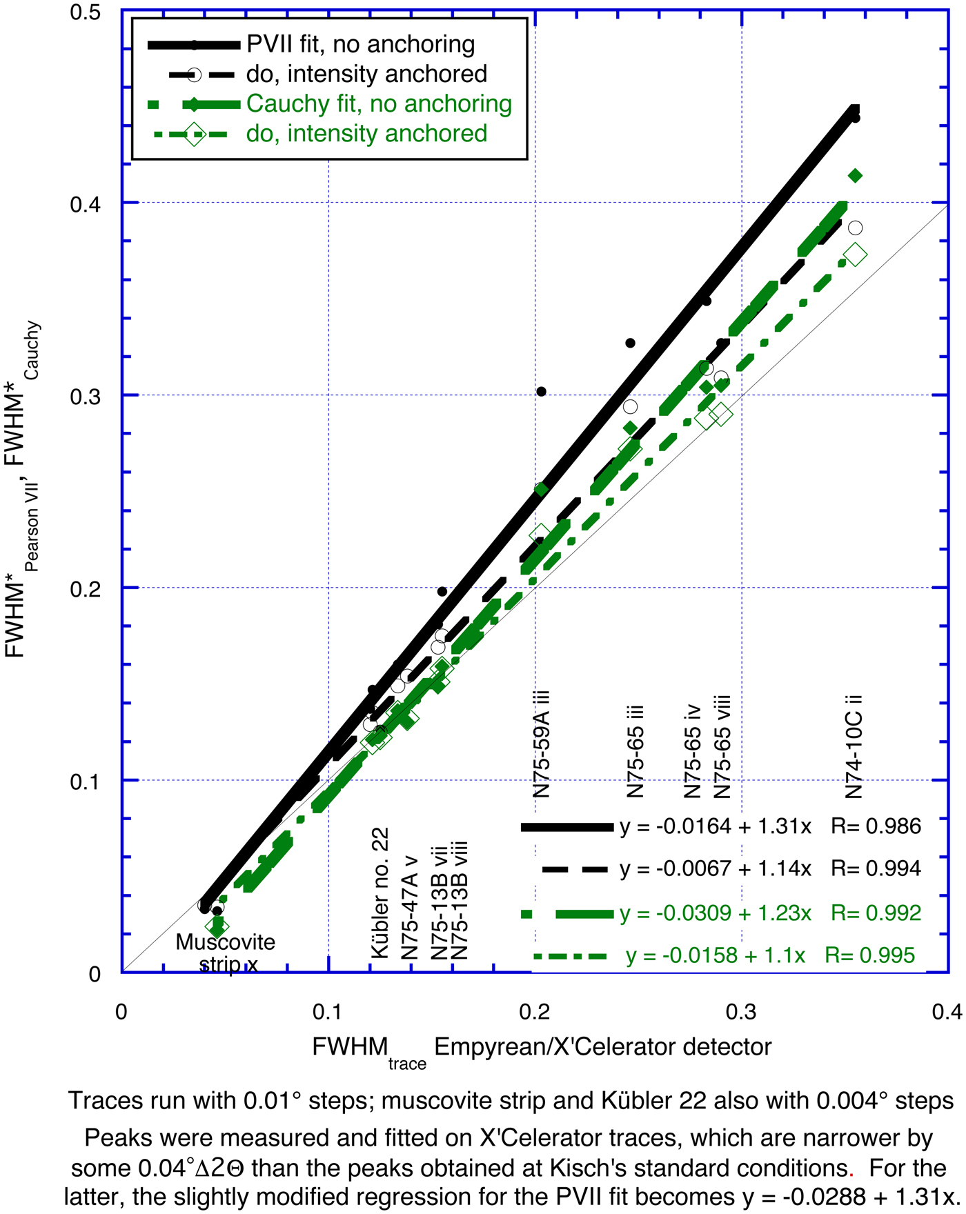
Fig. 5. FWHM*PVII vs. FWHMtrace for six polished-slate standards and one muscovite strip standard, measured by an Empyrean/X'Celerator detector, 0.1° steps (except where otherwise indicated). Also indicated is FWHM*PVII with fit intensity anchored at the trace-peak maximum.
These differences increase strongly with the value of FWHMtrace. In addition, they are related to the peak shape, notably the extent of the tails, and the consequent reduction in intensity: they are greatest for standards N75-59A (Fig. 3) and N74-10C, which have very broad tails, small for N75-47A and N75-13B, which have narrow tails, and almost nil for the muscovite strip (Fig. 4), which has very narrow tails. As the extent of this broadening is variable, FWHM*PVII cannot be converted to FWHMtrace without reference to the original trace.
In order to evaluate the contribution of reduced peak intensity on the peak broadening upon fitting of the polished slates, we have also fitted them by anchoring their peak intensity to that of the unfitted traces (see Fig. 5). The reduction of FWHM* upon peak-intensity anchoring is about half of the Pearson VII fit for the Cauchy fit, reflecting the much smaller reduction of its peak intensity; the change in peak area and the reduction of reliability are minor. In most, both ΔFWHM*PVII (= ΔFWHM*PVII – FWHMtrace) and ΔFWHM*Cauchy (= ΔFWHM*Cauchy – FWHMtrace) are reduced by about half with respect to that without intensity anchoring. FWHM*Cauchy with anchored intensity (FWHM☨Cauchy) is very close to FWHMtrace, with ΔFWHM☨Cauchy being ≤0.025°Δ2θ, ≤10% of FWHMtrace (except for the muscovite strip).
The authors therefore might recommend the intensity-anchoring method, were it not for the fact that in decomposing composite reflections the expected intensities of each constituent are unknown, though in most cases they can be calculated from those of higher-order reflections.
Fitted FWHM* on PSS from various laboratories
We have also compared the divergences of the FWHM* values obtained by various laboratories on the PSS from those measured on the profiles by Kisch at his standard conditions (Fig. 6).
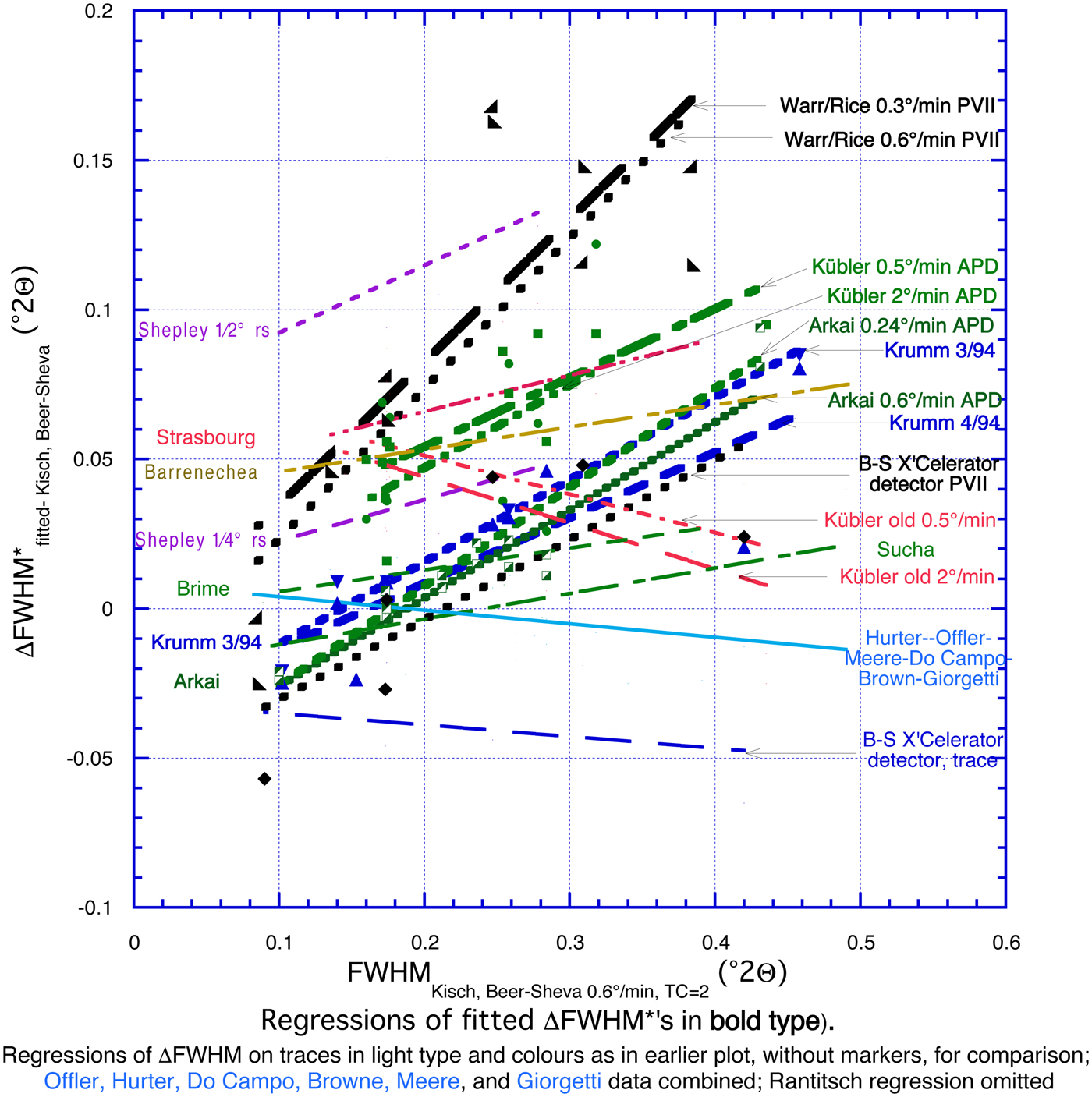
Fig. 6. ΔFWHM*, the difference between the fitted FWHM* values obtained by nine laboratorieσ ν Kisch's polished-slate standards and muscovite strips and FWHMtrace measured on the trace profiles by Kisch at his standard conditions. Regressions for fitted values in bold type: Pearson VII fits in black; APD-10 fits in green; and Pearson V fits in blue. The low-intensity trace of standard N74-10C iv on Kübler APD-10, 2°/min, has been omitted. Regressions for ΔΦΩHM on traces in light type (from Fig. 1) are provided for comparison. Contributors and their laboratories are listed in the acknowledgments. Regressions are as follows : Warr & Rice 0.6°/min y = –0.0271 + 0.504x, R = 0.8; Warr & Rice 0.3°/min y = –0.0132 + 0.479x, R = 0.844; Kübler 0.5°/min y = 0.00791 + 0.231x, R = 0.778; Kübler 2°/min y = –0.0082 + 0.277x, R = 0.524; Árkai 0.24°/min y = –0.0586 + 0.331x, R = 0.967; Árkai 0.6°/min y = –0.0552 + 0.294x, R = 0.959; Krumm 4/94 y = –0.0353 + 0.219x, R = 0.828; Krumm 3/94 y = –0.0393 + 0.275x, R = 0.984; X'Celerator detector Beer-Sheva y = –0.057 + 0.267x, R = 0.753.
The regressions for ΔFWHM are appreciably steeper than those for FWHMtrace of the unfitted values (Fig. 5). In fact, they are steepest (equation +0.48–0.50 × FWHMtrace) for the ‘FWHM*’ values fitted with the Pearson VII function by Warr and Rice (Reference Warr and Rice1994) because these appear to be IBs of the Pearson VII function, being broader by 22% than the FWHMPVII breadths, which would be +0.21–0.23 × FWHMtrace. They are somewhat less steep (+0.22–0.33 × FWHMtrace) for those fitted with APD-10 parabolic functions (Arkai, Kübler) and with the Pearson V function close to the Cauchy function (Krumm) (i.e. ΔFWHM* tends towards fixed percentages of FWHMKisch). This strong increase of ΔFWHM* with FWHMtrace contrasts markedly with the more uniform peak broadening of the unfitted peaks due to high TC/W t ratios.
Figure 7 shows logarithmic equations for ΔFWHM* vs. FWHMtrace (bold regressions). Their correlation coefficients, R (not given), are much greater than of the linear equations for the Pearson VII fits: R = 0.88 and 0.91 for Warr and Rice; R = 0.85 for the X'Celerator detector, Beer-Sheva – in part due to the narrow FWHM* of the muscovite strip. They are only insignificantly better (R = 0.86 and 0.98 vs. 0.83 and 0.98) for the Pearson V fits (Krumm – muscovite strip fitted with the Gauss function) and almost identical for the APD-10 fits by Árkai (R = 0.96 and 0.97 in both cases). They are similar to the APD-10 fits by Kübler, but very poor in both cases (R = 0.81 and 0.5 vs. 0.78 and 0.52).
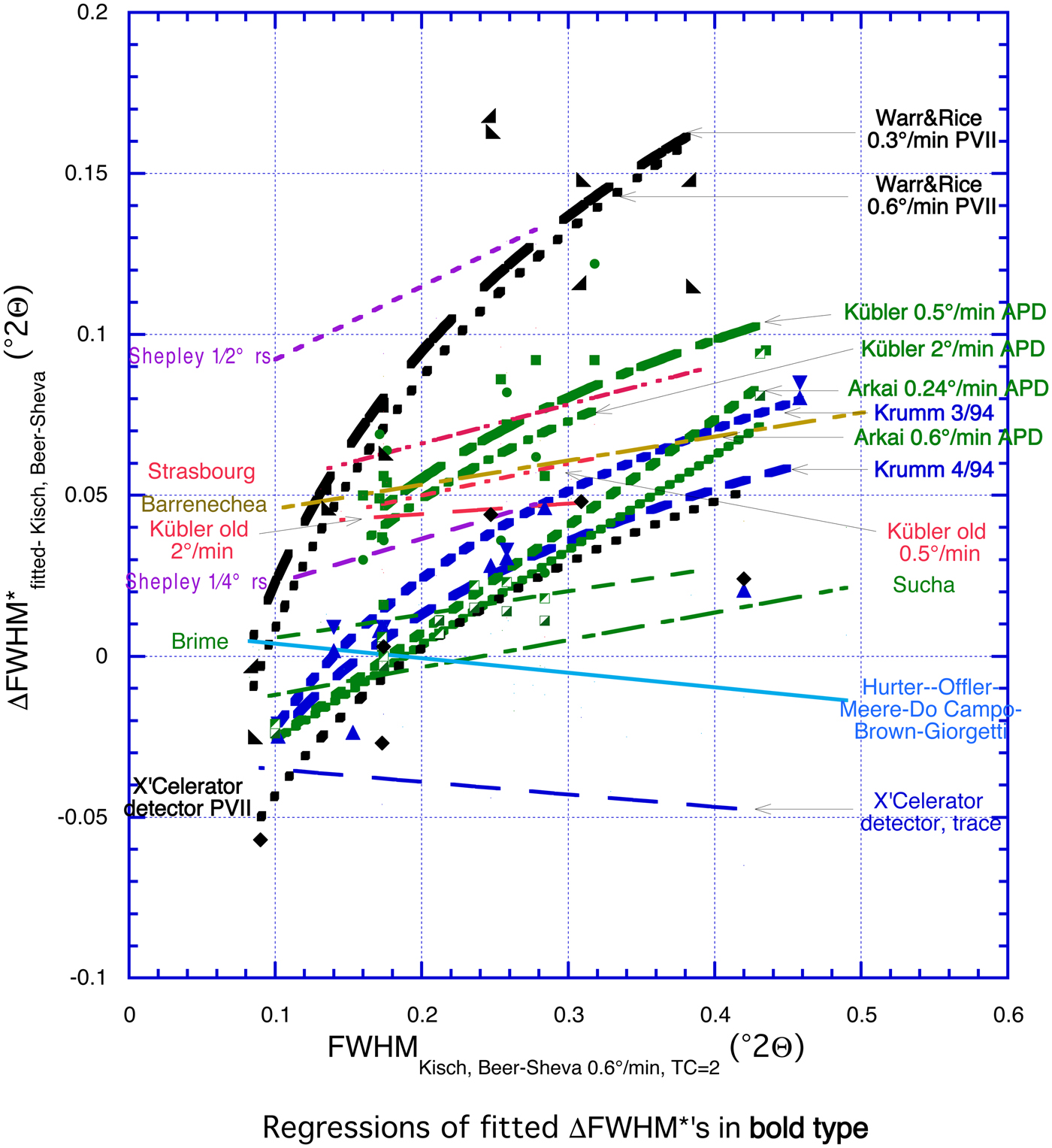
Fig. 7. ΔFWΗM*fitted of the fitted values vs. FWHMtrace (bold regressions) with logarithmic equations.
FWHM* as fitted with the Cauchy and Pearson VII functions
Figure 8 shows FWHM* values fitted with the Cauchy and Pearson VII functions for 33 pipetted slides with negligible I-S mixed layers and the polished-slate standard. For the pipetted slides, FWHM*PVII and FWHM*Cauchy are broader by 15% and 7% on average, respectively, than FWHMtrace, with regressions showing very high correlation coefficients (99.2% and 99.5%, respectively). The slightly steeper regression slopes and lower reliabilities for the polished-slate and muscovite-strip standards are due to the narrow FWHMtrace values for the polished slate N75-59A and, to a somewhat lesser extent, due to the polished slates N75-65 and N74-10C (see below). If the FWHM*PVII (X'Celerator) vs. FWHMtrace regression for the polished slates, FWHM*PVII (X'Celerator) = 1.22 × FWHM*PVII – 0.010° is modified by adding the average 0.04°Δ2θ difference between FWHMstandard conditions and FWHMX'Celerator, which becomes FWHM*PVII (standard conditions) = 1.22 × FWHM*PVII + 0.030°. These differences are highlighted on a plot of the incremental peak broadening ΔFWHM*PVII–trace/FWHMtrace (FWHM*PVII/FWHMtrace – 1) and ΔFWHM*Cauchy–trace/FWHMtrace (FWHM*Cauchy/FWHMtrace – 1) vs. FWHMtrace (Fig. 9).
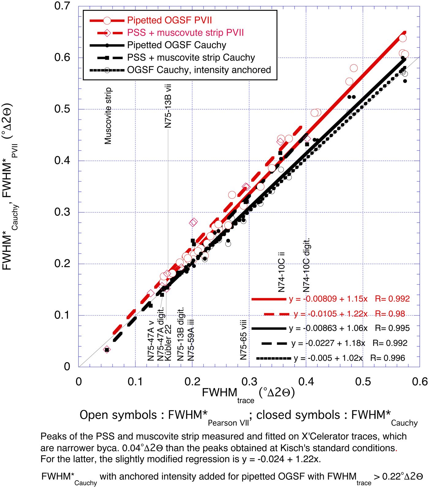
Fig. 8. FWHM* as fitted with the Cauchy and Pearson VII functions for 33 pipetted, oriented grain-size fractions (OGSF) and six polished-shale/slate standards (PSS) and one muscovite strip plotted against FWHMtrace (standard conditions).
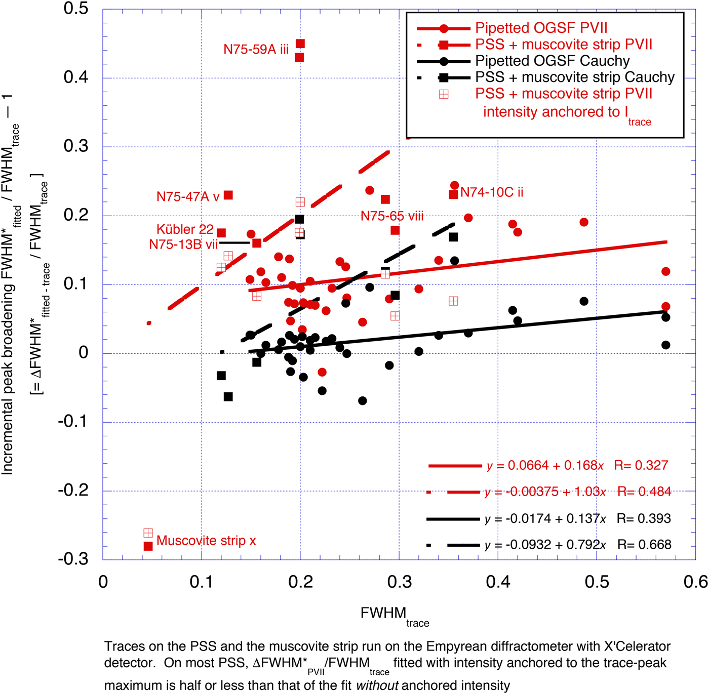
Fig. 9. Incremental peak broadening ΔFWΗM*PVII–trace/FWHMtrace [FWHM*PVII/FWHMtrace–1] and ΔFWHM*Cauchy–trace/FWHMtrace [FWHM*Cauchy/FWHMtrace–1] for the samples in Fig. 8 plotted against FWHMtrace. FWHM*Cauchy with anchored intensity given for the pipetted, oriented grain-size fractions (OGSF) with FWHMtrace > 0.22°Δ > 0.
The incremental peak broadening ΔFWHMPVII – trace/FWHMtrace is 3–20% of FWHMtrace (average 12%; one exception with a broad peak top). Both this broadening and the reduction of the peak maxima I*PVII/Itrace are closely related to the fitting reliability R, with the percentage broadening ΔFWHM*PVII/FWHMtrace increasing from 3 to 8% for the best R ≥97%, through 7–14% for intermediate R ≥95–97% and 13–20% for the poorest fit R <95%, whereas I*PVII/Itrace approaches the reciprocal of FWHM*PVII/FWHMtrace.
The ΔFWHM*Cauchy–trace/FWHMtrace is much smaller than ΔFWHM*PVII–trace/FWHMtrace: for the pipetted slides, it ranges from –8 to + 10% (average 3%). The reliabilities R of the Cauchy function fits (95.7–98.9%) are almost invariably greater than those of the Pearson VII function (92.9–97.4%) by 1–5%; the FWHM*Cauchy values are narrower by 0.01–0.07°Δ2θ or 5–17% than FWHM*PVII. Although FWHM*Cauchy still differs slightly from the FWHM values on the diffraction traces, predominantly being slightly broader, they are much closer compared to their FWHM*PVII counterparts, usually within 0.02°Δ2θ. This markedly lesser broadening of FWHM* of the Cauchy relative to the Pearson VII function is the result of its stronger top curvature and notably faster tail fading (less ‘smoothing’).
The Voigt and the closely approximate pseudo-Voigt functions are intermediate between the Cauchy (Lorentz) and Gauss functions. As FWHMGauss and, to a lesser extent, FWHMCauchy are, on average, both broader than FWHMtrace, the FWHM on the Voigt and pseudo-Voigt functions will consequently also be broader, and we have therefore plotted FWHM for these functions.
The notably steeper slopes of both the ΔFWHM*PVII–trace/FWHMtrace and ΔFWHM*Cauchy–trace/FWHMtrace vs FWHMtrace regressions for the PSS for those of the pipetted slides are due to the broad ΔFWHM*PVII–trace and ΔFWHM*Cauchy–trace of the broader polished-slate standards N75-59A (cf. Figs 3b,c, 5) and, to a lesser extent, N75-65 and N74-10C than for pipetted slides with similar FWHMtrace. Their fitting reliabilities RPVII = 90.2–95.4% and RCauchy = 94.4–97.6% are only slightly lower than for most pipetted slides.
In contrast, for the muscovite strip, both ΔFWHM*PVII–trace and ΔFWHM*Cauchy–trace are markedly negative, with very poor reliabilities of RPVII = 84% and RCauchy = 86%, due to the virtual absence of tails: in this case, the Gaussian function produces the best fit (Fig. 6).
Thus, the FWHM*Cauchy of pipetted slides, although still not very good, approximates much closer that measured on the XRD traces than FWHM*PVII, and the FWHM☨Cauchy with anchored intensity is virtually identical to FWHMtrace.
Fitted functions for low-angle peaks other than muscovite/illite 10 Å
The peak-broadening effects are similar for other low-angle peaks with wide tails, such as chlorite 14 Å, but decrease with narrowing and lowering of the peak tails at higher 2θ angle reflections.
For the chlorite 7 Å peak, FWHM*PVII remains broader than FWHMtrace by up to 0.03°Δ2θ – approximately half that for muscovite/illite 10 Å – whereas for FWHM*Cauchy, the broadening/narrowing effects are partly inverted: it is between 0.03°Δ2θ narrower to 0.02°Δ2θ broader than FWHMtrace.
Compared with the fitting reliabilities of the illite/muscovite 10 Å peaks, those of the Pearson VII and Cauchy functions converge somewhat: those of the Pearson VII function are slightly ‘higher’ (R = 94.5–97.8% and 92.7–97.0%. respectively) and those of the Cauchy function are slightly ‘lower’ (R = 95.4–98.3% and 95.7–98.9%, respectively), but RCauchy remains higher than RPVII by –0.4% to 3.5%. FWHM*Cauchy values are still narrower by –0.01°Δ2θ to 0.05°Δ2θ than FWHM*PVII. Although they still differ somewhat from the FWHM values on the diffraction traces, predominantly still being slightly broader, they are much closer, usually within 0.02°Δ2θ. Similar to the previous peaks, this lesser broadening of FWHM* of the Cauchy relative to the Pearson VII function is the result of its stronger top curvature and notably faster tail fading (less ‘smoothing’).
In terms of muscovite/illite 5 Å, both Pearson VII and Cauchy show good fits (R usually >95%); FWHM*PVII is within ±0.015°Δ2θ of that of the trace, whereas FWHM*Cauchy is commonly narrower by 0.005–0.030°Δ2θ, even when its RCauchy is slightly higher than RPVII.
From the 10 Å through the 7 Å to the 5 Å peaks, the ΔFWHM* values thus tend to narrow to close to FWHMtrace: from largely much broader to close to that for the Pearson VII fits, and from mostly slightly broader to predominantly somewhat narrower than FWHMtrace.
For higher-angle mica peaks, FWHM*PVII and FWHM*Cauchy converge, usually differing only by 0.01–0.03°Δ2θ for the 5 Å peak and even less for the 3.3 Å peak; for the quartz 4.255 Å/20.86°2θ peak, FWHM*PVII tends to be narrower by up to 0.005°Δ2θ than FWHM*Cauchy; both are within 0.01°Δ2θ of FWHMtrace. For these peaks, the Voigt or pseudo-Voigt functions may give FWHM breadths that are intermediate between FWHM*PVII and FWHM*Cauchy, and thus somewhat closer to FWHMtrace. However, as that is not the subject of this contribution, it will not be considered further.
DISCUSSION
The shape of the traces of the broader polished-slate standard peaks, with sharper peak tops and longer tails, compared to the pipetted slides, has been referred to as ‘super-Lorentzian’ (or ‘super-Cauchy’), which differs from the Lorentzian shape in its grain-size range. The “Lorentzian shape is the case where ~70% of the whole crystallites have a size within the range from half to twice of the median size” (Hosokawa et al., Reference Hosokawa, Naito, Nogi and Yokoyama2012, p. 272); it “is predicted for broader distribution of the crystallite size” (Himeda, Reference Himeda2012, p. 11). The admixture of coarse clastic mica accounts for the broad grain-size range in the polished slates compared with the pipetted slides.
The FWHM*PVII of the Pearson VII function fitted to the muscovite/illite 10 Å peaks is almost consistently broader than FWHMtrace of the diffraction profile. Moreover, the extent of this broadening is not uniform, but depends on the peak shape, being larger for peaks with broader tails (notably the polished slates). Due to this variability, it cannot be converted into FWHMtrace without reference to the original trace. The Pearson VII function is therefore ‘inappropriate’ for fitting FWHM of these peaks.
This broadening of FWHM* accounts largely for the high FWHM* values in the inter-laboratory calibration curve of Warr & Rice (Reference Warr and Rice1994, fig. 2) and the resulting inordinately broad anchizone limits of these authors and of Warr & Ferreiro-Mählmann (Reference Warr and Ferreiro Mählmann2015). The calibration of Warr & Rice (Reference Warr and Rice1994) using Pearson VII fittings of polished-slate standards against FWHMtrace by the present author gave inordinate broadening of IC*Warr & Rice = 1.512 × FWHMKisch – 0.0293° (Warr & Rice, Reference Warr and Rice1994, fig. 2) or ~1.512 × FWHMKübler – 0.090°, with a rather poor correlation coefficient of R2 = 0.945 (a logarithmic regression shows a much better correlation coefficient of R = 0.991); the corresponding anchizone limits of 0.29°Δ2θ and 0.54°Δ2Θ are much broader than Kisch’s 0.21°Δ2Θ and 0.375°Δ2θ and Kübler’s 0.25°Δ2θ and 0.42°Δ2Θ. This calibration was criticized by Kisch et al. (Reference Kisch, Árkai and Brime2004), who called for publication of the ‘raw’ uncalibrated data from Warr & Rice (Reference Warr and Rice1994) (i.e. FWHM as measured on their trace profiles). Ferreiro-Mählmann & Frey (Reference Ferreiro-Mählmann and Frey2012) also noted that “Kübler-index values obtained by the so-called CIS calibration are not compatible with Kübler–Frey–Kisch (Árkai, Aprahamian, Brime, Ferreiro-Mählmann, H. Krumm, Leoni, Petschick) calibrated Kübler indices.” The scatter of the points about their regression reflects the very different broadening percentage for the samples used.
RECOMMENDATIONS
The Pearson VII function should not be used to model FWHM of mica/illite 10 Å peaks; if peak fitting is unavoidable, use of the Cauchy function is preferable, particularly with peak-top intensity anchoring.
In the absence of a more appropriate function for fitting the slender-top and broad-tail ‘super-Lorentzian’ mica/illite 10 Å peaks, we strongly recommend that their FWHM only be measured directly on the diffraction trace, rather than on fitted functions. When the use of fitting functions is unavoidable (e.g. for resolution of the 10 Å peak from unresolved nearby peaks such as paragonite 9.66 Å or pyrophyllite 9.2 Å), we recommend the use of the fitting function that gives the best fit so far (i.e. Cauchy rather than Pearson VII [and Gauss for muscovite flakes]), and clearly indicate this.
ACKNOWLEDGMENTS
Of the scores of researchers who measured the author's sets of polished-slate standards and muscovite strips, the following kindly sent the results of their measurements and allowed their use: Péter Árkai, Budapest (5/1998); José Fernández Barrenechea, Madrid (1/1993); Covadonga Brime, Oviedo (7/1989); Patrick R.L. Browne and Solomon Woldemichael, Auckland (5/1994); Margarita Do Campo, Buenos Aires (3/1994); Gilbert Dunoyer de Segonzac, Ph. Larque, Strasbourg (6/1986); Martin Frey, Basel (11/1996); Giovanna Giorgetti and Isabella Memmi, Siena (6/1995); Suzanne Hurter, Ann Arbor, Michigan (2/1991); Stefan Krumm, Erlangen (3/1994); Bernard Kübler, Neuchâtel (4/1986); Patrick A. Meere, VU Amsterdam (4/1991); Robin Offler, Newcastle, NSW (1992); Gerd Rantitsch, Leoben (10/1995); Martin G. Shepley, Oxford (3/1991); Vlado Šuchá, Bratislava (2/1995); and Laurence N. Warr, Heidelberg (5/1992).
The author profited from discussions with Laurence Warr, Rafael Ferreiro-Mählmann and Jan Środoń. The manuscript was much improved by meticulous reviews by Ömer Bozkaya and two anonymous reviewers.


