


NOMENCLATURE
- A
-
Jacobian matrix
- I
-
identity matrix
- L g
-
gust length
- r k
-
relative information content
- R
-
residual vector
- S
-
snapshot matrix
- v g
-
gust excitation vector
- w
-
state-space vector
- z
-
reduced-order model basis vector
Greek Symbol
- λ
-
POD eigenvalue
- ν
-
POD eigenvector
- φ
-
POD mode vector
- Φ
-
POD mode matrix
- ω
-
reduced frequency
1.0 INTRODUCTION
Dynamic responses to atmospheric turbulence describe several critical load cases during the aircraft design process, demanding highly accurate results at low cost to investigate a large range of parameters. Current industrial practice is based on linear aerodynamics in frequency domain, mostly the doublet lattice method(Reference Albano and Rodden1). Thus, examples for this are widespread from isolated wings(Reference Giesing, Rodden and Stahl2) to full aircraft configurations(Reference Kier3). While these methods are computationally highly efficient, they cannot capture transonic, viscous or thickness effects. To improve the accuracy of the predicted loads, correction factors are applied based on either experimental or Computational Fluid Dynamics (CFD) data(Reference Dimitrov and Thormann4). However, these corrections are often introduced only at zero frequency, and thus deviations at higher frequencies, important for shorter gust lengths, cannot be captured accurately.
Despite the overwhelming computational cost, CFD methods alone have been used to investigate gust encounter in the past few years, offering accurate results also at non-linear conditions. Results are available for a large range of problems from aerofoils to civil aircraft(Reference Raveh5,Reference Reimer, Ritter, Heinrich and Krüger6) . An improvement in efficiency, while maintaining the fidelity of the underlying non-linear CFD model, can be achieved by applying linearised frequency-domain methods. The governing equations are linearised around a non-linear steady-state solution assuming small amplitude harmonic motion. Results are widespread from turbomachinery to fixed-wing aircraft, including aerofoils and complete airframes, reporting consistently significant cost-saving factors, independent of the problem size(Reference Clark and Hall7-Reference Thormann and Widhalm9). An extension towards gust response simulations has also been published(Reference Bekemeyer, Thormann and Timme10).
Reduced-order modelling is considered a promising approach to further reduce computational cost, while still preserving accuracy of the underlying full-order model(Reference Lucia, Beran and Silva11). A common model reduction technique is based on Proper Orthogonal Decomposition (POD)(Reference Taira, Brunton, Dawson, Rowley, Colonius, McKeon, Schmidt, Gordeyev, Theofilis and Ukeiley12), first used, in the context of fluid dynamics, to model coherent structures in turbulent flow fields(Reference Lumley13). A small eigenvalue problem, related to snapshots generated by analysing the full system either numerically or experimentally, is solved to obtain POD modes. This approach was soon extended towards frequency-domain sampling data to investigate a rather simple 12-degrees-of-freedom mass-spring-damper system combined with an incompressible three-dimensional vortex lattice method(Reference Kim14). Linearised CFD aerodynamics were first considered to analyse the dynamic response of a pitch-plunge aerofoil(Reference Hall, Thomas and Dowell15). Recently, an application for gust responses has been presented for a NACA0012 aerofoil in sub- and transonic flow conditions(Reference Bekemeyer and Timme16,Reference Thormann, Bekemeyer and Timme17) , showing excellent agreement at several orders of magnitude reduced computational cost. Combining POD with a linearised frequency-domain method not only reduces computational cost further, but, more importantly, an interpolation for frequencies not pre-computed can be avoided. Further, a model is obtained that can easily be extended for structural degrees-of-freedom(Reference Bekemeyer and Timme16,Reference Bekemeyer and Timme18) .
This paper presents a reduced-order modelling approach for a three-dimensional, industry relevant test case. The full-order system behaviour is sampled by computing complex-valued gust responses at several discrete frequencies. Using the standard snapshot POD technique, a small eigenvalue problem, correlated to the sampling data, is solved and the number of considered modes is truncated by applying an energy criterion. These modes are discussed to analyse the main region of interest for dynamic gust responses. Once the modal basis is available, the linearised Reynolds-Averaged Navier-Stokes (RANS) equations are projected onto the POD subspace and rapidly solved for an arbitrary number of frequencies to analyse 1-cos gust responses. Besides lift coefficient also surface pressure distribution are compared for results given by the reduced-order model and full-order, unsteady time-marching simulations. Using high-fidelity aerodynamics directly offers an increased confidence in the predicted loads. While the industrial correction approach requires expert knowledge, this can be omitted in a purely CFD-based approach. Thus, loads calculation becomes more streamlined reducing time and cost per design iteration. Even though CFD knowledge is needed during the model generation, the resulting system can be applied to analyse the aircraft response without in-depth CFD experience. This enables the use of accurate loads in the aircraft design and certification process.
2.0 NUMERICAL METHOD
The governing equation in semi-discrete vector form is
 $$\begin{equation}
\dot{{\bf w}}={\bf R}({\bf w}, {\bf v}_{\mathrm{g}}),
\end{equation}$$
$$\begin{equation}
\dot{{\bf w}}={\bf R}({\bf w}, {\bf v}_{\mathrm{g}}),
\end{equation}$$
where R is the non-linear residual corresponding to the fluid unknowns w, while v g denotes external disturbances due to gusts. The difference between an equilibrium solution w 0 and the state-space vector w is introduced as
 $$\begin{equation}
\Delta {\bf w}={\bf w}-{\bf w}_0,
\end{equation}$$
$$\begin{equation}
\Delta {\bf w}={\bf w}-{\bf w}_0,
\end{equation}$$
and accordingly for external disturbances. A first-order Taylor expansion is used to express the change in residual around the equilibrium point,
 $$\begin{equation}
\Delta \dot{{\bf w}}={\bf R}({\bf w}_0,{\bf v}_{\mathrm{g}0})+\frac{\partial {\bf R}}{\partial {\bf w}} \Delta {\bf w} + \frac{\partial {\bf R}}{\partial {\bf v}_{\mathrm{g}}} \Delta {\bf v}_{\mathrm{g}},
\end{equation}$$
$$\begin{equation}
\Delta \dot{{\bf w}}={\bf R}({\bf w}_0,{\bf v}_{\mathrm{g}0})+\frac{\partial {\bf R}}{\partial {\bf w}} \Delta {\bf w} + \frac{\partial {\bf R}}{\partial {\bf v}_{\mathrm{g}}} \Delta {\bf v}_{\mathrm{g}},
\end{equation}$$
where
 $\frac{\partial {\bf R}}{\partial {\bf w}}$
describes the Jacobian matrix A and R(w
0, v
g0) is by definition zero.
$\frac{\partial {\bf R}}{\partial {\bf w}}$
describes the Jacobian matrix A and R(w
0, v
g0) is by definition zero.
Assuming harmonic motions for the disturbance vector Δw and external excitation vector Δv g, the system is transferred into frequency domain. Thus, Equation (3) becomes
 $$\begin{equation}
\left( A - i\omega I \right) \hat{{\bf w}} = - \frac{\partial {\bf R}}{\partial {\bf v}_{\mathrm{g}}} \hat{{\bf v}}_{\mathrm{g}},
\end{equation}$$
$$\begin{equation}
\left( A - i\omega I \right) \hat{{\bf w}} = - \frac{\partial {\bf R}}{\partial {\bf v}_{\mathrm{g}}} \hat{{\bf v}}_{\mathrm{g}},
\end{equation}$$
with
 $\hat{ {\bf w}}$
and
$\hat{ {\bf w}}$
and
 $\hat{ {\bf v}}_{\mathrm{g}}$
denoting complex-valued Fourier coefficients. A first-discretise-then-linearise, matrix-forming approach with an analytical, hand-differentiated Jacobian matrix is used to obtain the linear system in Equation (4). Further details about the applied LFD implementation are available(Reference Thormann and Widhalm9). A finite-difference evaluation,
$\hat{ {\bf v}}_{\mathrm{g}}$
denoting complex-valued Fourier coefficients. A first-discretise-then-linearise, matrix-forming approach with an analytical, hand-differentiated Jacobian matrix is used to obtain the linear system in Equation (4). Further details about the applied LFD implementation are available(Reference Thormann and Widhalm9). A finite-difference evaluation,
 $$\begin{equation}
\frac{\partial {\bf R}}{\partial {\bf v}}_{\mathrm{g}} \hat{{\bf v}}_{\mathrm{g}}= \frac{{\bf R}({\bf w}_0, +\varepsilon \hat{{\bf v}}_{\mathrm{g}}) -{\bf R}({\bf w}_0, -\varepsilon \hat{{\bf v}}_{\mathrm{g}})}{2\varepsilon },
\end{equation}$$
$$\begin{equation}
\frac{\partial {\bf R}}{\partial {\bf v}}_{\mathrm{g}} \hat{{\bf v}}_{\mathrm{g}}= \frac{{\bf R}({\bf w}_0, +\varepsilon \hat{{\bf v}}_{\mathrm{g}}) -{\bf R}({\bf w}_0, -\varepsilon \hat{{\bf v}}_{\mathrm{g}})}{2\varepsilon },
\end{equation}$$
with a known gust shape vector
 $\hat{{\bf v}}_{\mathrm{g}}$
and ε as the finite-difference step size is used to evaluate the right-hand side term in Equation (4) without computing the matrix explicitly. The cost of two additional residual evaluations is required to construct the right-hand side before solving the linear system, while the computational overhead of forming and storing the matrix explicitly can be avoided.
$\hat{{\bf v}}_{\mathrm{g}}$
and ε as the finite-difference step size is used to evaluate the right-hand side term in Equation (4) without computing the matrix explicitly. The cost of two additional residual evaluations is required to construct the right-hand side before solving the linear system, while the computational overhead of forming and storing the matrix explicitly can be avoided.
Furthermore, an analytical description of the gust vector is introduced as
 $$\begin{equation}
\hat{{\bf v}}_{\mathrm{g}}({\bf x},\omega )=v_{gz} e^{i \bm{\varphi }({\bf x},\omega )},
\end{equation}$$
$$\begin{equation}
\hat{{\bf v}}_{\mathrm{g}}({\bf x},\omega )=v_{gz} e^{i \bm{\varphi }({\bf x},\omega )},
\end{equation}$$
where v gz and φ (x, ω) denote the constant vertical gust amplitude and the phase shift vector according to the spatial location vector x, respectively. The phase shift can either be obtained from a Fourier transform of a sinusoidal time-domain signal or, as known from linear potential theory(Reference Rodden19), using the expression
 $$\begin{equation}
\bm{\varphi }({\bf x},\omega )= \left({\bf x}+x_0 \right)\frac{\omega }{c_{\text{ref}}},
\end{equation}$$
$$\begin{equation}
\bm{\varphi }({\bf x},\omega )= \left({\bf x}+x_0 \right)\frac{\omega }{c_{\text{ref}}},
\end{equation}$$
where x 0 is the initial distance between gust and airframe. A more detailed discussion about the frequency-domain gust response method can be found elsewhere(Reference Bekemeyer, Thormann and Timme20).
2.1 Proper orthogonal decomposition
Excellent reviews on POD are published and offer a more in-depth, theoretical description of the method(Reference Holmes, Lumley, Berkooz and Rowley21,Reference Berkooz, Holmes and Lumley22) while here only a brief overview is provided. POD is a modal decomposition technique that extracts modes by optimising the mean square of the variables of interest(Reference Taira, Brunton, Dawson, Rowley, Colonius, McKeon, Schmidt, Gordeyev, Theofilis and Ukeiley12). A minimal number of modes results from decomposing an ensemble of data trying to capture a predefined amount of energy. Since the system size is too large for the classical POD method, the method of snapshots is applied instead(Reference Sirovich23). Thus, the full-order model is analysed at K discrete reduced frequencies by solving Equation (4), while adjusting the right-hand side term accordingly. The solution snapshots
 $\hat{{\bf w}}$
are stored as columns in the matrix S as
$\hat{{\bf w}}$
are stored as columns in the matrix S as
 $$\begin{equation}
S= \left[\hat{{\bf w}}^1 , \hat{{\bf w}}^2 ,\dots , \hat{{\bf w}}^{K} \right].
\end{equation}$$
$$\begin{equation}
S= \left[\hat{{\bf w}}^1 , \hat{{\bf w}}^2 ,\dots , \hat{{\bf w}}^{K} \right].
\end{equation}$$
The columns of the POD basis Φ are linear combinations of the columns of the snapshot matrix as
 $$\begin{equation}
{\bm\varphi} _k = S \bm{\nu }_k.
\end{equation}$$
$$\begin{equation}
{\bm\varphi} _k = S \bm{\nu }_k.
\end{equation}$$
Unit length of basis vectors φ k is ensured by scaling ν k . The best possible approximation in Equation (9) is then obtained by solving the corresponding eigenvalue problem of dimension K,
 $$\begin{equation}
S^H S \bm{\nu }_k = \lambda _k \bm{\nu }_k.
\end{equation}$$
$$\begin{equation}
S^H S \bm{\nu }_k = \lambda _k \bm{\nu }_k.
\end{equation}$$
Since S H S is positive definite and symmetric, all eigenvalues λ k are real and positive. The relative information content contributed to the system by a certain mode, also often referred to as energy, is given by
 $$\begin{equation}
r_k= \lambda _k \left(\sum _{i=0}^{K} \lambda _i \right)^{-1},
\end{equation}$$
$$\begin{equation}
r_k= \lambda _k \left(\sum _{i=0}^{K} \lambda _i \right)^{-1},
\end{equation}$$
and can be used to decrease the number of modes further by only considering those with a high relative information content.
The corresponding reduced-order model (ROM) is constructed by expressing the state-space vector
 $\hat{{\bf w}}$
as
$\hat{{\bf w}}$
as
 $$\begin{equation}
\hat{{\bf w}} = \Phi \hat{{\bf z}}.
\end{equation}$$
$$\begin{equation}
\hat{{\bf w}} = \Phi \hat{{\bf z}}.
\end{equation}$$
The small-sized reduced system is obtained through a Galerkin projection on Equation (4),
 $$\begin{equation}
\left( \Phi ^H A \Phi - i \omega I \right) \hat{{\bf z}} = - \Phi ^H \frac{\partial {\bf R}}{\partial {\bf v}_{\mathrm{g}}}\hat{{\bf v}}_{\mathrm{g}}.
\end{equation}$$
$$\begin{equation}
\left( \Phi ^H A \Phi - i \omega I \right) \hat{{\bf z}} = - \Phi ^H \frac{\partial {\bf R}}{\partial {\bf v}_{\mathrm{g}}}\hat{{\bf v}}_{\mathrm{g}}.
\end{equation}$$
Solving the ROM, represented by Equation (13), at an arbitrary number of frequencies and then reconstructing full-order solutions is an efficient way to investigate dynamic gust responses. Since an analytical derivation of the matrix
 $\frac{\partial {\bf R}}{\partial {\bf v}_{\mathrm{g}}}$
is currently under development, all right-hand sides for the ROM are sampled, projected and stored explicitly while forming the model.
$\frac{\partial {\bf R}}{\partial {\bf v}_{\mathrm{g}}}$
is currently under development, all right-hand sides for the ROM are sampled, projected and stored explicitly while forming the model.
2.2 Computational fluid dynamics method
Results are produced with the DLR-TAU code(Reference Schwamborn, Gerhold and Heinrich24) solving the RANS equations in conjunction with the Spalart-Allmaras turbulence model(Reference Spalart and Allmaras25). The field velocity approach which adds an artificial mesh velocity based on the defined excitation shape is used to include gusts(Reference Parameswaran and Baeder26). Inviscid fluxes are discretised by applying a central scheme with scalar artificial dissipation of Jameson, Schmidt and Turkel(Reference Jameson, Schmidt and Turkel27), while the Green-Gauss theorem is used to compute gradients, necessary for viscous and source terms. Steady-state solutions are obtained by utilising local time-stepping and the backward Euler method with lower-upper Symmetric-Gauss-Seidel iterations(Reference Dwight28). Convergence is further accelerated using a 2 v multigrid scheme.
All unsteady simulations are performed using dual time-stepping together with the second-order backward differentiation formula. Unsteady, time-dependent gust response simulations are produced with a time-step size of 0.00178 s and a fixed number of time steps of 1,024, based on previous numerical experiments. Linear systems are solved using a generalised conjugate residual solver with deflated restarting(Reference Xu, Timme and Badcock29). A block incomplete lower-upper factorisation of the Jacobian matrix with zero level of fill-in is applied for preconditioning(Reference Saad30). A total of 100 Krylov vectors, 20 of which are used for the deflated restarting process, are considered to solve the system. A drop of seven orders of magnitude in the density residual is used as convergence criterion. Since the reduced-order model is built assuming that the snapshots form a subspace of the eigenspace of the Jacobian matrix, the convergence criterion needs to be more stringent compared to a direct frequency-domain gust analysis(Reference Bekemeyer, Thormann and Timme20).
3.0 RESULTS
A large civil aircraft with a wingspan of approximately 60 m is investigated to demonstrate the maturity of the method for a test case of industrial interest. The mesh shown in Fig. 1(a) consists of nearly 8 million points, of which 130,000 are on the surface. Engine nacelles are simulated as flow-through. An elastic trimming procedure based on Broyden’s method(Reference Broyden31), balancing lift and weight while ensuring zero pitching moment, is used to obtain a steady-state solution at a representative freestream Mach number and altitude. In total, 94 structural modes are included and an artificial trimming mode representing the elevator deflection is applied. During the trimming process, the elevator deflection and the angle-of-attack are iteratively adjusted until the desired coefficients are reached. Within each iteration step the mesh is deformed according. Finally, the magnitude of the density residual is driven to converge seven orders of magnitude. The steady surface pressure distribution, shown in Fig. 1(b), contains a strong shock along the wingspan at roughly 70% chord length. A decrease of sectional lift towards the wing tip is caused by wing bending together with torsion. Since the elevator is deflected during the trimming process, a strong suction area around the leading edge is observed while no shock formation is present.
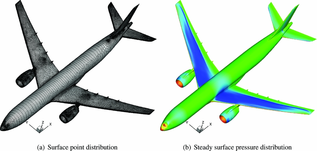
Figure 1. Surface mesh and steady-state surface pressure coefficient for civil aircraft.
The system response is sampled at 15 uniformly spaced reduced frequencies between 0 and 2. Different sampling strategies, including an exponential distribution, have not been tested yet and might prove beneficial since for aerofoil responses an improvement was observed(Reference Bekemeyer and Timme16). Furthermore, the inclusion of the complex conjugate of the snapshots while forming the reduced-order basis is not necessary since positive frequencies are sufficient to capture the system behaviour. The relative information content of all possible 15 POD modes is displayed in Fig. 2(a). With approximately 75%, the first mode contains most energy while the information content of all other modes decays nearly exponentially. The final mode has an energy content which is approximately six orders of magnitude below the first mode.
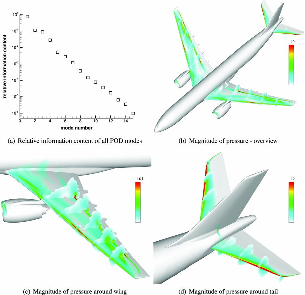
Figure 2. Relative information content of all POD modes and magnitude of pressure for first POD mode.
The pressure field for the first POD mode is shown for the whole aircraft, around the main wing and around the tail in Figs 2(b)–2(d), respectively. Several slices are displayed to visualise the three-dimensional structure of the POD mode also inside the flow field. The affected areas of the first POD mode are mainly the wing and the elevator, while no pressure fluctuations are present along the fuselage. On the upper wing surface, the governing flow features, namely the shock formation and the suction area around the leading edge, are clearly visible and describe the area of highest variations. Inside the field high values are concentrated close to the surface, and in particular around the shock formation and the suction area, while farther away from the surface the flow field is unaffected. Comparing inboard and outboard sections of the wing, it is found that the POD mode contains dominant features in the outboard region supporting the fact that gust loads define the outer wing structure. With no shock formation present on the tail, the elevator exhibits pressure deviations only around the suction line at the leading edge.
The influence of energy retained inside the ROM is investigated using a 1-cos gust with gust length L g = 116 m and an amplitude of 0.001% of the freestream velocity to ensure a dynamically linear response of the full-order time-marching solution. Since the reduced linear system is small, the spacing and number of considered frequencies for solving Equation (13) is of minor concern. However, it should be ensured that only frequencies inside the sampling range are used since extrapolation causes a significant reduction in accuracy for POD-based models. Time histories of the lift coefficient for the full-order reference solution and three reduced-order models, which only differ in the considered relative information content, are presented in Fig. 3(a). If 99.999% of the relative information content is included, resulting in 12 of 15 possible modes, the time-domain signal is rebuilt accurately. When the energy is decreased to 99.99%, reducing the number of modes to 7, also the peak value decreases while the overall shape, including the lift decay, is preserved. Since low-energy modes, which mainly contain high-frequency information, are omitted by reducing the number of modes inside the ROM, only local behaviour is affected, causing the maximum value to be underpredicted. Finally, with 99% energy, the overall tendency is still correct, but besides the peak value also the lift decay is no longer represented. Furthermore, results start to deviate from the steady solution since only four modes are retained which are mainly including low-frequency trends. In contrast to before, the peak value of lift is now predicted slightly higher compared to the reference solution. However, all three ROMs are very small in size compared to the initial full model, and the accuracy is generally very satisfying, requiring a zoom to see differences in peak lift values.
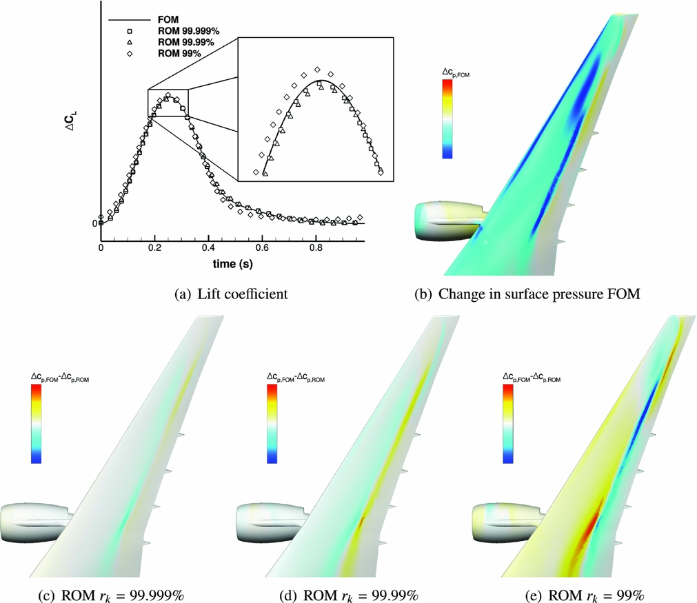
Figure 3. Investigation of modes retained in POD ROM using a 1-cos gust with L g = 116 m for time history of lift coefficient and change in surface pressure at ΔC L, max .
Surface pressure distributions on the starboard wing are compared between the full-order model (FOM) reference solution Fig. 3(b) and the three different ROMs, shown in Figs 3(c)–3(e). With decreasing mode number, the surface pressure around the shock position becomes more indistinct, while slight deviations are visible throughout the wing. In addition, if 99% of the energy is considered, differences are clearly visible close to the wing tip, resulting in an additional outer wing shock, which is not present in the FOM solution. Since the smallest ROM with only four modes overpredicts the maximum lift value, while both others slightly underpredict, the pressure deviations in Fig. 3(e) are reversed compared to Figs 3(c) and 3(d). For all remaining results, 12 modes are retained to identify occurring loads as accurately as possible. Thus, a huge reduction is achieved compared to the nearly 50 million degrees of freedom of the full system. Moreover, an even stronger reduction in size is possible when sacrificing accuracy.
Computational cost for building the reduced-order model, as well as for solving it, is displayed in Table 1. Since both the ROM and the unsteady time-marching approach require a steady-state solution, computational cost of the elastic trimming process is excluded. All values are non-dimensionalised by the computational cost of a full-order, time-domain reference solution. The most expensive part during the ROM generation is the frequency-domain sampling process with 0.345. However, sampling all snapshots in frequency domain already offers a cost-saving factor of about 3 compared to one full-order, unsteady time-marching solution. While the current model also needs to evaluate right-hand sides during the model construction, such cost, even though low at 0.025, can be avoided when an analytical description of the right-hand side matrix in Equation (13) is available, causing the efficiency of the generation process to increase further. Obtaining a 1-cos response using the ROM is approximately six orders of magnitude faster than solving the full-order model, while global coefficients, such as lift and pitching moment, are available at essentially no additional cost. Moreover, reconstructing surface pressure distributions is computationally as expensive as solving the reduced model. Shear forces and moments, essential during the aircraft design process, are produced together with the pressure distributions and thus come at no additional computational cost. It should be noted that the obtained time savings as well as the ROM accuracy is directly related to the number of samples generated. This sampling process strongly depends on the gust shapes and lengths of interest. However, also current industrial DLM-based methods sample the gust response behaviour in frequency domain. Thus, established industrial best practice can be directly applied during the POD model generation.
Table 1 Comparison of computational cost
Once the reduced-order model is available, several 1-cos gusts can be analysed at negligible computational cost. Dynamic responses for the coefficient of lift for three different representative gust lengths, namely L g = 58 m, 116 m and 174 m, are visualised in Fig. 4(a). Excellent agreement between the reduced model and the full-order reference solutions is obtained for all gust lengths. Only minor differences occur around maximum lift as already discussed above. When looking at the pitching moment coefficient in Fig. 4(b), again, good agreement is found. However, besides the slight deviations around the peak values minor oscillations arise during the moment decay for the shortest gust length. Creating sampling data at higher frequencies by applying an exponential instead of a uniform snapshot distribution might increase the accuracy of the ROM also for shorter gust lengths.
Figure 4. Time histories of lift and pitching moment coefficient for 1-cos gusts with L g = 58 m, 116 m and 174 m.
Finally, the ROM is used to investigate a dynamic response to a realistic 1-cos gust as defined by the European Aviation Safety Agency in CS 25.341(32). The gust length is chosen as L g = 116 m and the amplitude is nearly 7% of the freestream velocity. The change in lift coefficient over time is shown in Fig. 5(a). While for the overall shape good agreement is observed, minor differences in the maximum lift value as well as in the lift decay are visible. These discrepancies are caused by a dynamically non-linear response near the maximum lift coefficient during the time-marching simulation. The ROM, however, is constructed by a time-linearised RANS method and thus assumes a dynamically linear response, resulting in a slight overprediction of the maximum lift coefficient. Nevertheless, the ROM conservatively predicts loads at various orders of magnitude reduced computational cost. The absolute surface pressure difference at maximum lift coefficient is displayed in Fig. 5(b) to estimate the discrepancies when comparing both simulation techniques further. Since a non-linear shock motion and a non-linear amplitude decrease occur during the time-domain analysis, the highest error arises around the shock location. In addition, some minor discrepancies are present around the leading edge, caused by the same amplitude mechanism.
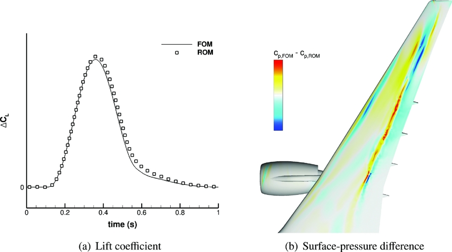
Figure 5. Time history of lift coefficient and surface-pressure difference at peak load for 1-cos gust with L g = 116 m.
4.0 CONCLUSIONS
This paper outlines a method to compute aerodynamic responses to gust encounter at several orders of magnitude reduced computational cost while preserving the accuracy of the underlying computational fluid dynamics solver. The governing Reynolds-averaged Navier-Stokes equations are linearised and transferred into frequency domain before projecting them on a small-sized modal basis. Proper orthogonal decomposition is applied for model reduction, based on sampling data generated at a few discrete frequencies using a linear frequency-domain solver. Following the projection, an arbitrary number of 1-cos gust responses can be obtained at negligible computational cost on a local desktop machine.
The presented test case is an elastically trimmed passenger aircraft at transonic flight conditions. The full-order model is sampled at 15 uniformly spaced reduced frequencies between 0 and 2 to construct a proper orthogonal decomposition-based reduced-order model. The relative information content of all possible modes is discussed and the first mode is analysed. Afterwards, a reduced-order model is created by retaining 12 modes, equivalent to 99.999% of the relative information content. Compared to the full-order model with nearly 50 million degrees of freedom a massive reduction in size is achieved. While accuracy is preserved when analysing various 1-cos gust responses using the applied strict energy criterion, reducing the retained relative information content could offer a more practical and applied solution since even stronger reductions are possible. Finally, the model is used to investigate a gust as defined by international certification regulations, showing good and conservative load predictions at several orders of magnitude reduced computational cost.
Gust loads analysis is an inherently multi-disciplinary process, and thus the inclusion of flight dynamics and structural dynamics is of general interest and required by regulation bodies. Therefore, a method combining the herein presented reduced-order model with traced eigenmodes of the Jacobian matrix has been proposed more recently(Reference Bekemeyer and Timme18,Reference Pagliuca, Bekemeyer, Thormann and Timme33) . Furthermore, an extension with a control system is straightforward, since small-sized matrices are produced from the reduced-order model, which are very similar to commonly applied models based on linear potential flow. This enables the use of accurate loads from computational fluid dynamics in a control system design e.g. for gust load alleviation.
ACKNOWLEDGEMENTS
The research leading to these results was co-funded by Innovate UK, the UK’s innovation agency, as part of the Enhanced Fidelity Transonic Wing project.


