


Introduction
Bromoform (CHBr3) is one of the volatile organic compounds (VOCs) originating with macroalgal and planktonic sources in the ocean, and bromoform is emitted from the ocean surface to the atmosphere (Quack & Wallace Reference Quack and Wallace2003). Bromoform is an important carrier of bromine to the troposphere, and its lifetime in the atmosphere is one to four weeks (Quack & Wallace Reference Quack and Wallace2003 and references therein). Although bromoform concentrations in the ocean have been measured widely, there is a lack of information regarding measurements of bromoform in the ice-covered seas. Sea ice may be a significant platform for the production of bromine compounds and a source for the atmosphere (Sturges et al. Reference Sturges, Cota and Buckley1992, Reference Sturges, Sullivan, Schnell, Heidt and Pollack1993, Reference Sturges, Cota and Buckley1997, Carpenter et al. Reference Carpenter, Wevill, Palmer and Michels2007). For example, polar ice algae is known to produce significant quantities of bromoform (Sturges et al. Reference Sturges, Cota and Buckley1992).
A surface slush layer (gap layer) is found extensively in Antarctic sea ice during the ice melting season (Haas et al. Reference Haas, Thomas and Bareiss2001, Kattner et al. Reference Kattner, Thomas, Haas, Kennedy and Dieckmannm2004, Ackley et al. Reference Ackley, Lewis, Fritsen and Xie2008, Zemmelink et al. Reference Zemmelink, Hintsa, Houghton, Dacey and Liss2008, Papadimitriou et al. Reference Papadimitriou, Thomas, Kennedy, Kuosa and Dieckmann2009). Snow accumulation over sea ice and the formation of superimposed ice leads to the formation of a slush layer below sea level (Haas et al. Reference Haas, Thomas and Bareiss2001). High biological activity has been found in this layer (Kattner et al. Reference Kattner, Thomas, Haas, Kennedy and Dieckmannm2004), suggesting that bromoform production could also be high in this layer. In addition, bromoform produced in the slush layer would accumulate because of limited gas diffusion through the snow and superimposed ice (Delille Reference Delille2006, Nomura et al. Reference Nomura, Inoue, Toyota and Shirasawa2010).
The bromoform dynamics in the sea ice column has been well studied (Sturges et al. Reference Sturges, Sullivan, Schnell, Heidt and Pollack1993, Reference Sturges, Cota and Buckley1997). From these studies, it is clear that the biogenic production of bromoform by ice algae could be an important contributor to atmospheric bromoform levels in the Polar Regions (e.g. Sturges et al. Reference Sturges, Cota and Buckley1992). However, although slush water is expected to potentially include the highest levels of bromoform in surface ice, bromoform concentrations in slush water have not yet been examined. In addition, it is not clear which processes dominate the temporal variability of bromoform concentrations in slush water.
In this study, we examined for the first time the magnitude and temporal variations of bromoform concentrations in slush water, and their links to the physical and biogeochemical parameters of slush water and sea ice. Our results should provide an important insight into the organic bromine cycle in ice-covered seas.
Materials and methods
Slush water samples were collected in the spring/summer (26 December 2009–5 February 2010) from the multi-year land-fast ice in Lützow-Holm Bay, East Antarctica (Fig. 1). During this period, several sampling stations were established within a 0.5 km2 area. Under-ice water was also collected from the same area.
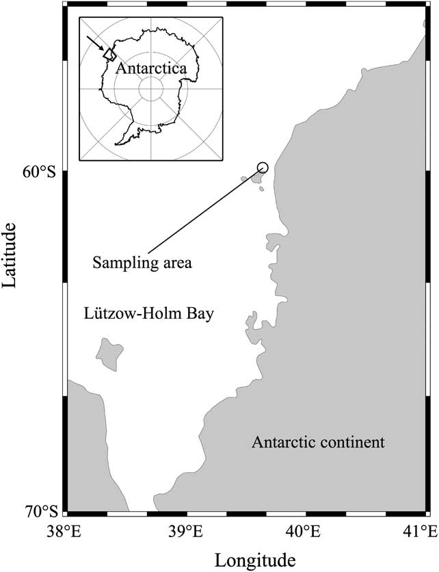
Fig. 1 Map showing the location of sampling area in Lützow-Holm Bay, East Antarctica.
For slush water sampling, snow and superimposed ice were removed with a scoop, and ice crystals in the slush layer were removed with a net. The water in the slush layer was pumped through a Teflon tube by a diaphragm pump (EWP-01, As One Corporation, Osaka, Japan) and collected in a 30 ml amber glass vial (Nichiden-Rika Glass, Kobe, Japan). Mercuric chloride solution (saturated-HgCl2; 200 μl) was added to the samples to stop biological activity. Vials were sealed with a Teflon-lined septum (Nichiden-Rika Glass) and an aluminum cap (Nichiden-Rika Glass). Slush water samples were stored in a refrigerator (+4°C) until further analysis. To check the spatial heterogeneity of slush water, duplicate samplings were carried out for slush water within 2 m2 on each sampling day.
For under-ice water sampling, a hole was made using an ice corer (Geo Tecs, Chiba, Japan) with an internal diameter of 9.0 cm, and under-ice water was collected with a Teflon water sampler (GL Science, Tokyo, Japan) at 1 m and 7 m below the bottom of the sea ice. Under-ice water samples were collected c. 30 min after drilling of the ice cores to avoid the effects of the disturbance caused by drilling. Samples were treated and stored in the same manner as for slush water samples.
The temperature of the slush and under-ice water was measured using a needle type temperature sensor (Testo 110 NTC, Brandt Instruments, Prairieville, LA, USA). Slush and under-ice water samples were also collected and placed into 12 ml glass screw-cap vials (Nichiden-Rika Glass) for salinity analysis, and into 500 ml Nalgene polycarbonate bottles (Thermo Fisher Scientific, Waltham, MA, USA) for chlorophyll a (chl a) measurement. Salinity samples were kept in a refrigerator (+4°C). The seawater samples for chl a analysis were filtered through 25 mm Whatman GF/F filters immediately after returning to the laboratory near the sampling station. Chlorophyll pigments on the filters were extracted in dimethylformamide (Suzuki & Ishimaru Reference Suzuki and Ishimaru1990) for 24 h at c. -80°C.
The bromoform concentrations were determined by a purge-and-trap (P&T) and gas chromatography-mass spectrometry (GC-MS) method (Yokouchi et al. Reference Yokouchi, Taguchi, Saito, Tohjima, Tanimoto and Mukai2006, Ooki & Yokouchi Reference Ooki and Yokouchi2011a, Reference Ooki and Yokouchi2011b). The total volume of seawater in the sample bottle was transferred to a custom-made bubbling vessel by helium carrier at 40 ml min-1. The dissolved bromoform in the water was purged with the helium carrier at 80 ml min-1 and 45°C for 30 min, and simultaneously transferred to a pre-concentration GC-MS system (Agilent 5973, 6390; Agilent Technologies, Santa Clara, CA, USA) (Yokouchi et al. Reference Yokouchi, Taguchi, Saito, Tohjima, Tanimoto and Mukai2006, Ooki & Yokouchi Reference Ooki and Yokouchi2011a, Reference Ooki and Yokouchi2011b). The purge efficiency for bromoform was 84%. A diluted standard solution containing bromoform at 1.2 pmol l-1 was introduced to the P&T GC-MS system every 24 h to calibrate for the bromoform concentrations in seawater samples. The precision of standard solution measurements was ± 2% (n = 4), and the detection limit (S/N = 10) was 0.4 pmol l-1.
Salinity was measured with a salinity analyser (SAT-210, Toa Electronics, Tokyo, Japan). The salinity analyser was calibrated with International Association for the Physical Science of the Ocean standard seawater (P series, Ocean Scientific International, Hampshire, UK). Chlorophyll a concentrations were determined using a fluorometer (Model 10AU, Turner Designs, Sunnyvale, CA, USA), following methods described by Parsons et al. (Reference Parsons, Takahashi and Hargrave1984).
Results
Bromoform and chl a concentrations, salinity and temperature
Bromoform and chl a concentrations, salinity and temperature in slush and under-ice water obtained during the study period are summarized in Table I. The mean bromoform concentration in slush water was 5.5 pmol l-1, which was lower than that of under-ice water (10.9 pmol l-1). In contrast, the mean chl a concentration in slush water (0.4 μg l-1) was approximately double that of under-ice water (0.2 μg l-1). The mean salinity of the slush water (9.7) was approximately one third that of the under-ice water (32.5). The mean temperature of the slush water (+0.5°C) was higher than that of the under-ice water (-0.4°C) due to the downward flushing of meltwater from the top, which was generated by the melting of the snow on sea ice at higher air temperature (Fig. 2). Although the range of values for some of these parameters includes temporal variations during the study period, the slush water was consistently characterized by lower bromoform concentrations and lower salinity compared to the under-ice water (Table I).
Table I Mean, minimum, Q1 (25 percentile), median, Q3 (75 percentile) and maximum of bromoform and chl a concentrations, and salinity and temperature for slush water (n = 22) and under-ice water (n = 30–32) as measured during the study period.
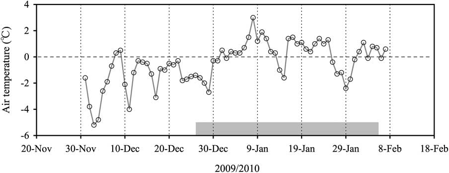
Fig. 2 Time series of daily mean air temperatures at the sampling station. Gray band indicates the sampling period.
Temporal variations in bromoform and chl a concentrations, salinity and temperature
Sampling occurred from late spring (26 December) to midsummer (5 February), providing an opportunity to observe temporal variations of physico-chemical properties during warming and ice melting conditions (Fig. 2). The snow depth over the sea ice decreased from 100 cm at the beginning of this period to less than 10 cm at the end, whereas ice thickness was almost constant during the period (176 ± 25 cm). There was a layer of superimposed ice (around 10 cm thick) between the snow and slush layers during the sampling period.
Temporal variations in bromoform and chl a concentration, salinity and temperature in slush and under-ice water are shown in Fig. 3. Bromoform concentrations in the slush water were relatively constant (8–9 pmol l-1) until 5 January, and then they decreased to below 5 pmol l-1 and remained constant for the rest of the sampling period (Fig. 3a). The salinity of the slush water decreased dramatically from 28.6 on 26 December to 0.8 on 2 February (Fig. 3e). On the other hand, the slush water temperature increased from -1.9°C to +2.6°C during the study period (Fig. 3g). The trends of decrease in salinity and increase in temperature of slush water were similar to that of bromoform concentrations during this period (Fig. 3a, e & g), with the bromoform concentrations being correlated with the salinity (shown in Fig. 4), and with the temperature of slush water (r = 0.78, P < 0.0001, n = 22). For the relationship between salinity and bromoform concentrations in slush water (Fig. 4), there were two different regimes: 1) the decrease in bromoform concentrations in the slush water only holds until a decrease in salinity to around 5, 2) at lower salinity (salinity < 5), the bromoform concentration in slush water increased to 5.9 pmol l-1 with decreasing salinity. Chlorophyll a concentrations in slush water varied between 0.0 and 1.1 μg l-1 (Fig. 3c), and were not correlated with the changes in bromoform concentrations (r = 0.09, P = 0.68, n = 22).
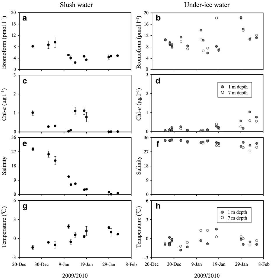
Fig. 3 Time series values for a. & b. bromoform concentration, c. & d. chl a concentration, e. & f. salinity, and g. & h. temperature, for slush water (a, c, e & g) and under-ice water (b, d, f & h). Error bars for slush water data (a, c, e & g) indicate the range of duplicate measurements. Error bars are only shown if they extend beyond the symbols.
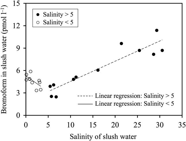
Fig. 4 Relationships between salinity and bromoform concentrations in slush water. Solid and dashed line represents the linear regression line. Bromoform concentrations in slush water were correlated with the salinity in slush water for salinity > 5 (r = 0.93, P < 0.0001, n = 12) and for salinity < 5 (r = 0.64, P < 0.046, n = 10).
Concentrations of bromoform in under-ice water (5–18 pmol l-1) were higher compared with the slush water concentrations (Fig. 3a & b). Chlorophyll a concentrations in under-ice water remained low (< 0.3 pmol l-1) until 14 January, and then they gradually increased (Fig. 3d). Salinity of under-ice water decreased from around 34 early in the study period (26 December–5 January) to below 30 at the end (29 January–5 February) (Fig. 3f). The temperature of under-ice water increased slightly during the study period (Fig. 3h). There were no notable differences between the under-ice water at 1 m and 7 m for any of the parameters during the study period (Fig. 3b, d, f & h).
Discussion
The bromoform concentrations in under-ice water measured in this study (5.9–18.3 pmol l-1) were lower than those of Arctic under-ice water in spring (around 80 pmol l-1, Sturges et al. Reference Sturges, Cota and Buckley1997) and coastal Antarctic surface water in spring/summer (around 57 pmol l-1, Carpenter et al. Reference Carpenter, Wevill, Palmer and Michels2007). The higher bromoform concentrations previously measured in polar seawater were caused by inputs of ice meltwater containing high levels of bromoform produced by ice algae, or by in situ production of bromoform in the seawater during algae blooms (e.g. Sturges et al. Reference Sturges, Cota and Buckley1992, Carpenter et al. Reference Carpenter, Wevill, Palmer and Michels2007). The increasing levels of bromoform in the ocean have generally been associated with the increasing abundance of diatoms (Klick & Abrahamsson Reference Klick and Abrahamsson1992, Baker et al. Reference Baker, Reeves, Nightingale, Penkett, Gibb and Hatton1999). An in situ culture experiment has shown that Arctic ice algae have the potential to produce substantial quantities of bromoform at high chl a concentrations (> 700 μg l-1) within the bottom layer of sea ice (Sturges et al. Reference Sturges, Cota and Buckley1992). However, because chl a concentrations were generally low during our study (mean 0.2 μg l-1), the contribution of ice algae to bromoform production would have been minor. This is probably one of the reasons why bromoform concentrations in under-ice water in this study were so much lower than those of previous studies (Sturges et al. Reference Sturges, Cota and Buckley1992, Carpenter et al. Reference Carpenter, Wevill, Palmer and Michels2007).
A surface slush layer is found widely distributed in Antarctic sea ice during the ice melting season (Haas et al. Reference Haas, Thomas and Bareiss2001, Kattner et al. Reference Kattner, Thomas, Haas, Kennedy and Dieckmannm2004, Ackley et al. Reference Ackley, Lewis, Fritsen and Xie2008, Zemmelink et al. Reference Zemmelink, Hintsa, Houghton, Dacey and Liss2008, Papadimitriou et al. Reference Papadimitriou, Thomas, Kennedy, Kuosa and Dieckmann2009). Snow accumulation over sea ice and the formation of superimposed ice leads to the formation of a slush layer below sea level (Haas et al. Reference Haas, Thomas and Bareiss2001). In this layer, high biological activity has been found (Kattner et al. Reference Kattner, Thomas, Haas, Kennedy and Dieckmannm2004), suggesting that the biogenic production of bromoform should also be high in this layer. However, in this study we found chl a concentrations in the slush layer (mean 0.4 μg l-1, Table I) to be much lower than those in the productive slush layer in the Weddell Sea, Antarctica (3.1–16.5 μg l-1, Kattner et al. Reference Kattner, Thomas, Haas, Kennedy and Dieckmannm2004). Snow depth was basically high (mean 24 cm) compared to those in the Weddell Sea, Antarctica (mean 16 cm, Kattner et al. Reference Kattner, Thomas, Haas, Kennedy and Dieckmannm2004). These results suggest the reduction of the light intensity in the slush layer, thereby reducing the light available for growth of ice algae living in slush water. In addition, the salinity of slush water was lower than under-ice water, reflecting the dilution of all slush water components including nutrients. Therefore, it was considered that available nutrient concentration in the slush water was also low and depleted for growth of ice algae. Although measures of the light intensity and nutrient concentrations in slush layer were not examined in this study, these may be one of the factors controlling biological productivity in slush water.
The temporal decrease of bromoform concentrations in slush water was correlated with that of salinity when the salinity was higher than 5 (Fig. 4), suggesting that bromoform concentrations in the slush water decreased because of dilution by the meltwater input from the upper surface of sea ice in accordance with the increase of temperature (Figs 2 & 3g). Therefore, the decrease in bromoform concentrations in slush water should closely reflect the effects of dilution. Same dilution process was observed for hexachlorocyclohexane in sea ice brine in the Canadian western Arctic in spring due to the melting of the ice crystal matrix and replenishment of brine with seawater (Pucko et al. Reference Pucko, Stern, Macdonald and Barber2010). On the other hand, at lower salinity (salinity < 5), the bromoform concentrations in the slush water increased with decreasing salinity (Fig. 4). It is speculated that the bromoform in the slush layer tended to remain even if the large volume of meltwater was added to the slush layer and diluted the bromoform because of the limited gas diffusion to the atmosphere through the snow and superimposed ice (Delille Reference Delille2006, Nomura et al. Reference Nomura, Inoue, Toyota and Shirasawa2010).
In contrast to the changes in slush water, bromoform concentrations in under-ice water increased during the study period, tracking the increase in chl a concentrations, whereas the salinity decreased (Fig. 3b, d & f). These results for salinity suggest that the under-ice water included a proportion of meltwater from the sea ice. This phenomenon is similar to the process occurring in the slush water, but there are some differences in the effects on bromoform and chl a concentrations. Previously, bromoform and chl a concentration at the bottom of the sea ice have been found to be higher than in the other parts of sea ice (Sturges et al. Reference Sturges, Cota and Buckley1997). During ice melting, the impurities in sea ice brine channels are flushed out before the melting of the ice itself, therefore these components were added to the under-ice water with meltwater. The temporal changes of each component in under-ice water reflect the input of the high-bromoform and chl a, low-salinity meltwater during the study period (Fig. 3b, d & f). These changes would also be enhanced by the horizontal advection of under-ice water from offshore that accumulates in Lützow-Holm Bay (Ohshima et al. Reference Ohshima, Takizawa, Ushio and Kawamura1996).
Conclusions
Bromoform concentrations in slush-layer water in Antarctic fast ice were measured during the seasonal warming in Lützow-Holm Bay. Mean bromoform concentration was 5.5 ± 2.4 pmol l-1, which was lower than that of the under-ice water (10.9 ± 3.5 pmol l-1). Temporal decrease in bromoform concentrations and salinity with increasing in temperature of the slush water, suggests that bromoform concentrations in the slush water decreased because of dilution by the meltwater input from the upper surface of sea ice in accordance with the increase of temperature. However, at lower salinity of slush water (salinity < 5), the bromoform concentrations in the slush water increased with decreasing salinity. It is speculated that the bromoform in the slush layer tended to remain even if the large volume of meltwater were added to the slush layer and diluted bromoform in slush water because of the limited gas diffusion to the atmosphere through the snow and superimposed ice (Delille Reference Delille2006, Nomura et al. Reference Nomura, Inoue, Toyota and Shirasawa2010).
In contrast to the changes in slush water, bromoform concentrations in under-ice water increased during the study period, tracking the increase in chl a concentrations, whereas the salinity decreased. These results suggest that the temporal changes of each component in under-ice water reflect the input of the high-bromoform and chl a, low-salinity meltwater during the study period.
Acknowledgements
We thank Mr H. Shinagawa, Dr S.A. Chavanich, Mr H. Shimoda and all the members of the 51st Japanese Antarctic Research Expedition (JARE-51) for their support in the field. We also thank Prof T. Odate, Dr Y. Yokouchi, Dr G. Hashida and Dr T. Iida for their useful comments and for providing the measurement device (purge-and-trap GC-MS). The constructive comments of the reviewers are also gratefully acknowledged.


