


1. INTRODUCTION
The global positioning system (GPS) has seen significant modernisation including the addition of new civil signals (Fontana et al., Reference Fontana, Cheung, Novak and Stanstell2001). The characteristics of these signals are designed to improve performance in terms of greater satellite visibility (higher signal power, longer codes, pilot signals, fast acquisition, higher penetration and better interference protection); higher ranging and positioning accuracy (reduced multipath, ionospheric, orbit and clock errors) and better integrity monitoring (greater satellite visibility and signal diversity). The signal features are given in Table 1 (Fontana et al., Reference Fontana, Cheung, Novak and Stanstell2001) in terms of the signal type, carrier frequency, code length, code clock, phases, bit rate, forward error correction (FEC), ionospheric error ratio, correlation protection and constellation signal type status. Since the effect of the ionosphere is inversely proportional to the frequency squared, the effects at the GPS frequencies, L2 (1227.60 MHz) and L5 (1176.45 MHz) are 65% and 79% respectively, higher than the L1 frequency at 1575.42 MHz. Since L2 has the longest code, it should give the best correlation protection, while L1 with the shortest code should give the worst. This property is vital for situations where some satellite signals are strong and others are very weak for positioning in difficult environments. Furthermore, the long code should enable L2C receivers to reject narrowband interference signals.
Table 1. Characteristics of the L1, L2 and L5 signals (Fontana et al., Reference Fontana, Cheung, Novak and Stanstell2001).

A useful approach is to compare the three civil signals (L1 C/A, L2C and L5 code) taking the legacy L1 C/A code as a reference (Fontana et al., Reference Fontana, Cheung, Novak and Stanstell2001). The comparison in Table 2 is in terms of the total received signal power, channel power, data modulation capability and effectiveness for carrier tracking. In terms of total received signal power, L5 is the strongest signal, at 3.7 dB above the L1 C/A. L2C is the weakest, at 2·3 dB below L1 C/A. The L2C and L5 signals have two components, with and without data. Each of the components of the L5 signal has a higher power than L1 C/A, whereas each of the components of L2C is considerably less.
Table 2. Comparison of L1 C/A, L2C and L5 signals (Fontana et al., Reference Fontana, Cheung, Novak and Stanstell2001).

Comparing the relative channel power levels with the relative data thresholds, there is a 5 dB gain in data recovery thresholds for both L2C and L5 due to FEC. Furthermore, L2C gains another 3 dB because its bit rate is 25 bps rather than 50 bps. Adding the gains to the initial relative channel power (5·3 dB below), results in L2C being 2·7 dB better in the data recovery threshold than L1 C/A. Similarly, comparing the relative channel power levels with the relative carrier tracking threshold, there is a 6 dB gain in the carrier tracking threshold offered by a phase locked loop employed in L2C over a Costas loop (used in L1/CA). Adding this gain to the initial relative channel power (5·3 dB below) results in L2C being 0·7 dB better than L1 C/A in carrier tracking. Since L5 has 6 dB more power than L2C, it has the best carrier tracking capability of the three civil signals.
Several researchers have investigated the impact of the new signals (Tran, Reference Tran2004; Sükeová et al., Reference Sükeová, Santos, Langley, Leandro, Nnani and Nievinski2007; Engel, Reference Engel2008; Cai et al., Reference Cai, He, Santerre, Pan, Cui and Zhu2016; Saleem et al., Reference Saleem, Usman, Elahi and Gul2017). The research to date has focussed on measurement quality in terms of signal strength and precision for static applications using either simulated or real data captured in open and clean environments represented by the reference stations, such as those operated by the International GNSS Service (IGS). The results have variously shown different levels of improvements of the L5 signal over the L1 and L2 signals with respect to signal strength and code measurement precision. Furthermore, Sükeová et al. (Reference Sükeová, Santos, Langley, Leandro, Nnani and Nievinski2007) suggested that the strength of the L2 signal on the modernised satellites is higher than that of the legacy L2 signal. Therefore, to date there has been no comprehensive research to characterise the performance in the built environment for dynamic applications such as the location based services to be provided by intelligent transport systems for bus operations. Such services are required to improve the efficiency of bus operations to increase ridership thereby reducing congestion, delays and pollution within cities (UN, 2017, 2018). Table 3 lists the location based services and their required positioning accuracy resolved into the along track and cross track components (Elhajj, Reference Elhajj2017). Furthermore, research on the impact of the new signals on positioning measured in terms of the required navigation performance parameters of accuracy, integrity, continuity and availability has been patchy due to a lack of enough satellites in the constellation transmitting the new signals, for both static and dynamic applications in all environments. This paper addresses these gaps with a focus on measurement precision and positioning accuracy.
Table 3. Required positioning accuracy for urban bus location based services.

The rest of this paper is structured as follows. Section 2 presents the performance assessment process. This is followed in Sections 3 and 4 by the methodologies adopted for the measurement and position domain analyses respectively. The corresponding results are presented and discussed in Section 5 before the paper is concluded in Section 6.
2. PERFORMANCE CHARACTERISATION PROCESS AND DATA
To capture the impacts of the design features of the new GPS signals, the performance analysis is undertaken in both the measurement and position domains. The former essentially quantifies signal quality in two ways. First, it analyses signal-to-noise ratio (SNR) data. SNR is the ratio of the signal power and noise power in a given bandwidth and is an indication of the level of noise present in a measurement. Second, the analysis uses multiple frequency data to account for the ionospheric error and quantify measurement precision by determining the level of multipath and noise in the legacy (L1 C/A) and new (L2C and L5) ranging codes.
In the positioning domain, positioning accuracy is quantified with a focus on the mitigation of the ionosphere error using L1 C/A and L2C measurements. At the time of this research there were 19 and 15 satellites broadcasting the L2C and L5 signals respectively. Unfortunately, because of the relatively low number of L5 broadcasting satellites, position domain analysis with the L5 code data is not attempted. Improvement is demonstrated only through improved precision, as shown by the level of multipath and noise in the L5 code measurements.
The analysis is undertaken with static and dynamic data. The static data are gathered at the IGS reference station BRUX in Belgium operating a Septentrio POLARX4TR receiver capable of generating all the legacy and new signals. The dynamic data were captured in London (Figure 1) using an instrumented vehicle (Figure 2). The vehicle followed a route from Imperial College London in South Kensington via Westminster to Canary Wharf and back to Imperial College (Figure 1), largely representing a mix of ‘fair’ and ‘poor’ conditions for positioning. One high grade GNSS/IMU sensor (from iMAR, Figure 3) was used together with the Leica GS15 multi-frequency multi-constellation receiver and the multi-frequency NovAtel receiver OEM6 receiver (NovAtel, 2016). The data were sampled at 1 Hz.

Figure 1. Aerial view of London showing route from Imperial College to Canary Wharf and back to Imperial College.

Figure 2. Receiver antennae configuration.

Figure 3. iMAR GNSS/IMU Sensor.
3. MEASUREMENT DOMAIN ANALYSIS METHODOLOGY
The measurement domain analysis is undertaken in two ways. The first involves the assessment of the SNR of the L1, L2 and L5 signals generated by the receiver. The second approach analyses the level of multipath and noise.
3.1. SNR
The methodology adopted for the analysis of SNR data considers representative legacy and modernised satellites. The SNR data from static and dynamic (urban) data from different receivers are processed to generate SNR distributions in 5 dB-Hz statistical bins.
3.2. Multipath and noise
Except for the ionospheric effect, the main distinguishing features of the civil signals relate to multipath and noise. As the effect of the ionosphere is deterministic, accountable through dual frequency measurements, it is possible to quantify the effects of multipath and noise in a given pseudorange measurement by a combination of pseudorange and carrier phase measurements (Sükeová et al., Reference Sükeová, Santos, Langley, Leandro, Nnani and Nievinski2007).
The observation equation for each pseudorange for a given frequency i and a satellite-receiver pair are:
 $$\mbox{PR}_i =\rho -c\delta \tau +c\delta t+d_{{\rm orb}} +d_{{\rm ion}_i }+d_{{\rm trp}} +d_{{\rm mp}_{{\rm pri}} } +d_{{\rm nse}_{{\rm pri}} }$$
where ρ is the geometric range, δ τ the receiver clock offset, δ t the satellite clock offset, d orb the satellite orbit error,  $d_{{\rm ion}_{i} } $ the ionosphric error, d trp the tropospheric delay,
  $d_{{\rm mp}_{{\rm pri}} } $ the code multipath error,
  $d_{{\rm nse}_{{\rm pri}} } $ the code noise and c is the speed of light in a vacuum.
The corresponding carrier phase observation equation is given by:
 $$\Phi _i =\rho -c\delta \tau +c\delta t+\lambda _i N_i + d_{{\rm orb}} -d_{{\rm ion}_i } +d_{{\rm trp}} + d_{{\rm mp}_{\Phi i} } +d_{{\rm nse}_{\Phi i} }$$
where λi is the wavelength of the carrier frequency, N i the initial integer ambiguity,  $d_{{\rm mp}_{\Phi i}}$ the carrier multipath and
  $d_{{\rm nse}_{\Phi i} } $ the carrier phase noise.
Exploiting the fact that the level of multipath and noise in the carrier phase measurement is significantly lower than in the code pseudorange measurements, the difference between the pseudorange and carrier phase measurements for satellite i is expressed as:
 $$\mbox{PR}_i -\Phi _i =2d_{{\rm ion}_i } -\lambda _i N_i +d_{{\rm mp}_{{\rm PRi}} } +d_{{\rm nse}_{{\rm PRi}} } -d_{{\rm mp}_{\Phi i} } -d_{nse_{\Phi i} }$$
 Ignoring receiver hardware delays, Equation (3) has eliminated the common errors due to the receiver clock, satellite clock, satellite orbit and the troposphere. To access the pseudorange multipath and noise, the ionospheric error  $( d_{{\rm ion}_{i} } ) $ in Equation (3) must be eliminated.
As the effect of the ioniosphere is inversely proportional to the frequency (\underline {f}) squared, the relationship between the delays on two different frequencies (e.g., L1 and L2) is:
 $$d_{{\rm ion}_2 } =d_{{\rm ion}_i } \frac{f_1^2 }{f_2^2 }$$
The difference of carrier phase observations on two frequencies (e.g., L1 and L2) yields:
 $$\Phi _2 -\Phi _1 =d_{{\rm ion}_{1}} -d_{{\rm ion}_{2} } + \lambda _2 N_2 -\lambda _1 N_1 +d_{{\rm mp}_{\Phi 2} } -d_{{\rm mp}_{\Phi 1} } +d_{{\rm nse}_{\Phi 2} } -d_{{\rm nse}_{\Phi 1} }$$
 Substituting  $d_{{\rm ion}_{2} } $in Equation (4) into Equation (5), yields the ionospheric delay in L1 frequency as:
 $$d_{{\rm ion}_1 } =\left( {\frac{f_2^2 }{f_1^2 -f_2^2 }}\right)\left( {\Phi _1 -\Phi _2 +\lambda _2 N_2 -\lambda _1 N_1+d_{{\rm mp}_{\Phi 2} } -d_{{\rm mp}_{\Phi 1} } +d_{{\rm nse}_{\Phi 2} }-d_{{\rm nse}_{\Phi 1} } } \right)$$
Substituting Equation (6) into Equation (3), for example, for the L1 and L2 frequencies yields:
 $$\begin{align} \mbox{PR}_1 -\Phi_1 &=2\left\{ {\left( {\frac{f_2^2 }{f_1^2 -f_2^2 }}\right)\left( {\Phi _1 -\Phi _2 +\lambda _2 N_2 -\lambda _1 N_1+d_{{\rm mp}\Phi _2 } -d_{{\rm mp}_{\Phi 1} } +d_{{\rm nse}_{\Phi 2} }-d_{{\rm nse}_{\Phi 1} } } \right)} \right\} \\ & \quad-\lambda _1 N_1 +d_{{\rm mp}_{{\rm PR}1} } +d_{{\rm nse}_{{\rm PR}1}} -d_{{\rm mp}_{\Phi 1} } -d_{{\rm nse}_{\Phi 1} }\end{align}$$
Ignoring carrier phase measurement multipath errors and noise in Equation (7), and rearranging yields:
 $$\begin{align} d_{{\rm mp}_{{\rm PR1}} } +d_{{\rm nse}_{{\rm PR1}} } &=\mbox{PR}_1 -\left( {\frac{f_1^2 +f_2^2 }{f_1^2 -f_2^2 }} \right)\Phi _1 +\left( {\frac{2f_2^2 }{f_1^2 -f_2^2 }} \right)\Phi _2\nonumber\\ &\quad +\left\{ {\left( {\frac{f_1^2 +f_2^2 }{f_1^2 -f_2^2 }} \right)( {\lambda_1 N_1 } ) -\left( {\frac{2f_2^2 }{f_1^2 -f_2^2 }} \right)( {\lambda_2 N_2 } ) } \right\} \end{align}$$
As can be seen from Equation (8), its right side has a constant part due to the integer ambiguities. Therefore, generalising for carrier frequencies i and j results in:
 $$\begin{align} d_{{\rm mp}_{{\rm pri}} } +d_{{\rm nse}_i } &=\mbox{PR}_i -\left( {\frac{f_i^2 +f_j^2 }{f_i^2 -f_j^2 }} \right)\Phi _i +\left( {\frac{2f_j^2 }{f_i^2 -f_j^2 }} \right)\Phi _j\nonumber\\ &\quad -\left\{ {\left( {\frac{f_i^2 +f_j^2 }{f_i^2 -f_j^2 }} \right)( {\lambda_i N_i } ) -\left( {\frac{2f_j^2 }{f_i^2 -f_j^2 }} \right)( {\lambda_j N_j } ) } \right\} \end{align}$$
Assuming that other deterministic error terms such as hardware delays are absorbed in the ambiguity parameters, given a series of measurements and cycle slip detection, the mean represents the constant ambiguity term. This is computed using the simple averaging technique presented in the next sub-section and removed to reveal the level of multipath and noise in the pseudorange measurements.
3.2.1. Cycle slips in carrier phase measurements
Cycle slips (jumps or discontinuities in the carrier phase measurements) are caused when a receiver loses lock on a signal. These jumps introduce error in the position estimation and must be detected and/or corrected. A relatively simple method for the detection of cycle slips is based on the geometry-free (GF) phase observable derived from the difference between the carrier phase measurements on two frequencies, i and j in Equation (10). The GF observable removes the geometry (range), and the common errors from the satellite orbit, satellite clock, tropospheric error and receiver clock.
 $$\Phi _{{\rm GF}} =\Phi _i -\Phi _j$$
The difference across time (k) of consecutive GF observables enables cycle slips to be detected due to changes in the differenced ambiguity. In order to amplify the cycle slip, the nth order differencing can be used (at the risk of increasing noise and the potential for false detection). Normally, the second order is appropriate, as shown in Equation (11) (Sanz Subirana et al., Reference Sanz Subirana, Juan Zornoza and Hernandez-Pajares2013). A threshold for the detection of cycle slips is required taking into account the noise characteristics of the time differenced observable.
 $$\Delta \Phi _{{\rm GF}} =(\Phi _{{\rm GF}_k } -\Phi _{GF_{k-1} } )-(\Phi_{GF_{k-1} } -\Phi _{GF_{k-2} } )$$
To determine the constant ambiguity term in Equation (9), in post-processing, the simple averaging technique in Equation (12) can be used for n previous measurements before a cycle slip is detected. The process is reset when a cycle slip is detected and cannot be repaired.
 $$\begin{align} \left\{ {\left( {\frac{f_i^2 +f_j^2 }{f_i^2 -f_j^2 }} \right)( {\lambda_i N_i } ) +\left( {\frac{2f_j^2 }{f_i^2 -f_j^2 }} \right)( {\lambda_j N_j } ) } \right\}_n =\frac{\sum\nolimits_1^n {\left\{{\mbox{PR}_i -\left( {\frac{f_i^2 +f_j^2 }{f_i^2 -f_j^2 }} \right)\Phi_i +\left( {\frac{2f_j^2 }{f_i^2 -f_j^2 }} \right)\Phi_j } \right\}_n } }{n} \end{align}$$
If cycle slip correction is applied in real-time, a cumulative averaging technique can be used.
4. MEASUREMENT DOMAIN RESULTS AND ANALYSIS
4.1. SNR
The distribution of the SNR for the dynamic data captured in the urban environment for the legacy satellites (represented by satellites G02 and G14) is shown in Figures 4 and 5 respectively. It is clear that the L1 signal exhibits a higher SNR than the L2 signal.

Figure 4. G02 L1 and L2 SNR.

Figure 5. G14 L1 and L2 SNR.
The distribution of SNR for the modernised satellites broadcasting the L1 and L2 signals (represented by satellites G07 and G15) is presented in Figures 6 and 7 respectively). Again the L1 signal has a higher SNR than the L2 signal, with no indication that the L2 SNR for the legacy satellites is significantly different from the modernised satellites. This suggests no appreciable difference in the signal strength between the L2 signals from the legacy (old) and modernised (new) satellites.

Figure 6. G07 L1 and L2 SNR.

Figure 7. G15 L1 and L2 SNR.
The distribution of the SNR data for the new satellites broadcasting all the three signals (represented by satellites G01 and G26) is shown in Figures 8 and 9 respectively. While confirming the previous results that the L1 signal has a higher SNR than the L2 signal, the L5 signal has the highest SNR of all three.

Figure 8. G01 L, L2 and L5 SNR.

Figure 9. G26 L, L2 and L5 SNR.
The results for the static IGS station BRUX exhibit similar relative performance. The next section analyses the level of multipath and noise in the L1 C/A, L2C and L5 code measurements, and determines if the SNR is indeed reflective of the existence of and level of multipath and noise.
4.2. Multipath and noise
Considering the frequencies of the three signals and accounting for the need to remove the effects of the ionosphere, the best combinations for the estimation of code multipath and noise are L1/L2 and L1/L5, due to the larger differences between the sets of frequencies. Based on this Figures 10 and 11 present the multipath and noise in L1 C/A, L2C and L5 code measurements for satellites G01 and G09 respectively, from the data captured by the Septentrio receiver at the IGS station BRUX. The corresponding average, standard deviation (SD) and root mean square (RMS) values are presented in Table 4.

Figure 10. G01 – code multipath and noise.

Figure 11. G09 – code multipath and noise.
Table 4. L1 C/A, L2C and L5 code multipath and noise statistics.

From the results in Table 4, although the RMS values are different (because of the differences in the sample size and the effects of elevation), there is a level of consistency in the relative levels of multipath and noise in the code measurements. Furthermore, the RMS multipath and noise values are lowest for the L5 code (0·203/0·200 m), followed by the L1 C/A (0·296/0·221 m) and highest for L2C (0·307/0·248 m). Note that the mean is included here to demonstrate that the constant ambiguity term has been determined correctly.
The results for the dynamic London data for L1C/A, L2C and L5 code measurements are given in Figures 12 and 13 for satellites G30 and G32, with summary statistics in Table 5.

Figure 12. G30 – code multipath and noise.

Figure 13. G32 – code multipath and noise.
Table 5. New satellites multipath and noise statistics (L1 C/A, L2C and L5 codes).

From the results in Figures 12 and 13, and Table 5, the following observations can be made. First, the levels of multipath and noise (in terms of RMS) in the L1 C/A code measurements are 0·309 m and 0·401 m. The corresponding values for the L2C code measurements are 1·070 m and 1·301 m. The corresponding values for the L5 code measurements are 0·147 m and 0·368 m. Second, the levels of multipath and noise in the L1 C/A code measurements are always lower than in the L2C code measurements. Third, the level of multipath in the L5 code measurements is always lower than the L1 C/A measurements.
In summary, both for clear and built environments, L5 code measurements have the lowest level of multipath and noise, followed by L1 C/A, with L2C the highest. Furthermore, the level of multipath and noise is in general higher in the built environment than the clear open environment due to higher signal attenuation in the former.
5. POSITION DOMAIN METHODOLOGY, RESULTS AND ANALYSIS
This section quantifies the impact of the L1 C/A and L2C code measurements on position accuracy, with a particular focus on the mitigation of the effects of the ionosphere. In the same way as in the measurement domain, the position domain analysis is carried out with data from the static IGS station BRUX and dynamic data captured in London. The generic elements of the positioning solution are presented in Table 6, with the specifics discussed within each analysis scenario.
Table 6. Generic position solution elements.

5.1. Static data
Given that, at the time of writing, there are only 19 satellites broadcasting the L2C signal, their impact on the positioning accuracy is analysed as captured in the scenarios presented in Table 7, including the rationale for each.
Table 7. L2C impact analysis scenarios.

5.1.1. Comparison of scenarios 1 and 2
Figures 14 and 15 and Table 8 compare the 3D positioning error results computed from the differences between the least squares solutions and the published known coordinates of the BRUX IGS station. Figure 14 presents the 3D position errors for the two cases when only the L1 C/A code pseudoranges are used, and when the available L2C pseudoranges are included to generate dual frequency solutions, without the application of the Klobuchar model where relevant. The corresponding probability density function (pdf) and cumulative distribution function (cdf) are presented in Figure 15. Table 8 presents the main statistical results at the 67th and 95th percentiles, mean, SD and RMS error (RMSE).

Figure 14. 3D position error (L1C/A_NO_IONO and L1C/A_L2C_NO_KLOB).

Figure 15. Position error pdf and cdf (L1C/A_NO_IONO and L1C/A_L2C_NO_KLOB).
Table 8. 3D position error statistics (L1C/A_NO_IONO and L1C/A_L2C_NO_KLOB).

From Figure 14, the benefit of the 19 satellites broadcasting the L2C signal (partial constellation) is manifest in a general improvement in the position accuracy. This observation can be seen clearly in the pdf and cdf in Figure 15 with a significant shift to the left of the L1C/A_L2C position errors in relation to the L1C/A case. This is confirmed by the positioning error statistics in Table 8, showing an improvement in positioning accuracy of 46%, 22% and 35% at the 67th and 95th percentile, and RMSE respectively.
5.1.2. Comparison of scenarios 1 and 3
Having established that users can already benefit from the 19 satellites broadcasting the L2C signal, it is interesting to see if the inclusion of the L2P2 pseudoranges from the legacy satellites (that do not broadcast the L2C signal) could provide an indication of the overall level of improvement to be expected from a full constellation broadcasting the L2C signal. This approach is justified at three levels. The first is that the SNR analysis revealed no significant differences between the L2 signal broadcast by the legacy and modernised satellites. Second, measurement domain analysis showed similar levels of multipath and noise in the L2C and L2P2 pseudoranges. Third, as can be seen in Figure 16 and Table 9, the levels of performance for scenario 3 (L1/CA_L2C_L2P2) and scenario 4 (L1C/A_P2) are very close (at the decimetre level).

Figure 16. Position error pdf and cdf (L1C/A_L2C_L2P2 and L1C/A_L2P2).
Table 9. 3D position error statistics (L1C/A_L2C_L2P2 and L1C/A_L2P2).

Following the justification of the inclusion of the L2P2 pseudorange measurements as a proxy for the L2C pseudoranges for the legacy satellites, the results for the 3D position errors for scenario 1 (L1C/A_NO_IONO) and scenario 3 (L1C/A_L2C_L2P2), are presented in Figures 17 and 18 and Table 10. Figure 17 presents the 3D position errors for the two cases when only the L1 C/A code pseudoranges are used, and when the available L2C pseudoranges are augmented with the L2P2 pseudoranges to generate dual frequency solutions for the full constellation. The corresponding 3D position error pdf and cdf are presented in Figure 18. The main statistical results in terms of the 67th and 95th percentiles, mean, SD and RMSE are presented in Table 10.

Figure 17. 3D position error (L1C/A_NO_IONO and L1C/A_L2C_L2P2).

Figure 18. Position error pdf and cdf (BRUX: L1C/A_NO_IONO and L1C/A_L2C_L2P2).
Table 10. 3D position error statistics (BRUX: L1C/A_NO_IONO and L1C/A_L2C_L2P2).

From Figure 17 the benefit of the dual frequency solutions from the full constellation is seen in the improvement in positioning accuracy, compared with the single frequency (L1 C/A code only solutions). This is reflected in the pdf and cdf in Figure 18 exhibiting a larger shift to the left compared with Figure 15. The position error statistics in Table 10 show improvements of 59% and 34% at the 67th and 95th percentiles, 54% in the mean position error and 47% in the RMSE. Compared with the partial L2C constellation (brackets in Table 10), the full constellation offers a further improvement of about 13%.
To provide a complete picture of the relevant five scenarios in Table 7, Figure 19 presents the corresponding pdfs and cdfs, with the position error statistics in Table 11. From the results, three points are noticeable. First, the benefits of the full constellation over the L1 C/A single frequency with the Klobuchar model are at the levels of 25% (67%), 0% (95th percentile), 14% (mean) and 11% (RMSE). These results suggest that the Klobuchar model was effective in accounting for the effects of the ionospheric delay at this IGS station located in the mid latitude region. Second, there is no significant benefit of the partial L2C constellation over the exclusive use of the Klobuchar model with L1 C/A code pseudorange measurements. Third, the highest impact is from the full constellation.
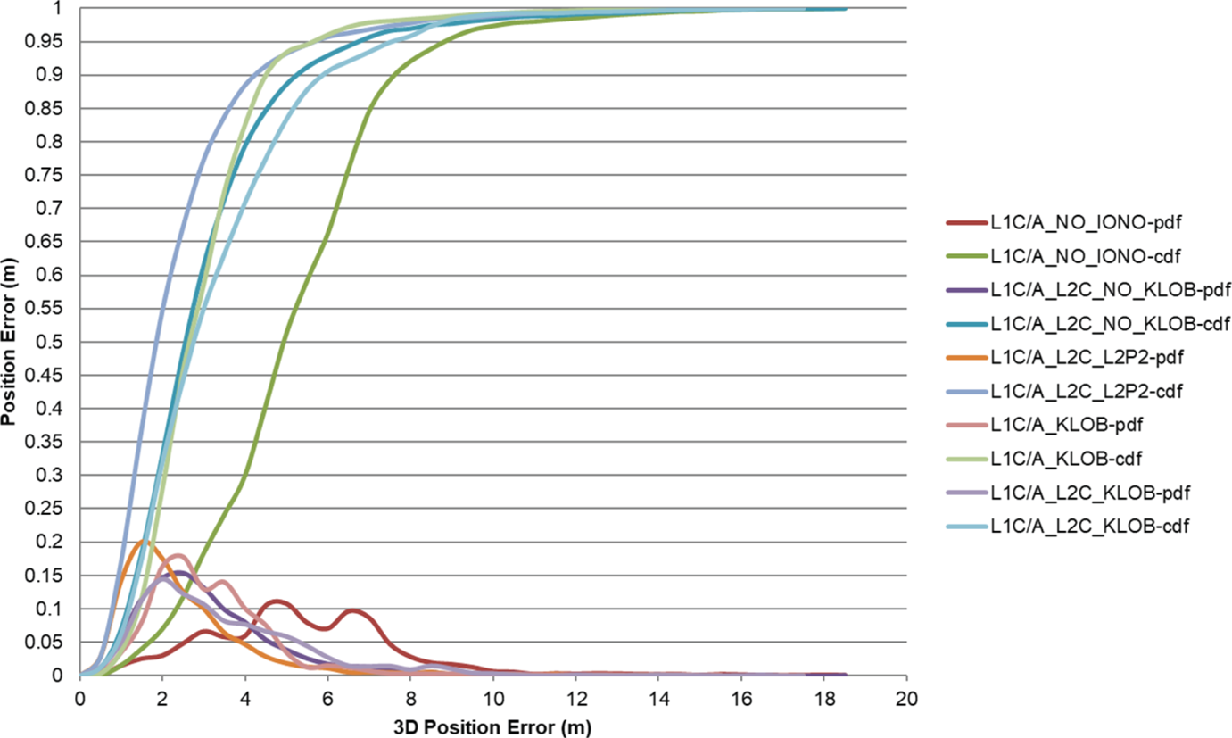
Figure 19. Position error pdf and cdf (BRUX – all five scenarios).
Table 11. 3D position error statistics (BRUX - all five scenarios).

5.2. Dynamic data
To quantify the performance from the dynamic data in London, first, a decimetre level positioning accuracy reference trajectory was generated. Inertial Explorer software was used together with dual frequency GPS and IMU data from the iMAR sensor integrated in the measurement domain. With the exception of the ionospheric error accounted for by the use of dual frequency carrier phase measurements, the other spatially correlated errors were accounted for through the use of the double differenced carrier phase observable using proximate Ordnance Survey reference stations. The Saastamoinen model was employed to account for the tropospheric delay while multipath and noise were accounted for by filtering in both directions to improve accuracy.
5.2.1. Comparison of scenarios 1 and 3
In order to capture the impact of the L2C code measurements on the positioning accuracy as a result of mitigating the effect of the ionosphere when used in combination with the L1 C/A code measurements, it is vital to account for multipath as the other dominant error in the urban environment. The Leica receiver uses a proprietary smoothing function that results in residual multipath and noise error at the decimetre level. For this reason, the Leica receiver data were processed and compared with the reference trajectory to generate the 3D and horizontal positioning errors. A threshold Position Dilution of Precision (PDOP) of 5 is used as an appropriate geometry for positioning. Figure 20 presents the pdfs and cdfs of the 3D positioning error for L1 C/A code solutions without the application of any ionospheric delay mitigation technique (scenario 1) and the dual frequency solutions of the full constellation of L1 C/A and L2C code measurements, augmented with the L2 P2 measurements (scenario 3). The benefit of the dual frequency solutions from the full constellation can be seen in the corresponding pdf and cdf in Figure 20 exhibiting a shift to the left of the pdf and cdf for the single frequency L1 C/A solution. The position error statistics in Table 12, show improvements of 8% and 48% at the 67th and 95th percentiles, 24% in the mean position error and 32% in the RMSE.

Figure 20. 3D position error pdf and cdf (scenarios 1 and 3).
Table 12. 3D position error statistics (L1C/A_NO_IONO and L1C/A_L2C_L2P2).

The horizontal position error statistics are presented in Table 13, in terms of the 95th percentile accuracy and RMSE. It can be seen that the use of the ionospherically-free linear combination of L1 C/A and L2C code measurements results in improvement at the levels of 39% in the accuracy and 23% in the RMSE. These percentage levels of improvement, although significant, are less than the 3D positioning case due to the high sensitivity of GNSS to vertical errors due to a generally weaker geometric configuration compared with horizontal positioning.
Table 13. Horizontal position error statistics (L1C/A_NO_IONO and L1C/A_L2C_L2P2).

5.2.2 Comparison of scenarios 1, 3 and 5
Figure 21 presents the pdfs and cdfs for the single frequency L1 C/A code solutions without ionospheric correction, dual frequency full constellation solutions and single frequency CA code solutions employing the broadcast (Klobuchar) model for ionospheric delay mitigation. The summary statistics are presented in Table 14. Note that although the application of the Klobuchar model results in a higher positioning accuracy than the dual frequency solution at the 67th percentile, the latter is superior at the higher percentiles (e.g. >28% improvement at the 95th percentile).

Figure 21. 3D position error pdf and cdf (Leica – scenarios 1, 3 and 5).
Table 14. 3D position error statistics (L1C/A_NO_IONO, L1C/A_L2C_L2P2 and L1C/A_IONO_KLOB).

Table 15 presents the horizontal positioning error at the 95th percentile and in terms of the RMSE. It can be seen that although the level of improvement over the single frequency C/A code based solution is reduced, the ionospherically-free position solution is still superior to the case when the Klobuchar model is applied. Compared with the single frequency C/A code based solution without correction for the ionospheric error, the improvement over the application of the Klobuchar is reduced to 15% for horizontal accuracy at the 95th percentile, and 11% in the RMSE.
Table 15. Horizontal position error statistics (L1/CA_NO_IONO, L1/CA_L2C_L2P2 and L1/CA_IONO_KLOB).

5.2.3. Partial L2C constellation
The partial constellation of only the L2C broadcasting satellites are generated by decimating the full constellation using TEQC software (unavco.org). The results for the single frequency L1 C/A code solution with no ionospheric delay correction and with the application of the Klobuchar model are compared with the use of the ionospherically-free linear combination of the L1 C/A and L2C code measurements. Figure 22 presents the pdfs and cdfs of the 3D positioning error for L1 C/A with and without the application of ionospheric delay mitigation technique, and the dual frequency (L1 C/A/L2C) solutions for the partial constellation of L1 C/A and L2C code measurements.

Figure 22. 3D position error pdf and cdf (partial constellation, L1_CA_NO_IONO, L1_CA_L2C and L1_CA_IONO_KLOB).
The benefit of the dual frequency solutions from the partial constellation is seen in the corresponding pdf and cdf in Figure 22 exhibiting largely a shift to the left of the pdf and cdf for the single frequency L1 C/A solution, particularly at the higher percentiles (greater than 85%). As in the full constellation case, although the application of the Klobuchar model generates the best results at the lower percentiles, the dual frequency solution is best at the higher percentiles. Table 16 presents the 3D position error statistics at the 67th and 95th percentiles, plus the RMSE, mean and SD.
Table 16. Partial L2C constellation 3D position error statistics (Leica: L1C/A_NO_IONO, L1C/A_L2C and L1C/A_IONO_KLOB).

A similar picture emerges when the results in Table 16 are compared with Table 14. First, there is a general improvement in the performance from the ionospherically-free linear combination compared with the single frequency C/A code solution without ionospheric delay correction. The improvements are 4% at the 67th percentile, 49% at the 95th percentile, 8% in the mean, 14% in the SD and 13% in terms of RMSE. Second, it is interesting to note that the application of the broadcast Klobuchar model results in a higher positioning accuracy than the dual frequency solution at the 67th percentile (13% better), while the latter is superior at the higher percentiles (an improvement of more than 39% at the 95th percentile), with an overall improvement in the RMSE of 10%.
6. CONCLUSIONS
This paper has analysed the impact of the new GPS signals on positioning accuracy for dynamic applications in urban environments. Static data captured in a clean environment have also been analysed to appreciate the challenges of positioning in the built environment. The analysis has been undertaken in the measurement and positioning domains. The former has analysed measurement quality as reflected in the SNR and multipath and noise in the three code phase signals L1 C/A, L2C and L5. The position domain analysis focussed on the benefit of the combined use of L1 C/A and L2C in the mitigation of the ionospheric error.
The results from the SNR analysis show that the L5 signal has the highest signal power, followed by L1, with the L2 the weakest. There is no evidence of a significant difference in SNR between the L2 signals broadcast by the old and modernised satellites. In line with the results of the relative SNR performance, the results have also shown that L5 code measurements have the least multipath and noise followed by L1 C/A, with the L2C the highest.
In the position domain, from the results of the static data captured at IGS reference stations, representing clean (with respect to multipath) and clear (unobstructed) environments, it is concluded that a full L2C constellation has the potential to improve 3D positioning accuracy compared to the case of single frequency code phase measurements without ionospheric corrections by 59% to better than 2·5 m (1σ), and 34% to about 6 m (2σ). The mean 3D positioning error is improved by 54% to better than 2·4 m with a SD better than 1·9 m, while the RMSE is improved by 47% to better than 3 m. From the dynamic urban data results, where multipath and signal blockage are particular concerns, the corresponding improvements are lower by 8% to around 5·89 m (1σ), and 48% to 13·66 m (2σ). The mean 3D positioning error is improved by 24% to 5·94 with a SD of 5·74 m, while the RMSE is improved by 32% to 8·26 m. In terms of horizontal positioning error, the use of the L1 C/A-L2C ionospherically-free liner combination results in positioning accuracy of 9·03 m (2σ), an improvement of 39% over the C/A code based solution without ionospheric error correction. The RMSE for the horizontal positioning is 5·52 m, an improvement of 23%. These improvements have the potential to benefit some of the location based services in Table 3. However, the more stringent requirements will require the direct use of the carrier phase measurements.
ACKNOWLEDGEMENTS
The assistance received from the following is acknowledged: Dr Shaojun Feng (data capture), Dr Xin Zhang and Mr Zhenjun Zhang (aspects of software development) and Dr Manela Mauro of Transport for London (data capture and location based services for bus operations). This work was supported by a scholarship from Imperial College London.


