


1. Introduction
The tendency of particles to aggregate while interacting with fluid flows, termed clustering, is evident in countless situations, including atmospheric clouds, fluidized bed reactors, swimming micro-organisms, just to name a few. Here, we focus on the classic case of small heavy particles in turbulence, which are known to cluster when their response time is comparable to the time scale of the flow. This phenomenon has attracted the attention of the fluid mechanics community for decades (Eaton & Fessler Reference Eaton and Fessler1994; Monchaux, Bourgoin & Cartellier Reference Monchaux, Bourgoin and Cartellier2012). This is justified by the potentially important role played by clusters in triggering and enhancing the interaction between particles, as well as their collective backreaction on the carrier fluid. As such, significant effort has gone into quantitatively characterizing clustering, with tools ranging from box-counting (Aliseda et al. Reference Aliseda, Cartellier, Hainaux and Lasheras2002), to radial distribution functions (Sundaram & Collins Reference Sundaram and Collins1997) and advanced topological descriptors (Calzavarini et al. Reference Calzavarini, Kerscher, Lohse and Toschi2008).
A method to characterize clustering that has gained increasing popularity is the Voronoï tessellation. Since its introduction to the field of particle-laden turbulence by Monchaux, Bourgoin & Cartellier (Reference Monchaux, Bourgoin and Cartellier2010), it has been widely used for both heavy particles and light bubbles (Tagawa et al. Reference Tagawa, Mercado, Prakash, Calzavarini, Sun and Lohse2012), homogeneous and wall-bounded turbulence (Wang et al. Reference Wang, Fong, Coletti, Capecelatro and Richter2019), point-like and finite-size particles (Fiabane et al. Reference Fiabane, Zimmermann, Volk, Pinton and Bourgoin2012), monodispersed and polydispersed particles (Lian, Chang & Hardalupas Reference Lian, Chang and Hardalupas2019), in one-way and two-way coupled regimes (Monchaux & Dejoan Reference Monchaux and Dejoan2017), mostly in hydrodynamically forced but also in buoyancy-driven turbulence (Zamansky et al. Reference Zamansky, Coletti, Massot and Mani2016) and even in freely sedimenting systems (Uhlmann & Doychev Reference Uhlmann and Doychev2014). An advantage of this technique is that it provides the local concentration associated with each particle (through the inverse of the Voronoï cell size), which in turn allows the identification of individual clusters as sets of neighbouring particles satisfying a threshold concentration. This feature was used by Baker et al. (Reference Baker, Frankel, Mani and Coletti2017) to show that clusters of heavy particles in homogeneous turbulence are self-similar objects with a broad range of sizes, and that they have significantly different fall speeds compared to non-clustered particles. The approach has been used to characterize individual clusters, including their shape, orientation, velocity and acceleration, in homogeneous turbulence (Petersen, Baker & Coletti Reference Petersen, Baker and Coletti2019; Momenifar & Bragg Reference Momenifar and Bragg2020) and in wall-bounded flows (Fong, Amili & Coletti Reference Fong, Amili and Coletti2019).
While the presence of clusters in particle-laden turbulence is not disputed, their origin and dynamics are still debated. The classic explanation refers to a centrifuging mechanism that pushes particles out of vortex cores and into high-strain regions (Eaton & Fessler Reference Eaton and Fessler1994). This has been challenged by alternative and not mutually compatible explanations, notably: the path-history effect (Bragg & Collins Reference Bragg and Collins2014), i.e. particles retaining memory of the flow fluctuations they experienced; and the sweep-stick mechanism (Goto & Vassilicos Reference Goto and Vassilicos2008), i.e. particles sticking to zero-acceleration points swept and clustered by large-scale motions. Naturally, information on the temporal evolution of clusters appears crucial to reach a predictive understanding of their dynamics. There is, however, a dire scarcity of such information in the literature. Rare exceptions are represented by Tagawa et al. (Reference Tagawa, Mercado, Prakash, Calzavarini, Sun and Lohse2012) and Lian et al. (Reference Lian, Chang and Hardalupas2019), who used the temporal autocorrelation of the Voronoï cell sizes to identify the time scales during which particles remain clustered. Indeed, the Voronoï tessellation method is naturally apt to obtain temporal information on clustering dynamics. This was one of the original motivations of Monchaux et al. (Reference Monchaux, Bourgoin and Cartellier2010), who already showed the feasibility of tracking the cell area along particle trajectories.
To date, no study has addressed the temporal evolution of individual clusters, nor investigated systematically their lifecycle. As such, several fundamental questions remain unanswered: What is the lifetime of a cluster? How does it depend on the particle properties, and how is it linked to the cluster size? How do clusters merge with and split from others? Which turbulent events lead to the formation and disruption of clusters? These have deep ramifications for how such objects are modelled and how they may affect the carrier fluid flow. In this study, we attempt to answer these questions by following clusters in space and time. We use numerical simulations of homogeneous turbulence laden with small inertial particles, with and without the effect of gravity, and introduce a novel methodology to track clusters across successive realizations of the flow. This is done by adding a temporal dimension to the cluster identification method, introduced in Baker et al. (Reference Baker, Frankel, Mani and Coletti2017), to establish whether a cluster survives over successive time steps.
2. Numerical cases
2.1. Numerical simulations
We carry out direct numerical simulations of homogeneous isotropic turbulence in a periodic box of length  $2{\rm \pi}$ at a resolution of
  $512^3$ grid points. The continuity and momentum equations are solved using a pseudo-spectral method (see Zamansky et al. Reference Zamansky, Coletti, Massot and Mani2016). Steady state is achieved by imposing a large-scale forcing in Fourier space that results in constant mean dissipation (Carbone, Bragg & Iovieno Reference Carbone, Bragg and Iovieno2019), obtaining a Taylor-microscale Reynolds number
  $Re_\lambda = 127.4$. The time integration follows the second-order Adams–Bashford method. The flow contains 1 million particles, assumed to be spherical, with a density
  $\rho _P$ much larger than the fluid density, a diameter
  $D_P$ smaller than the Kolmogorov scale, and a response time
  $\tau _P=\rho _P D_P^2/(18 \mu )$ (where
  $\mu$ is the fluid dynamic viscosity). We consider dilute conditions in which the particles do not affect the flow or each other, and Stokes drag and gravity (when present) are the only forces acting on them. We use Lagrangian tracking to obtain the evolution of the particle positions, where the fluid velocity is evaluated by cubic spline interpolation. The time advancement for the particle transport also uses the second-order Adams–Bashford method. In table 1, we list the considered cases, generated by a matrix of two Stokes numbers
  $St = \tau _P/\tau _\eta$ and three Froude numbers
  $Fr = a_\eta /g$, where
  $\tau _\eta$ and
  $a_\eta$ are the Kolmogorov time scale and acceleration, respectively, and
  $g$ is the gravitational acceleration. The cases with
  $Fr =\infty$ correspond to zero-gravity conditions. The settling parameter
  $Sv = St/Fr$ compares the still-fluid terminal velocity of the particles to the Kolmogorov velocity
  $u_\eta$.
Table 1. Non-dimensional parameters characterizing the different simulations, and the characteristic lifetime (expressed in Kolmogorov time scales) for each case. For the definition of T life, see § 3.1.

2.2. Identification and tracking of clusters
At each time step, we identify the clusters via criteria defined in Baker et al. (Reference Baker, Frankel, Mani and Coletti2017). Briefly, from the particle positions, we perform Voronoï tessellation of the domain and identify sets of adjacent cells smaller than a threshold. Following Monchaux et al. (Reference Monchaux, Bourgoin and Cartellier2010), the latter is given by the intersection of the probability density function (PDF) of the Voronoï cell volumes with the distribution that one would obtain if the particles were randomly distributed (closely approximated by a  $\varGamma$ curve). Of the resulting clusters, we consider those in a size-range that display a power-law decay (Baker et al. Reference Baker, Frankel, Mani and Coletti2017). This translates to a minimum threshold on the cluster size (calculated as the cubic root of the cluster volume) between
  $4.8\eta$ and
  $5.8\eta$ (where
  $\eta$ is the Kolmogorov length scale), the precise value of which does not affect the conclusions of the study. The average inter-particle distance is around 6
 $\eta$, for which qualitative biases in the characterization of the clusters are not expected (Momenifar & Bragg Reference Momenifar and Bragg2020).
The tracking strategy is inspired by the work of Lozano-Durán & Jiménez (Reference Lozano-Durán and Jiménez2014), who identified and tracked coherent flow structures in turbulent channel flows and analysed their splitting and merging. However, the present method is significantly different as it leverages the Lagrangian nature of the simulations. Considering two clusters identified in two consecutive time steps, we take both to be successive realizations of the same cluster if the number of particles they share is above a given threshold. Here, the time step refers to the period of  $\tau _\eta$ at which the data are stored and analysed. The shared particles across clusters in successive time steps are termed connections. We consider forward-in-time and backward-in-time connections, and apply thresholds on the fraction of connected particles over the total number of particles in each cluster. This is illustrated in figure 1(a). Cluster A (identified in time step 1) shares all its particles with cluster C (identified in time step 2), while C shares
  $2/3$ of its particles with A. Therefore, the fractions of forward and backward connections between A and C are 1 and 0.67, respectively. On the other hand, B shares
  $2/3$ of its particles with C, and C shares
  $1/3$ of its particles with B. Thus, the forward and backward connections between B and C are 0.67 and 0.33, respectively. In figure 1(b), we display the PDF of the fraction of forward connections for the case
  $St=4, Sv=0$, representative also of the other cases. The PDFs of the fraction of forward and backward connections are virtually indistinguishable, which is expected given the nature of the definition and the large number of considered clusters. While the occurrence of clusters sharing
  $90\,\%$ or more of their particles is rare, the majority share between
  $30\,\%$ and
  $60\,\%$ of their particles with clusters in previous/following time steps.

Figure 1. (a) Schematic illustration of the method of recognizing connections between clusters. The numerical labels identify the same particles through two successive time steps. (b) Forward connection distribution of case  $St=4,Sv=0$.
Considering the above, we adopt the following definition: two clusters in consecutive time steps are identified as the same cluster when their fractions of backward and forward connections are both above 0.5. This criterion eliminates ambiguities, as no cluster can be recognized in two different clusters in past/future instances. Small variations of the threshold do not qualitatively alter the trends reported below. In the example of figure 1, A and C are recognized as the same cluster, which, therefore, is ‘alive’ in both time steps. The cluster lifetime is defined as the time elapsed between birth (the first instance a cluster is identified) and death (the last time it is recognized). We verify that a time step  $\tau _\eta /2$ produces the same results, as expected since we consider particle response times equal or larger than
  $\tau _\eta$.
3. Results
3.1. Lifetime
We begin the analysis by considering the distribution of the cluster lifetime  $t_{life}$ for the various cases, displayed in figure 2. Most clusters live for only a few Kolmogorov time scales, but the stretched tails of the distributions indicate significant variability. An exponential distribution provides a reasonable approximation of the probability
  $P(t_{life})$, from which a characteristic lifetime
  $T_{life}$ can be defined, i.e.
  $P(t_{life}) \sim \exp (-t_{life}/T_{life})$. A least-squares fit returns the values listed in table 1. The values are consistent with the time scale
  ${\sim }4\tau _\eta$ obtained by Tagawa et al. (Reference Tagawa, Mercado, Prakash, Calzavarini, Sun and Lohse2012) from the Lagrangian autocorrelation of the Voronoï volume sizes for inertial particles in homogeneous turbulence. They did not report significant variation of the decorrelation times with increasing St, and did not consider the effect of gravity. Our results indicate that the cluster lifetimes (which depend on the relative motion and position of a large number of particles) do increase with St. Moreover, gravitational settling also contributes to extending the cluster lifetime.

Figure 2. Probability density function of the cluster lifetimes for the different cases.
One can expect the lifetime to be related to other cluster properties, in particular the size  $L_C$. The latter is taken as the cubic root of the cluster volume averaged over the lifetime. Figure 3(a) shows the PDF of
  $L_C$ conditioned on
  $t_{life}$ for the case
  $St = 4, Sv = 37$ (the other cases displaying analogous trends). Clearly, the cluster size and lifetime are positively correlated. The trend is confirmed by figure 3(b) that displays the mean
  $L_C$ conditioned on
  $t_{life}$ for all cases. In general, size and lifetime grow with increasing importance of both inertia (St) and gravity (Sv). The trend with Sv is consistent with the argument of Ireland, Bragg & Collins (Reference Ireland, Bragg and Collins2016) that, for
  $St \gtrsim 1$, gravity reduces the relative impact of turbulence dispersion of inertial particles: gravitational drift causes them to cross fluid trajectories, leading to shorter particle-eddy interactions and a reduction of dispersion compared to tracers (Squires & Eaton Reference Squires and Eaton1991; Wang & Stock Reference Wang and Stock1993, and more recently Parishani et al. Reference Parishani, Ayala, Rosa, Wang and Grabowski2015 and Mathai et al. Reference Mathai, Huisman, Sun, Lohse and Bourgoin2018). Therefore, at least in the considered range of
  $St$, gravity allows for larger and longer-lived clusters. This will be also corroborated by the relative dispersion results presented in § 3.3. An exception is represented by the case
  $St = 4, Sv = 37$, which shows relatively small and long-lived clusters. In this case, the massive gravitational drift does not allow sufficient time for the turbulence to engender large clusters; small groups of nearby particles are registered as clusters and travel together across the domain, with minor changes in their mutual position and, therefore, attaining long lifetimes.

Figure 3. (a) Probability density function of cluster size conditioned on the range of cluster lifetime for case  ${St} = 4$,
  $Sv =37$. (b) Cluster size versus lifetime for the different cases.
Considering the previous observation on the effect of inertia and gravity on the lifetime, the correlation between  $L_C$ and
  $t_{life}$ is consistent with the notion that particles with higher St and Sv generally form larger clusters (Petersen et al. Reference Petersen, Baker and Coletti2019). We remark that
  $L_C$ was shown to be in approximately linear relation with the number of particles belonging to a cluster
  $N_{PC}$ (Baker et al. Reference Baker, Frankel, Mani and Coletti2017), and, therefore, the relation between
  $t_{life}$ and
  $L_C$ is similar to that between
  $t_{life}$ and
  $N_{PC}$.
3.2. Birth and death
We now examine the type of events leading to the formation and destruction of clusters. A simple categorization is proposed, based on the particle origin and destination before and after death. In particular, births can originate from three types of events: coagulation, separation and recombination. Coagulation refers to a cluster born from a majority of particles that do not belong to any clusters in the previous time step. For clusters which are not born by coagulation, we term separation the case in which a ‘single parent’ cluster contributes more than half the particles of the newborn cluster. The remaining cases originate from the recombination of parts of multiple parent clusters. The causes of deaths are categorized analogously: disintegration, if the majority of the particles do not belong to any new cluster in the next time step; absorption, if one new cluster receives the majority of the particles; splitting, otherwise.
Figure 4(a) graphically shows the probability of the different combinations of birth and death types, while figures 4(b) and 4(c) compare lifetime and size in those scenarios, respectively. The case  $St = 1, Sv = 1$ is displayed. The trends for the other St and Sv cases are qualitatively the same, being somewhat more accentuated with increasing inertia and gravity effect. The most common scenario is birth by coagulation and death by disintegration of small and short-lived clusters. Birth by recombination and death by splitting are relatively rare, but their occurrence is not inconsequential as they are typically associated with large and long-lived clusters. The close similarity between figures 4(b) and 4(c) corroborates the connection between cluster size and lifetime.

Figure 4. (a) Relative probability of the combinations of different types of cluster birth and death for the case  ${St}=1$,
  ${Sv} =1.2$. For each combination, the average cluster lifetime (b) and size (c) are normalized by their respective maximum values in the population.
3.3. Relative dispersion of clustered particles
Beyond the specific birth mechanisms, the formation of a cluster inherently implies that, in a mean sense, particles approach each other from some further distance. Likewise, a cluster destruction implies that particles move away from one another. To investigate the rate at which these processes happen, we consider the set of particles belonging to each cluster and track them in time before birth and after death. Because we follow them beyond the time during which they belong to a cluster, we generally refer to this set of particles as a cloud. At each time instant, we quantify the characteristic size of the cloud using the radius of gyration  $R_g$, i.e. the mean particle distance from the cloud centre of mass. In figure 5, we plot
  $R_g$ as a function of time
  $t$, during approximately
  $10\tau _\eta$ before birth (figure 5a) and after death (figure 5c). The results are ensemble-averaged over all clusters with
  $t_{life} \geq 4 \tau _\eta$ (a threshold which emphasizes but does not qualitatively alter the trends) and normalized by the average value during a cluster's lifetime. The latter, denoted as
  $R_{g,avg}$, is of the same order as the cluster sizes
  $L_C$ displayed in figure 3(b). These span a significant range of scales, and are generally outside of the dissipative range of the turbulent motions. At such scales, the flow is not differentiable and an approach based on Lyapunov exponents is not applicable (Bec et al. Reference Bec, Biferale, Cencini, Lanotte, Musacchio and Toschi2007). Also, figure 5(b) shows the normalized
  $R_g$ during the cluster lifetime, plotted against the normalized time
  $t/t_{life}$. Several points appear noteworthy. First, the clouds contract and expand exponentially in time before and after the cluster lifetime, respectively. (The exponential trend is apparent in semilogarithmic versions of the plots, not shown.) Second, the contraction rate before birth is approximately twice as high as the expansion rate after death. This is consistent with the notion that relative particle dispersion is faster backward-in-time than forward-in-time (Sawford, Yeung & Borgas Reference Sawford, Yeung and Borgas2005), and that such asymmetry is more pronounced for inertial particles (Bragg, Ireland & Collins Reference Bragg, Ireland and Collins2016). Third, both contraction rates and expansion rates generally decrease with increasing St and Sv. The effect of inertia on particle relative dispersion has been explored only recently (Bec et al. Reference Bec, Biferale, Lanotte, Scagliarini and Toschi2010; Chang, Malec & Shaw Reference Chang, Malec and Shaw2015; Bragg et al. Reference Bragg, Ireland and Collins2016): its impact on the particle dispersion rate compared to fluid tracers was found to be non-monotonic in time and strongly dependent on the initial separation. Because, here, we consider clusters with complex shapes and a broad range of sizes, a direct comparison with results obtained for particle-pair dispersion is not straightforward. We notice, however, that the slower separation in presence of gravity is qualitatively consistent with the results of Chang et al. (Reference Chang, Malec and Shaw2015). Fourth, and perhaps most striking, the radius of gyration shows only marginal variations during the cluster lifetime, indicating that the relative distance between the particles remains approximately unchanged during the lifetime. This is true even for the higher St and Sv cases, which have relatively long-lived clusters.
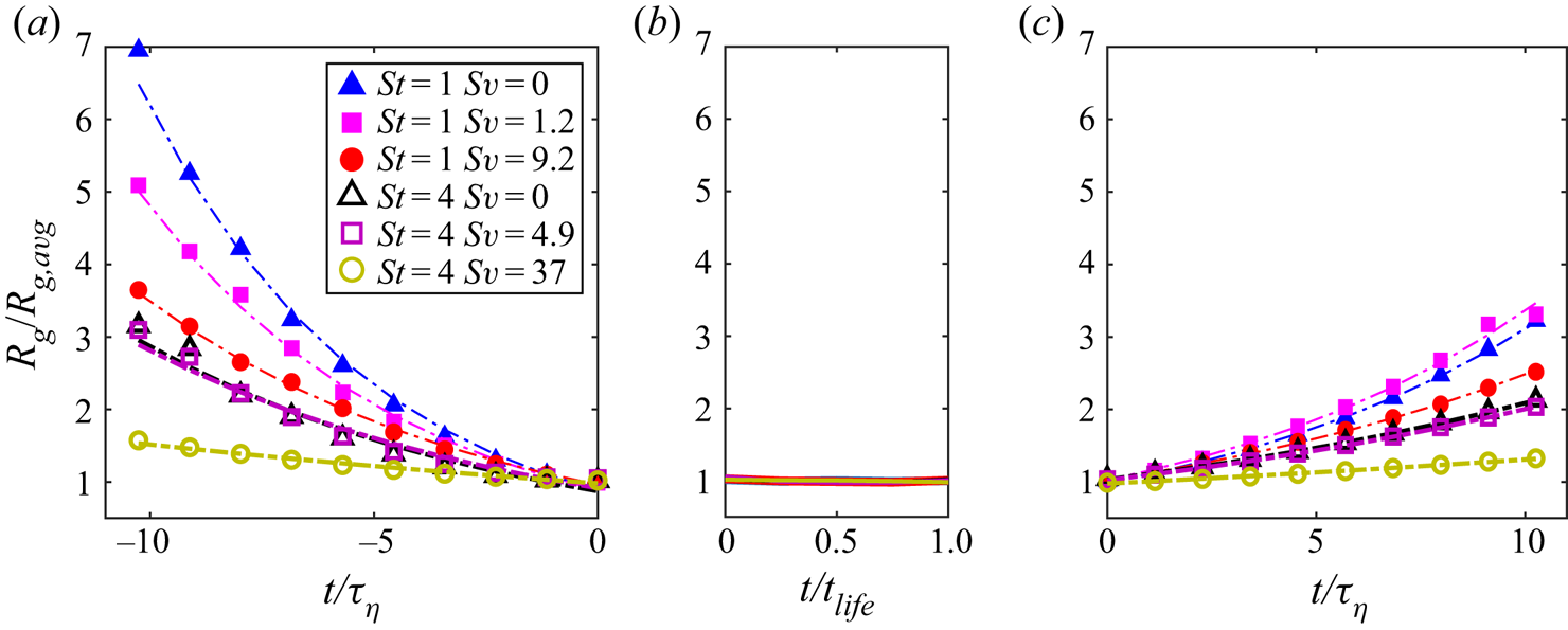
Figure 5. Evolution of the radius of gyration  $R_g$ of the particle clouds normalized by its average during
  $t_{life}$: (a) before birth, (b) during lifetime, and (c) after death, with lines indicating exponential best-fits. In panel (b), the temporal abscissa is normalized by the average cluster lifetime for each case.
3.4. The role of the turbulent activity
We finally turn our attention to the role played by turbulence in the clustering process. We use the local enstrophy  $\omega ^2$ to characterize small-scale turbulence activity (Carter & Coletti Reference Carter and Coletti2018). We interpolate
  $\omega ^2$ at the location of the particles belonging to the clouds considered in the previous subsection, and (similar to figure 5) we plot the ensemble-averaged values (normalized by their average during
  $t_{life}$ and denoted as
  $w^2_\textit{avg}$) before the birth (figure 6a), during the lifetime (figure 6b) and after the death of the clusters (figure 6c). The fluid enstrophy sampled by the cloud decays approximately linearly during the time before birth, grows at a somewhat faster rate after death, and remains relatively constant during the lifetime. The rate of change of the sampled enstrophy before birth and after death is much steeper for particles with St and Sv of order unity. Consider the case
  $St = 1, Sv = 1.2$. During lifetime, the clustered particles see an average enstrophy level around
  $24\,\%$ of the unconditional average in the computational domain. Approximately 10
 $\tau _\eta$ before birth (after death), they sample fluid with enstrophy around
  $75\,\%$ (
 $98\,\%$) of the unconditional average. This provides a strong indication of the mechanistic influence of small-scale turbulence activity on the formation, survival and destruction of inertial particle clusters: these are formed when a cloud of particles senses decreasing turbulence activity, persist while their environment is relatively quiet, and are disrupted by the next rise of local turbulence fluctuations. This behaviour appears to be most pronounced for the cases in which clustering is most intense, but is still present for particles with more inertia. We also note that using the local strain rate instead of the enstrophy leads to quantitatively analogous results (not shown). Therefore, the trends are not the consequence of the oversampling of low-enstrophy regions, but reveal a more fundamental tendency of the clusters to survive in times when the small-scale turbulence activity is weak.

Figure 6. Evolution of the enstrophy experienced by the particle clouds normalized by its average during  $t_{life}$: (a) before birth, (b) during lifetime and (c) after death. In panel (b), the temporal abscissa is normalized by the average cluster lifetime for each case.
4. Conclusions
We have carried out the first study of the temporal coherence of inertial particle clusters in turbulence. We have focused on a range of St (1 to 4) and Sv (0 to 37) leading to clusters of considerable size. The picture that emerges reveals several novel and unexpected aspects of particle-laden turbulence. The cluster lives have typical durations of a few Kolmogorov time scales, consistent with the idea that clustering is primarily driven by small-scale turbulence. Cluster lifetimes are strongly related to their size, i.e. large clusters tend to be long-lived, and vice versa. Accordingly, clusters formed by particles with more inertia (which are on average larger) last longer in time. Gravitational settling also increases lifetime because (for the present range of St) it reduces the influence of turbulent dispersion. Despite the strong link between size and lifetime, we remark that the former follows a power-law probability distribution (Monchaux et al. Reference Monchaux, Bourgoin and Cartellier2010; Baker et al. Reference Baker, Frankel, Mani and Coletti2017; Monchaux & Dejoan Reference Monchaux and Dejoan2017; Petersen et al. Reference Petersen, Baker and Coletti2019; Momenifar & Bragg Reference Momenifar and Bragg2020, among others), strongly suggestive of a self-similar process; while the latter follows an approximately exponential distribution, indicating a dominant time scale. Therefore, the relation between both quantities is non-trivial and its mathematical modelling requires further investigation.
By tracking individual particles before and after the formation of a cluster, we gain insight into its birth, survival and death. The most common scenario is the formation of small clusters from the coagulation of previously non-clustered particles, quickly followed by disintegration into parts mostly consisting of non-clustered particles. Large and long-lived clusters, on the other hand, are born most frequently by recombination of other similarly large clusters, and upon their death their components also recombine into new, large and long-lived clusters. This implies that, albeit rarely, the same particles may remain in a ‘clustered state’ for a time much longer than even the longest cluster lifetimes. This may have important consequences for the probability of particle–particle interaction. Particle clouds contract exponentially in time before giving birth to a cluster, and after its death they expand exponentially at a lower rate, consistently with the known asymmetry between forward-in-time and backward-in-time pair dispersion. This may also be related to the effective compressibility of the inertial particle field (Maxey Reference Maxey1987). However, as recently pointed out by Oujia, Matsuda & Schneider (Reference Oujia, Matsuda and Schneider2020), the relation between the local concentration and the sign of the particle velocity divergence is not trivial. In future studies, this point may be investigated coupling our approach to the method of Oujia et al. (Reference Oujia, Matsuda and Schneider2020), who tracked the rate of change of the Voronoï cell volumes. Both contraction rates and expansion rates generally decrease with increasing St and Sv.
For all considered cases, the cluster size is remarkably constant during its lifetime, and the particles experience anomalously low enstrophy and strain rate of the fluid turbulence. Specifically, the cluster formation happens during a phase in which the small-scale turbulence activity decays, and its disruption coincides with the end of such a quiet state. Thus, in contrast with the common view that clustering is associated with intense turbulence, the clusters need a relatively quiescent environment in order to survive for an extended amount of time. As weak turbulence fluctuations are associated with reduced inter-scale energy transfer rates (Carter & Coletti Reference Carter and Coletti2018), this points to a link between cluster formation and the turbulence cascade which deserves more attention. For similar reasons, further research is warranted to investigate higher Reynolds numbers for which intermittency is more intense, as this may have direct impact on the cluster lifetime. Moreover, the large-scale spatial organization of small-scale turbulence activity (also dependent on the Reynolds numbers) is likely to impact the life cycle of the clusters, which are shown to form and evolve over inertial-range scales.
In the future, a more articulated view of the merging and splitting of clusters can be gained by the applications of graph theory, which has been successfully used to investigate the evolution of clusters of vortices in wall turbulence (Lozano-Durán & Jiménez Reference Lozano-Durán and Jiménez2014). Also, light bubbles are known to produce even more concentrated and long-lived clusters (Tagawa et al. Reference Tagawa, Mercado, Prakash, Calzavarini, Sun and Lohse2012; Mathai, Lohse & Sun Reference Mathai, Lohse and Sun2020), and, therefore, the present methodology is expected to provide similar insight into bubble-laden turbulence. In general, the approach can be applied to any system of clustering elements that can be tracked in a Lagrangian framework.
Acknowledgements
This simulation work was performed using HPC resources from GENCI-CINES. We would like to acknowledge the Minnesota Supercomputing Institute (MSI) at the University of Minnesota for providing computational resources for result analysis. We are thankful to L. J. Baker for her contribution in the implementation of the Voronoï tessellation code.
Declaration of interests
The authors report no conflict of interest.


