


1. Introduction
Surface reactions such as adsorption and desorption are very common in reactive solute transport problems in many applications of chemistry, biology, hydraulics, etc. For example, in gas chromatography, the function of the stationary phase in the coated column is related to the sorption process (Giddings & Eyring Reference Giddings and Eyring1955; Golay Reference Golay1958; Clifford et al. Reference Clifford, Gray, Mason and Waddicor1982; Hlushkou et al. Reference Hlushkou, Gritti, Guiochon, Seidel-Morgenstern and Tallarek2014). In membrane science, the adsorption–desorption process of surfactants can change the rheological parameters of the interfaces (Bleys & Joos Reference Bleys and Joos1985; Langevin Reference Langevin2014). The adsorption and desorption kinetics are also widely observed in molecule–surface interactions, including protein binding and release, synaptic communication, membrane permeability and heterogeneous catalysis (Fang, Satulovsky & Szleifer Reference Fang, Satulovsky and Szleifer2005; Andrews Reference Andrews2009; Deng et al. Reference Deng, Noel, Elkashlan, Nallanathan and Cheung2015; Lotter, Ahmadzadeh & Schober Reference Lotter, Ahmadzadeh and Schober2021). For contaminant and sediment transport in natural streams, the transient storage model with sorptive exchange is widely used to characterise the transport processes affected by the dead zones or places where the flow speed is slow, and the hyporheic exchange with the stream bed (Sayre Reference Sayre1967; Valentine & Wood Reference Valentine and Wood1977; Nordin & Troutman Reference Nordin and Troutman1980; Ng & Yip Reference Ng and Yip2001; Sandoval et al. Reference Sandoval, Mignot, Mao, Pastén, Bolster and Escauriaza2019; Wang & Cirpka Reference Wang and Cirpka2021).
The term reversible describes that the adsorbed solute mass from the bulk to the boundary surface can be released back to the flow through the desorption process (Goodrich Reference Goodrich1954; Boddington & Clifford Reference Boddington and Clifford1983; Purnama Reference Purnama1988a), which is a generalisation of the irreversible pure-adsorption (wall absorption) process (Gupta & Gupta Reference Gupta and Gupta1972; Pancharatnam & Homsy Reference Pancharatnam and Homsy1972; Mauri Reference Mauri1991; Sadeghi et al. Reference Sadeghi, Saidi, Moosavi and Sadeghi2020; Wang et al. Reference Wang, Jiang, Chen and Tao2022). Therefore, this reversible kinetic sorption is generally more appropriate for applications in practice, whereas the corresponding transport processes are more complicated. Several models have been proposed for the reversible adsorption phenomenon (Purnama Reference Purnama1988a). In the context of chromatography, a wall condition with the time derivative of concentration for the absorbed solute was proposed in the pioneering work of Golay (Reference Golay1958). Later, Aris (Reference Aris1959) and Khan (Reference Khan1962) used a two-zone (or two-phase) model for the transport in the bulk and the retentive layer (the thickness of which is finite), with an interface condition describing the reversible exchange between zones (phases), which was then extended by Horn (Reference Horn1971) and Davidson & Schroter (Reference Davidson and Schroter1983). Boddington & Clifford (Reference Boddington and Clifford1983) proposed a more general type of boundary condition based on Golay's one-zone model for reversible adsorption–desorption, including effects of the irreversible adsorption in the infinitely thin retentive layer. The transport equations for the concentration distribution in the bulk and that on the surface are thus coupled. This form of wall condition is simple and later widely used in applications of other fields such as biology (Lotter et al. Reference Lotter, Ahmadzadeh and Schober2021) and hydraulics (Nordin & Troutman Reference Nordin and Troutman1980). In practice, a first-order linear reaction model is most popular for the adsorption–desorption process (Balakotaiah & Chang Reference Balakotaiah and Chang1995; van Duijn et al. Reference van Duijn, Mikelić, Pop and Rosier2008; Paul & Mazumder Reference Paul and Mazumder2011; Roy, Saha & Debnath Reference Roy, Saha and Debnath2020). However, an analytical study on such a basic linear reactive transport problem is still challenging and thus of great interest.
Taylor dispersion (Taylor Reference Taylor1953, Reference Taylor1954) is a fundamental mechanism highlighting the effective longitudinal diffusion of solute cloud at the long-time asymptotic transport regime, as contributed by the combined action of transverse diffusion and flow shear. Such an understanding provides a powerful tool in the analysis of the macro-transport processes in confined flows (Taghizadeh, Valdés-Parada & Wood Reference Taghizadeh, Valdés-Parada and Wood2020; Chu et al. Reference Chu, Garoff, Tilton and Khair2021). For the reactive transport with adsorption–desorption, a central problem under investigation is how the reversible adsorption will influence the macro-transport characteristics, e.g. the transverse concentration distribution at the equilibrium state, the effective drift and the effective diffusion coefficient (Taylor dispersivity). Most studies focused on the long-time asymptotic process of solute dispersion and there are several popular theoretical methods to this end. The homogenisation method with perturbation technique (Purnama Reference Purnama1988a; Ng & Yip Reference Ng and Yip2001; Ng Reference Ng2006; Allaire, Mikelić & Piatnitski Reference Allaire, Mikelić and Piatnitski2010; Paul & Mazumder Reference Paul and Mazumder2011; Barik & Dalal Reference Barik and Dalal2022), and the centre manifold method (Mercer & Roberts Reference Mercer and Roberts1994), for example, are powerful and easy-to-apply to the treatment of transport processes with nonlinear reactions (Balakotaiah & Chang Reference Balakotaiah and Chang1995, Reference Balakotaiah and Chang2003; Barik & Dalal Reference Barik and Dalal2017). Alternatively, some other methods including the method of concentration moments by Aris (Reference Aris1956) and the generalised dispersion model by Gill (Reference Gill1967), are in nature capable of addressing the initial transient dispersion of solute immediately after its release. In practice, this was mainly done for the transport processes without reactions, or with simple irreversible adsorption on the tube wall. For more complicated reactions such as the processes with reversible adsorption and desorption, these two methods have mainly been applied to obtain dispersion characteristics for the Taylor dispersion regime (Boddington & Clifford Reference Boddington and Clifford1983; Clifford Reference Clifford1989; Valocchi Reference Valocchi1989; Levesque et al. Reference Levesque, Bénichou, Voituriez and Rotenberg2012; Berezhkovskii & Skvortsov Reference Berezhkovskii and Skvortsov2013; Alexandre, Guérin & Dean Reference Alexandre, Guérin and Dean2021), due to difficulties brought by the coupling of the adsorption and desorption, and the complexity in mathematics of applying these methods (Ng & Rudraiah Reference Ng and Rudraiah2008). In contrast to the above-mentioned theoretical analysis, there are considerable numerical studies using tools such as the finite-difference method (Lau & Ng Reference Lau and Ng2007; Ng & Rudraiah Reference Ng and Rudraiah2008; Mazumder & Paul Reference Mazumder and Paul2012), lattice Boltzmann method (Vanson et al. Reference Vanson, Coudert, Rotenberg, Levesque, Tardivat, Klotz and Boutin2015; Zhang, Hesse & Wang Reference Zhang, Hesse and Wang2017; Zaafouri et al. Reference Zaafouri, Batôt, Nieto-Draghi, Rotenberg, Bauer and Coasne2021) and Brownian dynamics simulation (Andrews Reference Andrews2009; Deng et al. Reference Deng, Noel, Elkashlan, Nallanathan and Cheung2015). Recently, Debnath et al. (Reference Debnath, Saha, Mazumder and Roy2019) and Debnath, Ghoshal & Kumar (Reference Debnath, Ghoshal and Kumar2021) have numerically solved the moment equations and analysed the transient dispersion evolution for various flow conditions.
Aiming at analytically studying the transient solute transport before approaching the Taylor dispersion regime, Zhang et al. (Reference Zhang, Hesse and Wang2017) investigated the temporal evolution of the moments and corresponding dispersion characteristics under the reversible adsorption, to understand the non-equilibrium evolution of the solute concentration distribution. To solve the coupled equations for moments of bulk and surface concentration, they applied the Laplace transform with respect to the time variable. The adsorption–desorption boundary condition turns out to be a Robin boundary condition (the third type) for the transport equation in the frequency domain (Zhang et al. Reference Zhang, Hesse and Wang2017, equation (3.8)). They found that when the initial distribution is transversely uniform, the zeroth-order moment decays exponentially to reach the equilibrium state. The drift of solute will first increase and then decrease at large times, whereas the evolution of dispersivity is much more complicated. It is found that reversible adsorption can reduce both the drift and dispersivity (Zhang, Hesse & Wang Reference Zhang, Hesse and Wang2017, Reference Zhang, Hesse and Wang2019), due to the desorption of the retentive solute from the wall to the slow-flow-speed region. The time scale of the transition to the Taylor dispersion regime increase with the ratio of adsorption to desorption rates. Hence, the method of Laplace transform has been used a lot in analysing the evolution of the concentration distribution. And many studies (Agmon Reference Agmon1984; Kim & Shin Reference Kim and Shin1999; Deng et al. Reference Deng, Noel, Elkashlan, Nallanathan and Cheung2015; Grebenkov Reference Grebenkov2019; Lotter, Ahmadzadeh & Schober Reference Lotter, Ahmadzadeh and Schober2020) have paid more attention to the simpler one-dimensional transport process, with the governing equation the same as that for the zeroth-order moment.
Although the application of the Laplace transform method was proven successful in theoretically capturing the transient evolution of concentration moments, the coupled adsorption–desorption of the solute mass between the bulk and the boundary wall has greatly increased the complexity of the solution procedure. Specifically, the inverse Laplace transform is the most difficult part of the analysis. Although it is relatively easy to perform the Laplace transform with respect to the time and obtain the expression of moments in the frequency domain ( $s$-plane), most likely one cannot find corresponding inverse formulae tabulated in the table of Laplace transform, and this last step is usually done by performing numerical inversions (Mehmani & Balhoff Reference Mehmani and Balhoff2014; Deng et al. Reference Deng, Noel, Elkashlan, Nallanathan and Cheung2015). Another means is to apply the residue theorem as done by Zhang et al. (Reference Zhang, Hesse and Wang2017, § 3.2) to calculate the inverse integral (see also the pure-diffusion case discussed by Lotter et al. Reference Lotter, Ahmadzadeh and Schober2020, Reference Lotter, Ahmadzadeh and Schober2021): they found that the first two-order moments in the frequency domain only have singularities up to the third order. They applied L'Hospital's rule for the limiting case of the formula leading to a sequence of residues, and eventually obtained the explicit form of the solutions in the time domain. It is noted that even with the residue theorem, the procedure and results obtained are still very complicated and inconvenient. For example, the coefficients in the solutions are so tedious that it takes almost five pages to present the expressions, as shown in the supplementary material of Zhang et al. (Reference Zhang, Hesse and Wang2017). Therefore, it is not feasible to widely apply this solution procedure using the Laplace transform method for problems in different fields.
This work is to provide a much simpler analytical procedure for concentration moments of the reactive transport process with boundary adsorption and desorption. Instead of using the Laplace transform, we directly resort to the classic method of separation of variables (Aris Reference Aris1956), which has been widely used for dispersion problems with pure adsorption (Lupa & Dranoff Reference Lupa and Dranoff1966; Sankarasubramanian & Gill Reference Sankarasubramanian and Gill1973; Smith Reference Smith1983; Barton Reference Barton1984; Mikelić, Devigne & van Duijn Reference Mikelić, Devigne and van Duijn2006), and to solve the two-zone model with phase exchange (Horn Reference Horn1971; Davidson & Schroter Reference Davidson and Schroter1983; Purnama Reference Purnama1988b; Li et al. Reference Li, Zhang, Qian, Huang, Wang and Zhao2021). Specifically, Barton (Reference Barton1983) has established a general framework for the expressions of moments based on the eigenfunction expansion of Sturm–Liouville theory (in which the eigenvalues and eigenfunctions need to be solved first), which was later extended to handle the case with irreversible wall adsorption (Barton Reference Barton1984). It remains unclear how this framework can be applied for the more general case of solute transport with reversible adsorption–desorption processes. The novelty of this work is thus to tackle this kind of boundary condition under Barton's general framework. The key is to solve the eigenvalue problem for the coupled concentration distributions in the bulk and on the tube wall surface. Then one can readily obtain the analytical solution for the concentration moments: simply replacing the eigenvalues and eigenfunctions in Barton's expressions with those determined for the adsorption–desorption boundary condition. As the structure of the solution is clearly revealed by the eigenfunctions, the newly developed solution procedure is more intuitive, adaptive and convenient than the previously used Laplace transform method.
Note that characterising the non-Gaussian concentration distributions for the initial transient transport respectively for the bulk flow and the sorptive wall is of fundamental importance. Skewness is a commonly used measure for the longitudinal asymmetry of these distributions. Many studies have discussed the skewness through numerical simulations or experiments, and it was found that the skewness of the concentration distribution in the sorptive layer is quite large (Nordin & Troutman Reference Nordin and Troutman1980; Fornstedt, Zhong & Guiochon Reference Fornstedt, Zhong and Guiochon1996; Boano et al. Reference Boano, Packman, Cortis, Revelli and Ridolfi2007; Bishop et al. Reference Bishop, Misiura, Moringo and Landes2020). Probably due to the complexity of the analytical method, Zhang et al. (Reference Zhang, Hesse and Wang2017) only discussed the zeroth-order moment, the drift and the dispersivity, namely moments up to the second order in their paper. With the progress of our simpler method, it is now possible to further analyse the temporal evolution of higher-order statistics such as skewness and kurtosis. As discussed previously, Gill's generalised dispersion model is one of the analytical tools that can be used to analyse the transient dispersion characteristics (Ng & Rudraiah Reference Ng and Rudraiah2008; Mazumder & Paul Reference Mazumder and Paul2012), which on the other hand also provides a means of directly constructing the analytical solution for the solute concentration distribution based on higher-order concentration moments. Thus, in this paper, we also exploit and extend Gill's generalised dispersion model by increasing the expansion order to reflect the non-Gaussian effects including the skewness, and using the transient transport coefficients at higher orders to obtain concentration distributions for the bulk and the wall surface, respectively.
The rest of this paper is structured as follows. The transport problem in a tube flow with adsorption–desorption boundary condition is formulated in § 2. For simplicity, we focus on the axisymmetric case. Then, we introduce the definition of longitudinal moments and dispersion characteristics in § 3, respectively for four concentration distributions: concentration in the bulk, concentration on the surface, as well as the transverse- and the total-average concentration. The eigenvalue problem is constructed in § 4 and concentration moments are solved by the orthogonal expansion based on the framework of Barton (Reference Barton1983, Reference Barton1984), the analytical solutions of which are verified by performing the Brownian dynamics simulation. We then apply Gill's generalised dispersion model in § 5 to calculate the concentration distributions. In § 6, the dispersion characteristics: the zeroth-order moment, the drift, the apparent dispersivity and the skewness are analysed for the Poiseuille flow. We specifically focus on the differences between the transverse- and the total-average characteristics, and the effects of the initial conditions. Finally, § 7 concludes.
2. Formulation
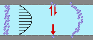
As sketched in figure 1, we consider reactive solute transport in a tube with irreversible wall adsorption, reversible wall adsorption and desorption. There are two concentration distributions in this problem considering the adsorption–desorption: the bulk concentration ( $C(x,r,t)$) and the surface concentration at the wall (
 $C_s(x,t)$). Following Ng & Rudraiah (Reference Ng and Rudraiah2008), for simplicity, we focus on the axisymmetric transport problem or the concentration profile averaged over the azimuthal angle.

Figure 1. Sketch of solute particles dispersing in shear flow with adsorption and desorption on the tube wall.
This reactive transport problem can be written in the dimensionless form as
 $$\begin{gather} \frac{\partial C}{\partial t} + Pe \,u (r) \frac{\partial C}{\partial x} = \frac{\partial^2 C}{\partial x^2} + \frac{1}{r} \frac{\partial}{\partial r} \left(r \frac{\partial C}{\partial r} \right), \quad 0< r<1, -\infty < x<\infty, \end{gather}$$
 $$\begin{gather}- \left. \frac{\partial C}{\partial r} \right|_{r = 1} - k_{ia} \left. C \right|_{r = 1} = \frac{\partial C_s}{\partial t} = k_a C |_{r = 1} - k_d C_s, \end{gather}$$
 $$\begin{gather}\left. \frac{\partial C}{\partial r} \right|_{r = 0}\quad \text{is finite}, \end{gather}$$
 $$\begin{gather}C |_{t = 0} = \delta (x) C^{{Int}}(r), \end{gather}$$
 $$\begin{gather}C_s |_{t = 0} = \delta (x) C^{{Int}}_s, \end{gather}$$
where the following dimensionless variables and parameters (the superscript  $\ast$ denotes dimensional variables or the dimensional counterpart) are considered:
 \begin{equation} \left. \begin{gathered} t = \frac{t^{{\ast}}}{R^{{\ast} 2} / D^{{\ast}}}, \quad x = \frac{x^{{\ast}}}{R^{{\ast}}}, \quad r = \frac{r^{{\ast}}}{R^{{\ast}}}, \quad C = \frac{C^{{\ast}}}{m^{{\ast}}/({\rm \pi} R^{{\ast} 3})}, \quad C_s = \frac{C_s^{{\ast}}}{m^{{\ast}}/({\rm \pi} R^{{\ast} 2})},\\ u = \frac{u^{{\ast}}}{\bar{u}^{{\ast}}},\quad Pe = \frac{\bar{u}^{{\ast}} R^{{\ast}}}{D^{{\ast}}}, \quad k_{ia} = \frac{k_{ia}^{{\ast}}}{D^{{\ast}} / R^{{\ast}}},\quad k_a = \frac{k_a^{{\ast}}}{D^{{\ast}} / R^{{\ast}}},\quad k_d = \frac{k_d^{{\ast}}}{D^{{\ast}} / R^{{\ast} 2}} , \end{gathered}\right\} \end{equation}
and  $t^{\ast }$ is the time,
  $x^{\ast }$ is the longitudinal coordinate,
  $r^{\ast }$ is the radial coordinate,
  $R^{\ast }$ is the radius of the tube,
  $D^{\ast }$ is the diffusion coefficient,
  $m^{\ast }$ is the total mass of the released solute,
  $u^{\ast }$ is the velocity profile and
  $\bar {u}^{\ast }$ is the mean flow speed. The Péclet number
  $Pe$ quantifies the relative importance of advection and effective diffusion.
  $k_{ia}^{\ast }$ represents the irreversible adsorption rate of the surface. Accordingly,
  $k_a^{\ast }$ defines the reversible adsorption rate of the surface and
  $k_d^{\ast }$ is the reversible desorption rate.
For the initial conditions (2.1d) and (2.1e), the solute is assumed to be instantaneously released in a cross-section of the tube. The initial radial distribution ( $C^{{Int}}(r)$ in the bulk and
  $C^{{Int}}_s$ on the surface) is axisymmetric.
Note that the adsorption–desorption boundary condition (2.1b), as reported by Boddington & Clifford (Reference Boddington and Clifford1983, equation (1.6)), assumes that the adsorbed solute from the bulk to the wall can be ‘released’ back to the bulk by desorption, which is known as the reversible effect. It also includes the process of irreversible adsorption, as represented by  $k_{i a}$. Adopting a linear kinetic model, both the adsorption and desorption are assumed to be first-order reactions. Obviously, when
  $k_d=0$, the adsorption is irreversible (Gupta & Gupta Reference Gupta and Gupta1972). Under the condition of
  $k_{ia}=k_a=0$, (2.1b) represents a pure desorption; together with
  $k_d=0$, it is simplified into the non-penetration condition (i.e. zero flux across the tube wall) (Taylor Reference Taylor1953). These simplified cases are relatively easy to explore analytically because
  $C$ and
  $C_s$ are decoupled. Moreover, for
  $k_{ia}=0$,
  $k_a\rightarrow \infty$ and
  $k_d \rightarrow \infty$ with a fixed ratio (i.e. the partition number
  $k=k_a/k_d$), the surface sorption will soon lead to a local equilibrium, i.e.
  $k_a C|_{r = 1} = C_s k_d$ (Zhang et al. Reference Zhang, Hesse and Wang2017). Consequently, the linear kinetic model (2.1b) turns into the primitive model (Golay Reference Golay1958), as pointed out by Boddington & Clifford (Reference Boddington and Clifford1983, equation (8.10)). To some extent, the two-zone model (Aris Reference Aris1959) can be viewed as an extension of (2.1b) with an exchangeable layer of finite width, although the mathematical formulations of the two transport problems are different. Take the mean concentration over the finite static surface layer as an overall
  $C_s$, then the two-zone model can be approximated by a one-zone problem given the boundary condition (2.1b) (Khan Reference Khan1962; Horn Reference Horn1971). A further simplification is that the transport in the bulk can also be modelled by a one-dimensional effective equation with an exchange term
  $C_s$, which is widely used in chemical and environmental applications (Nordin & Troutman Reference Nordin and Troutman1980; Balakotaiah & Chang Reference Balakotaiah and Chang1995; Kim et al. Reference Kim, Seo, Kwon, Jung and Choi2021).
3. Moments of concentration distribution
3.1. Definition of moments
Instead of solving the transport problem (2.1) directly, we resort to the classic method of moments (Aris Reference Aris1956) and analyse the basic characterises of concentration distribution, i.e. the first three-order moments related to the total amount of solute mass, the averaged moving speed of solute cloud (drift), the effective diffusion (apparent dispersivity) and the longitudinal asymmetry of the solute concentration distribution (skewness).
The longitudinal moments of the concentration distributions in the bulk and on the wall surface are defined as (Aris Reference Aris1956)
 \begin{equation} M_n = \int^{\infty}_{- \infty} x^n C \, \mathrm{d}\kern0.06em x, \quad M_{s n} = \int^{\infty}_{- \infty} x^n C_s \, \mathrm{d}\kern0.06em x. \quad n = 0, 1, \ldots. \end{equation}
The moments of the cross-sectional-average concentration (hereafter referred to as the transverse-average concentration)
 \begin{equation} \bar{C} = \int^1_0 2 r C \, \mathrm{d} r \end{equation}
is also considered. We use the overbar to denote variables related to the transverse-average concentration, and
 \begin{equation} \bar{M}_n = \int^{\infty}_{-\infty} x^n \bar{C} \, \mathrm{d}\kern0.06em x, \quad n = 0, 1, \ldots \end{equation}
is the transverse-average moments. We also consider the total-average concentration (total solute mass during the reversible transport process), i.e.
 \begin{equation} \bar{\bar{C}} = \int^1_0 2 r C \, \mathrm{d} r + 2 C_s =\bar{C}+2 C_s, \end{equation}
where the double overbar denotes the average over the bulk (mobile phase) and the wall surface (stationary phase adsorbed on the surface). Thus, total-average moments are
 \begin{equation} \bar{\bar{M}}_n = \int^{\infty}_{- \infty} x^n \bar{\bar{C}} \, \mathrm{d}\kern0.06em x = \bar{M}_n + 2 M_{s n} \quad n = 0, 1, \ldots. \end{equation}
Note that  $\bar {M}_0$ represents the amount of solute in the bulk,
  $\bar {M}_{s 0}$ is the amount on the surface, whereas
  $\bar {\bar {M}}_0$ represents the total amount of reversible solute in the tube. Some solute will be permanently removed from the reactive transport process by the irreversible adsorption.
3.2. Basic dispersion characteristics
Now we have four concentration distributions:  $C$ in the bulk,
  $C_s$ on the surface, the transverse-average
  $\bar {C}$ and the total-average
  $\bar {\bar {C}}$. Therefore, for each distribution, we can analyse its basic dispersion characteristics by the associated moments, such as the drift (the first-order moment), apparent dispersivity (second order) and the skewness (third order). In the following, we take the transverse-average distribution as an example.
First, the transverse-average drift  $\bar {U}_a$ and apparent dispersivity
  $\bar {D}_a$ are defined as the time derivatives of the expected value (
 $\bar {\mu }$) and the variance (
 $\bar {\sigma }^2$), respectively (Dentz & Carrera Reference Dentz and Carrera2007). We normalise the transverse-average concentration distribution as
  $\bar {P}= \bar {C} /\bar {M}_0$, which is a well-defined probability distribution. Then,
 $$\begin{gather} \bar{U}_a (t) = \frac{\mathrm{d} \bar{\mu}}{\mathrm{d} t} =\frac{\mathrm{d} \bar{P}_1}{\mathrm{d} t} = \frac{\mathrm{d}}{\mathrm{d} t} \left( \frac{\bar{M}_1}{\bar{M}_0} \right), \end{gather}$$
 $$\begin{gather}\bar{D}_a (t) = \frac{1}{2} \frac{\mathrm{d} \bar{\sigma}^2}{\mathrm{d} t} = \frac{1}{2} \frac{\mathrm{d}}{\mathrm{d} t} \left( \bar{P}_2 - \bar{P}_1^2 \right) = \frac{1}{2} \frac{\mathrm{d}}{\mathrm{d} t} \left[ \frac{\bar{M}_2}{\bar{M}_0} - \left( \frac{\bar{M}_1}{\bar{M}_0} \right)^2 \right], \end{gather}$$
where  $\bar {P}_1 = {\bar {M}_1}/{\bar {M}_0}$ and
  $\bar {P}_2 = {\bar {M}_2}/{\bar {M}_0}$ are the normalised moments. Similarly, we can define
  $U_a$ and
  $D_a$ in the bulk,
  $U_{a s}$ and
  $D_{a s}$ on the surface and the total-average drift
  $\bar {\bar {U}}_a$ and the dispersivity
  $\bar {\bar {D}}_a$.
The long-time asymptotic values of drift and dispersivity are required as the coefficients in the Taylor dispersion model (Taylor Reference Taylor1953). Namely,  $\lim _{t \rightarrow \infty } \bar {D}_a (t) = D_e$, where
  $D_e$ is the Taylor dispersivity. Note that we use the term ‘apparent’ dispersivity (or apparent dispersion coefficient, with subscript ‘
 $a$’) from previous work (Dagan Reference Dagan1988; Dentz & Carrera Reference Dentz and Carrera2007) to avoid ambiguity with Taylor dispersivity (with subscript ‘
 $e$’). Hereafter, the apparent dispersivity is referred to as dispersivity for brevity.
Furthermore, the skewness is also of interest because it can reflect the longitudinal asymmetry of the distribution and the deviation from Gaussian distribution. It is defined as
 \begin{equation} \overline{\mathit{Sk}} = \frac{\bar{\kappa}_3}{\bar{\sigma}^3} = \frac{\bar{P}_3 - 3 \bar{P}_2 \bar{P}_1 + 2 \bar{P}_1^3}{\bar{\sigma}^3}, \end{equation}
where  $\bar {\kappa }_3$ is the third-order cumulant of the normalised distribution and
  $\bar {P}_3$ is the third-order normalised moment (
 $\bar {P}_3 = {\bar {M}_3}/{\bar {M}_0}$). We can also define the skewness for the other three distributions after normalisation. Higher-order moments can provide additional information regarding the solute concentration distribution but it becomes more and more challenging to analytically obtain their explicit expressions. Thus, we only give a brief discussion on the kurtosis in Appendix B and the other higher-order statistics are not considered in this paper.
4. Solutions of moments
Solving the moments is the first step to obtain the above-discussed basic dispersion characteristics and to further construct the concentration distributions. We can simply use the generic solution expressions of moments (with eigenvalues and eigenfunctions to be determined) given by Barton (Reference Barton1983, Reference Barton1984). Hence, the key is to solve the corresponding eigenvalue problem for the coupled concentration moments in the bulk and on the surface. The construction of the eigenvalue problem under conditions of the coupled adsorption–desorption processes is similar to that for the two-zone model (Aris Reference Aris1959). Specifically, we follow procedures as listed below. First, we obtain the governing equation of moments. We denote the elements in a vector form to recast the equation in the same form as that presented in Barton's framework. Then the eigenvalue problem is extracted and solved. Finally, we substitute the solved eigenvalues and eigenfunctions into Barton's expressions for the solution.
4.1. Governing equation of moments
Integrate the governing equation (2.1a) and boundary conditions (2.1b) and (2.1c) according to the definition of moments (3.1), then we have
 $$\begin{gather} \frac{\partial M_n}{\partial t} - n \,Pe (r) M_{n - 1} = n (n - 1) M_{n - 2} +\frac{1}{r} \frac{\partial}{\partial r} \left( r \frac{\partial M_n}{\partial r} \right) , \quad 0< r<1, \end{gather}$$
 $$\begin{gather}- \left. \frac{\partial M_n}{\partial r} \right|_{r = 1} - k_{i a} \left. M_n \right|_{r=1} = \frac{\partial M_{s n}}{\partial t}= k_a M_n |_{r = 1} - k_d M_{s n} \end{gather}$$
 $$\begin{gather}\left. \frac{\partial M_n}{\partial r} \right|_{r = 0} \quad \text{is finite}, \end{gather}$$
for  $n=0,1,\ldots$ and
  $M_{-1}=M_{-2}=0$. Equation (4.1b) is the wall condition with adsorption and desorption. The corresponding initial conditions for (2.1d) and (2.1e) are
 \begin{equation} M_n |_{t = 0} = \left\{\begin{array}{ll} C^{{Int}}(r), & n = 0,\\ 0, & n = 1, 2, \ldots, \end{array}\right. \quad M_{s n} |_{t = 0} = \left\{\begin{array}{ll} C^{{Int}}_s, & n = 0,\\ 0, & n = 1, 2, \ldots. \end{array}\right. \end{equation}
Note that due to the adsorption–desorption boundary condition (4.1b), the moments  $M_n$ and surface moment
  $M_{s n}$ are coupled.
4.2. Recast moment equations using matrix notation
We use a column vector  $\boldsymbol {c}$ to denote the two components (
 $C$ in the bulk and
  $C_s$ on the surface) of the whole concentration:
  $\boldsymbol {c}=(C, C_s)^{\mathrm {T}}$, where the superscript
  $\mathrm {T}$ denotes the transpose. Accordingly, for moments,
  $\boldsymbol {m}_n=(M_n, M_{s n})^{\mathrm {T}}$,
  $n=0,1,\ldots$.
Next, we introduce a linear operator  $\mathcal {L}$ with respect to
  $r$ for the governing equations (4.1a) and (4.1b):
 \begin{equation} \mathcal{L} ({\boldsymbol{f}}) = \begin{pmatrix} \dfrac{1}{r} \dfrac{\partial}{\partial r} \left( r \dfrac{\partial f}{\partial r} \right) \\ k_a f |_{r = 1} - k_d f_s \end{pmatrix}, \end{equation}
where  ${\boldsymbol {f}}$ is arbitrary concentration vector function
  ${\boldsymbol {f}}= (f, f_s)^{\mathrm {T}}$. The element-wise product
  $\odot$ (Hadamard product) is adopted, for any
  $\boldsymbol {f}$ and
  $\boldsymbol {g}$,
 \begin{equation} {\boldsymbol{f}} \odot {\boldsymbol{g}}= \begin{pmatrix} f\\ f_s \end{pmatrix} \odot \begin{pmatrix} g\\ g_s \end{pmatrix} = \begin{pmatrix} f g\\ f_s g_s \end{pmatrix}. \end{equation}
Then (4.1a) and (4.1b) can be recast as
 \begin{equation} \frac{\partial {\boldsymbol{m}}_n}{\partial t} =\mathcal{L}({\boldsymbol{m}}_n) + n \,Pe\, {\boldsymbol{u}} \odot {\boldsymbol{m}}_{n - 1} + n (n - 1) {\boldsymbol{d}} \odot {\boldsymbol{m}}_{n - 2}, \end{equation}
for  $n=0,1,\ldots$ and
  $\boldsymbol {m}_{-1}=\boldsymbol {m}_{-2}=0$ (auxiliary terms). Note that we construct the velocity vector as
  $\boldsymbol {u}=(u(r), 0)^{\mathrm {T}}$ and the diffusion coefficient vector as
  $\boldsymbol {d}=(1, 0)^{\mathrm {T}}$, because there is no advection and diffusion on the sorptive surface. Now, (4.5) is in the same form as the classic (one-zone) moment equation in the work of Barton (Reference Barton1983, Reference Barton1984).
4.3. Eigenvalue problem
The eigenvalue problem is constructed as that of the two- or multi-zone problem (Davidson & Schroter Reference Davidson and Schroter1983; Shankar & Lenhoff Reference Shankar and Lenhoff1991; Jiang & Chen Reference Jiang and Chen2019), and can be solved using the method of separation of variables for (4.5). It is straightforward to find
 \begin{equation} \mathcal{L} ({\boldsymbol{f}}) ={-}\lambda {\boldsymbol{f}}, \end{equation}
where  $\lambda$ is the eigenvalue and
  ${\boldsymbol {f}}=(f, f_s)^{\mathrm {T}}$ is the corresponding eigenfunction. The last two terms on the right-hand side of (4.5) are source terms. With boundary conditions (4.1b) and (4.1c), the whole eigenvalue problem in the form of components is
 $$\begin{gather} \frac{1}{r} \frac{\partial}{\partial r} \left( r \frac{\partial f}{\partial r} \right) ={-}\lambda f, \end{gather}$$
 $$\begin{gather}k_a f |_{r = 1} - k_d f_s ={-}\lambda f_s, \end{gather}$$
 $$\begin{gather}- \left. \frac{\partial f}{\partial r} \right|_{r = 1} - k_{i a} \left. f \right|_{r = 1} = k_a f |_{r= 1} - k_d f_s, \end{gather}$$
 $$\begin{gather}\left. \frac{\partial f}{\partial r} \right|_{r = 0} \quad \text{is finite}. \end{gather}$$
 This problem can be solved easily. For physical reasoning, we expect  $\lambda \geqslant 0$ to exclude the exponential growth, thus the solution for (4.7a) with (4.7d) is
 \begin{equation} f (r) = a \mathrm{J}_0 ( \sqrt{\lambda} r ), \end{equation}
where  $\mathrm {J}_0$ is the zeroth-order Bessel function of the first kind and
  $a$ is an undetermined coefficient. Based on (4.7b) and (4.7c), we have
 \begin{equation} f_s = a \frac{k_a}{k_d - \lambda} \mathrm{J}_0 ( \sqrt{\lambda}), \end{equation}
and the transcendental equation for  $\lambda$
 \begin{equation} \frac{\mathrm{J}_1 ( \sqrt{\lambda})}{\mathrm{J}_0 ( \sqrt{\lambda})} = \frac{k_{i a}}{\sqrt{\lambda}} - \frac{k_a \sqrt{\lambda}}{k_d - \lambda}, \end{equation}
which results in a sequence of eigenvalues,  $\{\lambda _i \}_0^{\infty }$, guaranteeing the completeness of the basis of eigenfunctions. We denote the corresponding sequence of eigenfunctions as
  $\{ \boldsymbol {e}_i \}_0^{\infty }$, and
 \begin{equation} {\boldsymbol{e}}_i = \begin{pmatrix} e_i (r)\\ e_{s i} \end{pmatrix} = a \begin{pmatrix} \mathrm{J}_0 ( \sqrt{\lambda} r )\\ \dfrac{k_a }{k_d - \lambda} \mathrm{J}_0( \sqrt{\lambda}) \end{pmatrix}, \quad i=0,1,\ldots, \end{equation}
where the constant  $a$ is a normalisation factor.
As shown in figure 2, the roots of the transcendental equation (4.10) can be found by the intersections of two curves. The eigenvalue reflects the decay rate. Obviously, when  $k_{i a} = 0$ (without irreversible adsorption), there exists a zero eigenvalue
  $\lambda _0=0$, ensuring the conservation of mass. The associated eigenfunction vector is
  ${\boldsymbol {e}}_0 = (1, k_a / k_d)^{\mathrm {T}}$ (without normalisation), corresponding to the local equilibrium state (Golay Reference Golay1958; Zhang et al. Reference Zhang, Hesse and Wang2017); for
  $k_{i a} > 0$, there is no zero eigenvalue. The solute will be irreversibly adsorbed to the tube wall, resulting in an exponential decay of the total amount, with the first eigenvalue representing the slowest decay rate.

Figure 2. Solutions for the transcendental equation (4.10). The intersection points are the locations of eigenvalues: (a)  $k_{i a} = 0$ and (b)
  $k_{i a} = 1$. Here
  $k_a=2$ and
  $k_d=1$.
Finally, we address the orthogonal relationship between the eigenfunction vectors, and the self-adjointness of operator  $\mathcal {L}$ under boundary conditions (4.7c) and (4.7d). The inner product is defined as
 \begin{equation} \langle {\boldsymbol{f}}, {\boldsymbol{g}} \rangle_s = \int^1_0 r f (r) g (r) \, \mathrm{d} r + \frac{k_d}{k_a} f_s g_s, \end{equation}
where  ${\boldsymbol {f}}= (f, f_s)^{\mathrm {T}}$ and
  ${\boldsymbol {g}}= (g, g_s)^{\mathrm {T}}$ are arbitrary concentration vector functions. Then we have
 \begin{equation} \langle \mathcal{L} ({\boldsymbol{f}}), {\boldsymbol{g}} \rangle_s =\langle {\boldsymbol{f}}, \mathcal{L} ({\boldsymbol{g}}) \rangle_s, \end{equation}
namely,  $\mathcal {L}$ is self-adjoint. The detailed derivation is presented in (A1). The eigenfunctions can now be normalised such that
 \begin{equation} \langle {\boldsymbol{e}_i}, {\boldsymbol{e}_j} \rangle_s =\delta_{i j}= \left\{\begin{array}{@{}ll} 1, & i=j,\\ 0, & i \neq j, \end{array}\right.\end{equation}
where  $\delta _{i j}$ is the Kronecker delta. Therefore, the eigenvalue problem (4.7) constitutes a Sturm–Liouville problem and the eigenfunctions form a basis for orthogonal expansions. Then we can use the framework of Barton (Reference Barton1983, Reference Barton1984) to solve the moment equation (4.5).
Note that Boddington & Clifford (Reference Boddington and Clifford1983) have discussed the eigenvalue problem and presented a generic form of solution (equation (3.4)). However, unlike (4.10), their equation (3.5) contained the Péclet number, due to their transformation of the adsorption–desorption boundary condition to one with the time derivative of concentration (cf. equation (1.8) in their study). Moreover, they did not address the orthogonal relationship, and the Laplace operator could probably not be self-adjoint under their form of boundary condition due to the time derivative term. Thus their procedure is infeasible for solving the transient evolution of moments. In fact, they only discussed the long-time asymptotic values of the moments for Taylor dispersivity. For the channel case, Zhang et al. (Reference Zhang, Hesse and Wang2017) have derived the transcendental equation (their equation (3.15)), and have given the so-complicated analytical expressions of moments by the Laplace transform method. Our proposed simpler solution procedure can be readily applied to the channel case.
4.4. Expressions of solutions
The final step is to substitute the eigenvalues  $\{ \lambda _i \}_0^{\infty }$, and the eigenfunctions
  $\{ \boldsymbol {e}_i \}_0^{\infty }$ by (4.11) for the reactive transport with boundary adsorption and desorption into the generic solution expressions of Barton (Reference Barton1983, Reference Barton1984). Based on equation (2.8) of Barton (Reference Barton1984), in our current notation, the zeroth-order moment is
 \begin{equation} {\boldsymbol{m}}_0 = \sum^{\infty}_{i = 0} a_i \mathrm{e}^{- \lambda_i t} {\boldsymbol{e}}_i, \end{equation}
where  $a_i$ is a coefficient related to the initial condition,
 \begin{equation} a_i = \langle \left. \boldsymbol{m}_0 \right|_{t = 0}, {\boldsymbol{e}}_i \rangle_s = \int^1_0 r C^{{Int}} (r) e_i (r) \, \mathrm{d}r + \frac{k_d}{k_a} C^{{Int}}_s e_{s i}, \quad i = 0, 1, \ldots . \end{equation}
The first-order moment (Barton Reference Barton1984, equation (2.9)) is
 \begin{equation} {\boldsymbol{m}}_1 = \sum^{\infty}_{i=0} a_i B_{i, i} t \mathrm{e}^{- \lambda_i t}{\boldsymbol{e}}_i + \sum^{\infty}_{\substack{i,j=0 \\ j \neq i}} \frac{a_j B_{i, j} (\mathrm{e}^{- \lambda_j t} - \mathrm{e}^{-\lambda_i t}) }{\lambda_i - \lambda_j} {\boldsymbol{e}}_i , \end{equation}
where  $B_{i, j}$ is a coefficient related to the velocity profile,
 \begin{equation} B_{i, j} = \langle {\boldsymbol{u}} \odot{\boldsymbol{e}}_i, {\boldsymbol{e}}_j \rangle_s =\int^1_0 r u (r) e_i (r) e_j (r) \, \mathrm{d} r, \quad i, j = 0, 1, \ldots . \end{equation}
The second-order moment (Barton Reference Barton1984, equation (2.14)) is
 \begin{align} {\boldsymbol{m}}_2 &= \sum^{\infty}_{i=0} a_i B_{i, i}^2 t^2 \mathrm{e}^{- \lambda_i t} {\boldsymbol{e}}_i + \sum^{\infty}_{\substack{i,j=0 \nonumber\\ j\neq i}} \frac{2 E_{i, j} a_j (\mathrm{e}^{- \lambda_j t} - \mathrm{e}^{- \lambda_i t}) }{\lambda_i - \lambda_j} {\boldsymbol{e}}_i +\sum^{\infty}_{i=0} 2 a_i E_{i,i} t \mathrm{e}^{-\lambda_i t} \boldsymbol{e}_i\nonumber\\ &\quad +\sum^{\infty}_{\substack{i,j,k=0 \\ k\neq j, k\neq i}} \frac{2 a_k B_{j, k} B_{i, j} (\mathrm{e}^{- \lambda_k t} - \mathrm{e}^{-\lambda_i t}) }{(\lambda_k - \lambda_i) (\lambda_k - \lambda_j) }{\boldsymbol{e}}_i +\sum^{\infty}_{\substack{i,j=0 \\ i\neq j}} \frac{2 a_i B_{j, i} B_{i, j} t \mathrm{e}^{- \lambda_i t} }{\lambda_j -\lambda_i} {\boldsymbol{e}}_i\nonumber\\ &\quad +\sum^{\infty}_{\substack{i,j,k=0 \\ k\neq j, j\neq i}} \frac{2 a_k B_{j, k} B_{i, j} (\mathrm{e}^{- \lambda_j t} - \mathrm{e}^{-\lambda_i t}) }{(\lambda_k - \lambda_j) (\lambda_i - \lambda_j)}{\boldsymbol{e}}_i +\sum^{\infty}_{\substack{i,k=0 \\ k\neq i}} \frac{2 a_k B_{i, k} B_{i, i} t \mathrm{e}^{- \lambda_i t} }{\lambda_k -\lambda_i} {\boldsymbol{e}}_i\nonumber\\ &\quad +\sum^{\infty}_{\substack{i,j=0 \\ j\neq i}} \frac{2 a_j B_{j, j} B_{i, j} [\mathrm{e}^{- \lambda_i t} - \mathrm{e}^{-\lambda_j t} + (\lambda_i - \lambda_j) t \mathrm{e}^{- \lambda_jt}]}{(\lambda_j - \lambda_i)^2} {\boldsymbol{e}}_i , \end{align}
where  $E_{i, j}$ is a coefficient related to the diffusion coefficient,
 \begin{equation} E_{i, j} = \langle {\boldsymbol{d}} \odot {\boldsymbol{e}}_i, {\boldsymbol{e}}_j \rangle_s = \int^1_0 r e_i (r) e_j (r) \, \mathrm{d} r, \quad i, j = 0, 1, \ldots . \end{equation}
The readers can refer to equation (3.17) of Barton (Reference Barton1983) for the third-order moment, an analytical expression of which can be obtained analogously (see also Yang et al. Reference Yang, Jiang, Wu, Wang, Wu, Zhang and Zeng2021, Appendix A).
The transient evolution of drift, dispersivity and skewness can then be calculated according to (3.6)–(3.8). We can also calculate the long-time asymptotic drift and dispersion coefficient directly. Removing the exponential decay terms, the effective drift and the Taylor dispersivity are
 $$\begin{gather} U_e = \lim_{t \rightarrow \infty} \bar{U}_a (t) = B_{0, 0}, \end{gather}$$
 $$\begin{gather}D_e = \lim_{t \rightarrow \infty} \bar{D}_a (t) = E_{0, 0} + \sum^{\infty}_{i = 1} \frac{B^2_{i, 0} }{\lambda_i - \lambda_0}, \end{gather}$$
which are consistent with the result of Barton (Reference Barton1984). We can verify (4.22) with equation (4.9) of Ng (Reference Ng2006) obtained by the homogenisation method. For example, when  $k_a=2$,
  $k_d=1$,
  $k_{i a}=0$, and
  $Pe=10$ for a Poiseuille flow, we have
  $D_e = 6.750$ using the formula of Ng (Reference Ng2006), whereas
  $D_e =6.749$ by (4.22) with the first 10 eigenvalues, showing great agreement. However, we need to note that (4.22) is in the form of an infinite series with eigenvalues, the values of which needs to be solved based on the transcendental equation (4.10), and a truncation of the series should be properly considered in practice. Alternatively, the homogenisation method can be used to obtain the Taylor dispersivity in a more compact form which can be evaluated more easily. Therefore, if one focuses only on the long-time asymptotic process instead of the transient dispersion characteristics of the solute transport, we recommend applying the homogenisation method, the generalised dispersion theory (Shapiro & Brenner Reference Shapiro and Brenner1987) or the centre manifold theory (Balakotaiah & Chang Reference Balakotaiah and Chang1995) instead.
4.5. Verification with numerical simulation
To verify the analytical solution of moments, we perform the Brownian dynamics simulation to numerically solve the governing equation with corresponding initial and boundary conditions. Such a numerical method has been widely used in different studies (Andrews Reference Andrews2009; Hlushkou et al. Reference Hlushkou, Gritti, Guiochon, Seidel-Morgenstern and Tallarek2014; Deng et al. Reference Deng, Noel, Elkashlan, Nallanathan and Cheung2015; Sherman et al. Reference Sherman, Paster, Porta and Bolster2019; Bishop et al. Reference Bishop, Misiura, Moringo and Landes2020; Wang et al. Reference Wang, Jiang, Chen, Tao and Li2021). Attention should be paid to the treatment of the boundary condition (2.1b). We refer readers to Andrews (Reference Andrews2009) for further discussions on the algorithms for irreversible adsorption, reversible adsorption and desorption.
First, we give the corresponding stochastic differential equations (SDEs) for the governing equation of the transport. Note that (2.1a) is written in the polar coordinate system. According to the relations between SDE and Fokker–Planck equation under coordinate changes (Chirikjian Reference Chirikjian2009, § 4.8), we have
 $$\begin{gather} \mathrm{d}\kern0.06em x = Pe\, u(r)\mathrm{d} t + \sigma_x \,\mathrm{d} W_{x}, \end{gather}$$
 $$\begin{gather}\mathrm{d} r = \frac{\sigma^2_r}{2 r} \,\mathrm{d} t + \sigma_r \,\mathrm{d} W_r, \end{gather}$$
where  $x(t)$ and
  $r(t)$ are the random longitudinal and radial coordinates of a particle. Here
  $W_x(t)$ and
  $W_r(t)$ are independent standard Brownian motions. Coefficients
  $\sigma _r=\sqrt {2 D_r}$ and
  $\sigma _x=\sqrt {2 D_x}$. For (2.1a),
  $D_r=D_x=1$.
In the simulation, we simply apply a forward Euler scheme with time step  $\Delta t= 10^{-4}$ for discretisation. Note that
  $r=0$ is a singular point in (4.23b). Thus, the calculation domain is confined to
  $0.001< r<1$. For results of the simulated case as presented in figure 3, particles are initially released at
  $r_0=0.5$. The
  $n$th step coordinates of the particle are denoted as
  $(x_n, r_n)$. Here
  $2\times 10^{5}$ particle trajectories are followed during the numerical simulation.

Figure 3. Verification of the analytical result with the numerical result by Brownian dynamics simulation: (a) the zeroth-order moment  $\bar {M}_0$, (b) the expected value
  $\bar {\mu }$, (c) the variance
  $\bar {\sigma }^2$ and (d) the skewness
  $\overline {\mathit {Sk}}$ of the transverse-average concentration distribution. ‘Analytical: 4 eigenfunctions’ means that the first four eigenfunctions are used for the truncated series expansions of moments, whereas ‘8 eigenfunctions’ and ‘10 eigenfunctions’ means the first eight and ten eigenfunctions, respectively. Solute is released at
  $r=0.5$ in the fluid. Here
  $k_a=1$,
  $k_d=10$,
  $k_{i a}=0$ and
  $Pe=10$ for a Poiseuille flow.
For the adsorption (irreversible and reversible) in (2.1b), when a particle exceeds the wall after a time step during the simulation, i.e.  $r_n>1$, there will be a probability
  $P_a$ for the particle to be adsorbed onto the wall surface (Erban & Chapman Reference Erban and Chapman2007, equation (10))
 \begin{equation} P_a = (k_a +k_{i a}) \sqrt{\frac{{\rm \pi} \Delta t}{D_r}}, \end{equation}
or be reflected back to the bulk at a new radial position of  $r=2-r_n$. If adsorbed, the particles will be removed from the simulation with the probability of
  ${k_{i a}}/({k_a +k_{i a}})$ due to the irreversible adsorption, or remains on the wall surface for later desorption. Note that the small time step used in our calculation enables us to apply (4.24) directly. Otherwise, further correction should be considered (Boccardo, Sokolov & Paster Reference Boccardo, Sokolov and Paster2018). We also neglect the interactions between adsorption and desorption (Andrews Reference Andrews2009).
For the desorption in (2.1b), during each time step, the particles on the wall surface will be desorbed back to the bulk with the probability  $P_d$ (Andrews Reference Andrews2009, equation (22))
 \begin{equation} P_d=1-\exp({-}k_d \Delta t). \end{equation}
Again, the interactions between adsorption and desorption can be neglected given such a small time step adopted in our simulation, and the desorbed particles are released at  $r=1$ directly. Then the random motions of the particle are governed by (4.23) afterwards.
Figure 3 compares the obtained analytical and numerical results for the first four-order concentration moments for the Poiseuille flow. Note that the series expansions (4.15), (4.17) and (4.19) are truncated for the analytical solutions, as also shown in figure 3 by comparisons among results obtained by using the first four, eight and ten eigenfunctions. Although the result with the first four eigenfunctions is good enough for the zeroth-order moment, the expected value, and the variance, it fails to precisely capture the skewness. Therefore, in the following calculation, the first ten eigenfunctions are used for the summation.
5. Gill's generalised dispersion model
With the concentration moments solved, one can further derive an approximation for the concentration distribution through some dispersion model. For example, the Gram–Charlier Type A series expansion and the Edgeworth expansion (McCune & Gray Reference McCune and Gray2006; Stuart & Ord Reference Stuart and Ord2010) are commonly used, both applying the Hermite polynomials as the expansion function basis (Chatwin Reference Chatwin1970; Mehta, Merson & McCoy Reference Mehta, Merson and McCoy1974; Andersson & Berglin Reference Andersson and Berglin1981; Purnama Reference Purnama1995; Li et al. Reference Li, Jiang, Wang, Guo, Li and Chen2018). On the other hand, the generalised dispersion model by Gill (Reference Gill1967) provides one of the most classic analytical methods to incorporate the basic characteristics for the transient dispersion process, and is thus considered and extended here in this paper, so that it will be able to handle not only the pure absorption, but also the presently discussed transport process with reversible adsorption and desorption. For other dispersion models, we refer readers to the recent work by Taghizadeh et al. (Reference Taghizadeh, Valdés-Parada and Wood2020) who have focused on and discussed that for the initial preasymmetric stage of the solute transport.
Note that Ng & Rudraiah (Reference Ng and Rudraiah2008) have applied Gill's dispersion model to study the reversible adsorption effect in a tube flow, but they only considered the long-time asymptotic state due to difficulties in obtaining the required coefficients for the model. Here, we can solve this problem based on the relationship between the coefficients of Gill's model and the concentration moments (Frankel & Brenner Reference Frankel and Brenner1989; Jiang & Chen Reference Jiang and Chen2018), which have been obtained in § 4. Then we can use the complete model to study the transient reversible dispersion process.
5.1. Transport coefficients of Gill's dispersion model
The essential idea of Gill's generalised dispersion model is to separate variables by expanding the concentration distribution  $C$ into a series of longitudinal derivatives of the transverse-average concentration
  $\bar {C}$ (Gill & Sankarasubramanian Reference Gill and Sankarasubramanian1970, equation (5)). In current notation, it is
 \begin{equation} C(x,r,t)=\sum_{n=0}^{\infty}f_n(r,t)\frac{\partial^n \bar{C}}{\partial x^n}, \end{equation}
where  $f_n(r,t)$ is the expansion coefficient function to be determined, also called transport coefficients. Note that for the reversible adsorption problem, one can choose the total-average concentration
  $\bar {\bar {C}}$ instead of
  $\bar {C}$ for the expansion and the analysis is analogous.
Extending Gill's expansion to the surface concentration distribution, one can introduce (Ng & Rudraiah Reference Ng and Rudraiah2008, equation (12))
 \begin{equation} C_s (x, t) = \sum_{n = 0}^{\infty} f_{s n} (t) \frac{\partial^n \bar{C}}{\partial x^n}, \end{equation}
where  $f_{s n} (t)$ is the expansion coefficient for the surface concentration. Together with
  $C$, we can express Gill's model in the vector form as that done in § 4.2:
 \begin{equation} {\boldsymbol{c}} = \sum_{n = 0}^{\infty} {\boldsymbol{f}}_n \frac{\partial^n \bar{C}}{\partial x^n}, \end{equation}
where  $\boldsymbol {f}_n=(f_n, f_{s n})^{\mathrm {T}}$.
Substituting the expansion (5.1) into the governing equation (2.1a) and performing the transverse-average operation, we obtain the important Taylor–Gill expansion equation for  $\bar {C}$:
 \begin{equation} \frac{\partial \bar{C}}{\partial t} = \sum_{n =0}^{\infty} K_n (t) \frac{\partial^n \bar{C}}{\partial x^n}, \end{equation}
where the transport coefficient  $K_n$ is
 \begin{equation} K_n (t) = \int^1_0 2 r f_{n - 2} (r, t) \; \mathrm{d} r + 2 \left. \frac{\partial f_n}{\partial r} \right|_{r = 1} - \mathit{Pe} \int^1_0 2 r {u (r) f_{n - 1} (r, t)} \; \mathrm{d} r , \end{equation}
for  $n=0,1,\ldots$ and
  $f_{-1}=f_{-2}=0$.
Next, to solve the transport coefficients  $\boldsymbol {f}_n$ and
  $K_n$, the typical procedure is to obtain and solve the coupled governing equations for
  $\boldsymbol {f}_n$ and
  $K_n$ (Ng & Rudraiah Reference Ng and Rudraiah2008). Here we take advantage of their relationship with the concentration moments, and express them by the corresponding cumulants, which is more convenient and efficient. We refer the reader to Frankel & Brenner (Reference Frankel and Brenner1989, § 5) for more details (see also Jiang & Chen (Reference Jiang and Chen2018, § 3) and Debnath et al. Reference Debnath, Jiang, Guan and Chen2022, § 4). In the following, we present only the final results.
For  $K_0$, i.e. the exchange coefficient, we have
 \begin{equation} K_0(t) = \frac{\mathrm{d}}{\mathrm{d} t} \ln \bar{M}_0(t), \end{equation}
which accounts for the depletion of solute (Sankarasubramanian & Gill Reference Sankarasubramanian and Gill1973). For  $K_n$ with
  $n\geqslant 1$,
 \begin{equation} K_n (t) = \frac{(- 1)^n}{n!} \frac{\mathrm{d} \bar{\kappa}_n (t)}{\mathrm{d} t}, \end{equation}
where  $\bar {\kappa }_n$ is the cumulant of the transverse-average concentration distribution. Specifically,
  $K_1$ is the additive inverse of the transverse-average drift and
  $K_2$ is the transverse-average dispersivity:
 $$\begin{gather} K_1 ={-} \frac{\mathrm{d} \bar{\kappa}_1}{\mathrm{d} t} ={-} \frac{\mathrm{d} \bar{\mu}}{\mathrm{d} t} ={-} \bar{U}_a, \end{gather}$$
 $$\begin{gather}K_2 = \frac{1}{2} \frac{\mathrm{d} \bar{\kappa}_2}{\mathrm{d} t} = \frac{1}{2} \frac{\mathrm{d} \bar{\sigma}^2}{\mathrm{d} t} = \bar{D}_a. \end{gather}$$
Here  $K_3$ is related to the transverse-average skewness.
The coefficient  $\boldsymbol {f}_n$ represents the deviation of
  $\boldsymbol {c}$ from
  $\bar {C}$. Using the vector form of moments in § 4.2, we have
 \begin{equation} {\boldsymbol{f}}_n = \frac{(- 1)^n}{n!} \frac{{\boldsymbol{m}}_0}{\bar{M}_0} {\boldsymbol{\eta}}'_n, \quad n = 0, 1, \ldots, \end{equation}
where  ${\boldsymbol {m}}_0$ is the zeroth-order moment,
  ${\boldsymbol {\eta }}'_n$ is the raw moment of a distribution whose cumulant
  $\boldsymbol {h}_n (r, t)$ is
 \begin{equation} \boldsymbol{h}_n (r, t) = \boldsymbol{\kappa}_n (r, t) - \bar{\kappa}_n (t), \end{equation}
and  $\boldsymbol {\kappa }_n =(\kappa _n, \kappa _{s n})^{\mathrm {T}}$ with
  $\kappa _n$ the cumulant of
  $C$ and
  $\kappa _{s n}$ the cumulant of
  $C_s$. Here
  ${\boldsymbol {\eta }}'_n$ can be calculated by the relationship between moments and cumulants. In particular, for
  $n=0$,
  ${\boldsymbol {f}}_0={\boldsymbol {m}}_0/\bar {M}_0$.
5.2. Solution of Gill's dispersion model
Given the transport coefficients  $K_n (t)$ and
  $f_n (r, t)$ obtained in terms of the moments and cumulants, we can now solve the mean concentration distribution through the Taylor–Gill dispersion model (5.4). Here, (5.4) is truncated at order three in order to incorporate the skewness to account for the non-Gaussian distribution of the concentration.
The solution of the mean concentration can be obtained through the Fourier transform (cf. Yu & Chang (Reference Yu and Chang1991, § 8) and Jiang & Chen Reference Jiang and Chen2018, § 4). Specifically, the explicit expression for the third-order dispersion model is
 \begin{equation} \bar{C}(x,t) \sim \frac{\bar{M}_0}{\left| \sqrt[3]{- 3 \omega_3} \right|} \exp \left( - \dfrac{\omega_2 }{3 \omega_3} x - \dfrac{\omega_1 \omega_2 }{3 \omega_3} + \frac{2 \omega_2^3}{27 \omega_3^2} \right) {\operatorname{Ai}} \left( \frac{- x - \omega_1 + \dfrac{\omega_2^2}{3 \omega_3}}{\sqrt[3]{3 \omega_3}} \right), \end{equation}
where  ${\operatorname {Ai}} (x)$ is the Airy function of the first kind
 \begin{equation} {\operatorname{Ai}} (x) = \frac{1}{2 {\rm \pi}} \int^{\infty}_{-\infty} \exp({\mathrm{i} (\xi x + \xi^3 / 3)})\, \mathrm{d} \xi, \end{equation}
and
 \begin{equation} \omega_n (t) = \int_0^t K_n (\tau) \, \mathrm{d} \tau, n = 0, 1, 2,\ldots. \end{equation}
Then concentration distributions for the bulk and surface can be obtained by (5.3), respectively, also truncated at order three.
6. Reactive dispersion process in Poiseuille flow
With the above simple analytical procedure, we investigate the reactive dispersion process in a Poiseuille flow as an example to illustrate the influence of boundary adsorption and desorption. The dimensionless velocity profile is  $u=2(1-r^2)$. As we focus on the effect of the reversible adsorption and desorption,
  $k_{i a}$ is set as zero (i.e. no irreversible adsorption), corresponding to an equilibrium state with non-zero concentration and the conservation of mass. The transverse-average moments have been discussed in detail by Zhang et al. (Reference Zhang, Hesse and Wang2017) for the case of solute uniformly released in a channel flow. Here for the tube flow, apart from the transverse-average moments (
 $\bar {M}_n$), we also focus on the moments of the bulk concentration (
 $M_n$), surface concentration (
 ${M}_{s n}$) and the total-average concentration (
 $\bar {\bar {M}}_n$), as defined in § 3.1. When the partition coefficient
  $k=k_a/k_d$ is large, most solute particles are adsorbed to the wall surface, highlighting the importance of the surface concentration.
Moreover, the initial condition undoubtedly has a huge effect on the early stage of the transport process. Thus, § 6.2, we consider three additional initial conditions: solute released with the equilibrium distribution, released from the centreline of the tube and released from the tube wall. In the following analysis, the Péclet number is fixed as  $Pe=10$, the same as that for the channel case considered by Zhang et al. (Reference Zhang, Hesse and Wang2017).
6.1. Basic characteristics of solute dispersion
We analyse the zeroth-order moment, the drift, the dispersivity and the skewness for the four defined concentration distributions:  $C$,
$C$,  $C_s$,
  $\bar {C}$ and
  $\bar {\bar {C}}$. The comparison between dispersion coefficients of the total- and the transverse-average distributions is of great interest. We consider three different desorption rates,
  $k_d \in \{1, 10, 100\}$, with the adsorption rate fixed as
  $k_a=10$. Thus, different values of the partition coefficient,
  $k \in \{10, 1, 0.1\}$, correspond to different equilibrium states. In general, when
  $k$ is large, the result is similar to that of the pure absorption model whereas with a small
  $k$, it is closer to that of the reflection model. We first set the same initial condition for all the cases: the solute is uniformly released from a cross-section of the tube in the fluid, and thus in (2.1d) and (2.1e),
  $C^{{Int}}(r) =1$ and
  $C^{{Int}}_s= 0$.
6.1.1. Zeroth-order moment
As shown in figure 4, the amount of decrease for the zeroth-order moment of the transverse-average concentration ( $\bar {M}_0$) is transferred to that of the surface concentration (
 $M_{s 0}$). That is, because there is no irreversible adsorption (
 $k_{i a}=0$), the total released mass at the very beginning (
 $\bar {\bar {M}}_0$) is conserved across the entire transport process, namely,
  $\bar {M}_0 + 2 M_{s 0}=\bar {\bar {M}}_0=1$. As time increases, solute is gradually transferred from the fluid to the surface due to surface adsorption. The stored solute meanwhile is released back to the bulk flow by desorption, although the adsorption process is dominant because all the solute mass is initially released in the fluid. Here
  $\bar {M}_0$ decreases exponentially until the equilibrium state is reached when the desorption and adsorption are eventually balanced.

Figure 4. Temporal evolution of the transverse-average moment  $\bar {M}_0$, the surface moment
  $M_{s 0}$ and the total-average moment
  $\bar {\bar {M}}_0$. Desorption rate: (a)
  $k_d=1$, (b)
  $k_d=10$ and (c)
  $k_d=100$. Solute is released uniformly in the fluid. Here
  $k_a=10$,
  $k_{i a}=0$ and
  $Pe=10$.
The equilibrium state of the zeroth-order moment is only related to the partition coefficient  $k$, and
  $\lim _{t \rightarrow \infty } \bar {M}_0 / M_{s 0} = 1/k$, as shown by the eigenfunction (4.11) and the zero eigenvalue (Golay Reference Golay1958; Zhang et al. Reference Zhang, Hesse and Wang2017). Therefore, with a larger
  $k$, the ratio of solute in the bulk to that on the surface is smaller. Moreover, the time scale that the adsorption–desorption transport process takes to reach the equilibrium state is approximately
  $1/\lambda _1$, where
  $\lambda _1$ is the first non-zero eigenvalue of the transcendental equation (4.10). A similar definition of the transient time scale can be found in Zhang et al. (Reference Zhang, Hesse and Wang2017, equation (4.3)). In figure 4,
  $\lambda _1=2.22, 2.54$ and
  $3.47$, respectively. With a smaller
  $k_d$, the zeroth-order moments approach the equilibrium state more slowly.
The approach to the equilibrium state with uniformly distributed concentration across the cross-section can also be viewed from the transverse variation of the zeroth-order moment  $M_0$. As shown in figure 5, due to adsorption, the amount of solute near the tube wall is smaller than that in the middle, especially for the early stage of the dispersion process. With a smaller
  $k_d$ as in figures 5(a) and 5(b), the decrease of
  $M_0$ from the centre to the sorptive wall is much steeper at the same time. As time increases, the non-uniformity of
  $M_0$ is gradually smeared out by the transverse diffusion. The amount of solute along each streamline in the fluid is thus the same.

Figure 5. Transverse variation of the zeroth-order moment  $M_0$ at different times. Desorption rate: (a)
  $k_d=1$, (b)
  $k_d=10$ and (c)
  $k_d=100$. Solute is released uniformly in the fluid. Here
  $k_a=10$,
  $k_{i a}=0$ and
  $Pe=10$.
6.1.2. Drift
Now we turn to the drift velocity, which represents the longitudinal speed of the centroid of solute cloud. As shown in figure 6, although the temporal evolution of the transverse-average drift  $\bar {U}_a$, the surface drift
  $U_{a s}$ and the total-average drift
  $\bar {\bar {U}}_a$ are quite different in the early stage of the transport process, all of them approach the same value as time increases. This is exactly the essence of the Taylor dispersion: in the long-time asymptotic stage, the two-dimensional transport in the tube flow involving processes in the bulk and on the surface can be described by a one-dimensional effective advection–diffusion equation. This feature can also be illustrated clearly by other methods for the asymptotic transport process, e.g. the homogenisation theory (Ng Reference Ng2006; Allaire et al. Reference Allaire, Mikelić and Piatnitski2010). Similar to the zeroth-order moments, the drift reaches the equilibrium plateau more slowly with a larger partition coefficient
  $k$, as clearly observed in figure 6. This is because more solute mass will be eventually adsorbed onto the wall after the initial uniform release in the bulk, more time is needed for the transport process to reach the Taylor dispersion regime.

Figure 6. Temporal evolution of the transverse-average drift  $\bar {U}_a$, the surface drift
  $U_{a s}$ and the total-average drift
  $\bar {\bar {U}}_a$. Desorption rate: (a)
  $k_d=1$, (b)
  $k_d=10$ and (c)
  $k_d=100$. Solute is released uniformly in the fluid. Here
  $k_a=10$,
  $k_{i a}=0$ and
  $Pe=10$.
It is strikingly at the first glance to observe that  $U_{a s}$ is not zero even though there are no motions for solute mass on the surface at all. This is the result of the mass exchange between the wall surface and the bulk flow: the substances on the wall surface can enter the fluid (through desorption) and travel with the flow, and adsorbed again to the wall somewhere downstream, for example, leading to the overall motions of the solute mass held on the wall surface. When
  $t$ is small, there is a growing trend of
  $U_{a s}$ whereas both
  $\bar {U}_a$ and
  $\bar {\bar {U}}_a$ decrease on the whole. Here
  $\bar {U}_a$ is large at the initial stage because the solute moving slowly near the wall is adsorbed to the surface and the overall average drift is dominated by the solute moving fast in the middle of the tube, as shown by
  $M_0$ in figure 5. Under conditions of small values of
  $k$ (most solute is dispersing in the bulk)
  $\bar {\bar {U}}_a$ is closer to
  $\bar {U}_a$ than to
  $U_{a s}$, but the difference between
  $\bar {\bar {U}}_a$ and
  $U_{a s}$ gradually vanishes as time increases because most of solute will be stored in the sorptive surface, as shown in figures 6(a) and 6(b). Overall, the coupled adsorption–desorption processes can greatly affect the drift, which is key for applications including particle separation and chromatography.
When  $k_d$ is much smaller than
  $k_a$, the temporal evolution of
  $\bar {U}_a$ is complicated. As shown in figure 6(a), there is a sharp decrease of
  $\bar {U}_a$ when
  $t>0.5$, which even reverses the direction of the drift velocity
  $\bar {U}_a$. This phenomenon has been discussed by Zhang et al. (Reference Zhang, Hesse and Wang2017) for the channel case: the excess desorption of solute stored on the wall surface upstream (compared with that left in the fluid) is the main reason. This is also the case for the tube flow transport. Note that the amount of solute in the bulk remains very low in this stage due to adsorption, as shown in figure 4(a). Therefore, even a slight amount of solute desorbed from the surface can greatly change the centroid of the solute cloud in the bulk. Meanwhile, the desorbed solute has only very limited influence on
  $U_{a s}$ and
  $\bar {\bar {U}}_a$: both of them are small and decrease slowly in this stage.
For the transverse variation of the drift  $U_a$ in the bulk, the non-uniformity is large in the early stage of the dispersion process. Here
  $U_a$ represents the centroid speed of the solute along each streamline. As shown in figure 7, the drift near the tube wall is smaller than that in the middle because of the velocity profile. In addition, the exchange of solute between streamlines can also affect the drift. Comparing figures 7(b) and 7(c) with figure 7(a), at
  $t=0.1$, when
  $k_d$ is larger, the drift near the wall is overall smaller. This is because the desorbed solute from the surface further slows down the solute cloud near the wall. As time increases, the transverse variation of
  $U_a$ decreases due to the transverse diffusion and the balance between adsorption and desorption, until the Taylor dispersion regime is reached. With a larger
  $k_d$, the transverse variation decreases faster.

Figure 7. Transverse variation of the drift  $U_a$ at different times. Desorption rate: (a)
  $k_d=1$, (b)
  $k_d=10$ and (c)
  $k_d=100$. Solute is released uniformly in the fluid. Here
  $k_a=10$,
  $k_{i a}=0$ and
  $Pe=10$.
6.1.3. Dispersivity
The dispersivity represents the growth rate of the longitudinal length of the solute cloud. Similar to the drift, the transverse-average dispersivity  $\bar {D}_a$, the surface dispersivity
  $D_{a s}$ and the total-average drift
  $\bar {\bar {D}}_a$ approach the same value in the long-time asymptotic Taylor dispersion stage, as shown in figure 8. In the early stage with small
  $t$, all of them show growing trends as the transport process gradually develops from the longitudinal-diffusion-dominated stage to the shear-dispersion stage. Analogous to
  $U_{a s}$,
  $D_{a s}$ is also not zero due to the coupled processes of adsorption–desorption, even though there is no diffusion on the surface (see (2.1b)).

Figure 8. Temporal evolution of the transverse-average dispersivity  $\bar {D}_a$, the surface dispersivity
  $D_{a s}$ and the total-average dispersivity
  $\bar {\bar {D}}_a$. Desorption rate: (a)
  $k_d=1$, (b)
  $k_d=10$ and (c)
  $k_d=100$. Solute is released uniformly in the fluid. Here
  $k_a=10$,
  $k_{i a}=0$ and
  $Pe=10$.
When  $k_d$ is much smaller than
  $k_a$,
  $\bar {\bar {D}}_a$ is more close to
  $D_{a s}$ and their temporal evolution is smooth and slow, whereas the trend of
  $\bar {D}_a$ shows more complexity, first going up and then dropping down rapidly, as shown in figure 8(a). The reason is the same as that for the drift in figure 6 and has also been discussed by Zhang et al. (Reference Zhang, Hesse and Wang2017). Most solute has been adsorbed to the surface, where there is no diffusion for the surface concentration. Thus,
  $\bar {\bar {D}}_a$ decreases gradually when
  $t$ is large. On the other hand,
  $\bar {D}_a$ is greatly affected by desorbed solute from the surface upstream because the total amount of solute in the bulk becomes less and less (e.g. when
  $t>0.5$). Although the magnitude of variation in
  $\bar {D}_a$ is much greater than the other two quantities, it contributes only to a negligible effect on the overall dispersivity
  $\bar {\bar {D}}_a$.
When  $k_d$ is large,
  $\bar {\bar {D}}_a$ is almost the same as
  $\bar {D}_a$ because most solute remains in the bulk, as shown in figure 8(c). All three dispersivities grow smoothly and no rapid variation is observed. With larger
  $k_d$, the Taylor dispersivity (the long-time asymptotic of
  $\bar {D}_a$) in figure 8(c) is smaller than that in figure 8(b), however, the trend of which is quite different from that in figures 8(a) and 8(b). That is, the Taylor dispersivity is not a monotonic function of the partition coefficient. Detailed discussion about the Taylor dispersivity can be found in the work of Boddington & Clifford (Reference Boddington and Clifford1983) and Ng (Reference Ng2006).
For the bulk  $D_a$ represents the growth rate of the longitudinal length of solute cloud along each streamline. As shown in figure 9, the non-uniformity of
  $D_a$ grows in the early stage of the dispersion process but finally vanishes. When time is small, e.g.
  $t=0.1$,
  $D_a$ is nearly uniform in the cross-section because the longitudinal diffusion is dominant in this early stage. As time increases, the mechanism of shear-enhanced diffusion starts to take over, based on the complexity of the transverse exchange of solute particles among nearby streamlines with different streamwise velocities. As the flow shear reaches the maximum at the position close to the tube wall, the corresponding local dispersivity
  $D_a$ is thought to be large. However, the wall itself can limit the development of the local shear dispersion, and finally results in a smaller local dispersivity, as shown in figure 9(c). This effect is also observed in the classic case without adsorption and desorption (Yasuda Reference Yasuda1984).

Figure 9. Transverse variation of the dispersivity  $D_a$ at different times. Desorption rate: (a)
  $k_d=1$, (b)
  $k_d=10$ and (c)
  $k_d=100$. Solute is released uniformly in the fluid. Here
  $k_a=10$,
  $k_{i a}=0$ and
  $Pe=10$.
Moreover, when  $k_d$ is much smaller than
  $k_a$, the adsorption is dominant. As shown in figure 9(a) with
  $t=0.5$,
  $D_a$ at
  $r=0.8$ (near the wall) is larger than that in the middle, despite the wall confinement effect. This is because of the adsorption. For the concentration distribution near the wall, the higher the concentration, the stronger the adsorption. Thus, the distribution is flattened by the adsorption, which means that the average longitudinal length is enlarged. As time increases, the desorbed solute from the surface upstream greatly changes
  $D_a$, which is similar to results for
  $\bar {D}_a$ and the drift.
6.1.4. Skewness
The skewness is a measure of the asymmetry of the concentration distribution and its deviation from a Gaussian distribution. It is observed that the skewness approaches zero for the long-time asymptotic Taylor dispersion stage, as shown in figure 10 for the transverse-average skewness  $\overline {\mathit {Sk}}$, the surface skewness
  $\mathit {Sk}_{s}$ and the total-average skewness
  $\overline {\overline {\mathit {Sk}}}$. However, its evolution is non-monotonic and shows complicated behaviour. As discussed by Nordin & Troutman (Reference Nordin and Troutman1980) and Purnama (Reference Purnama1995), the decay of the skewness is quite slow, approximately proportional to
  $t^{-1/2}$. Therefore, the skewness approaching to its asymptotic value is a much slower process than that for the zeroth-order moment, the drift and the dispersivity. The non-Gaussian effects cannot be neglected in the initial stage of the transport (Nordin & Troutman Reference Nordin and Troutman1980).

Figure 10. Temporal evolution of the transverse-average skewness  $\overline {\mathit {Sk}}$, the surface skewness
  $\mathit {Sk}_{s}$ and the total-average skewness
  $\overline {\overline {\mathit {Sk}}}$. Desorption rate: (a)
  $k_d=1$, (b)
  $k_d=10$ and (c)
  $k_d=100$. Solute is released uniformly in the fluid. Here
  $k_a=10$,
  $k_{i a}=0$ and
  $Pe=10$.
It is remarkable that  $\mathit {Sk}_{s}$ is much larger than
  $\overline {\mathit {Sk}}$, especially when the adsorption is dominant, as shown in figure 10(a). Moreover,
  $\mathit {Sk}_{s}$ is positive and the surface concentration distribution is upstream skewed (see figure 12). The large
  $\mathit {Sk}_{s}$ is probably due to the fast and massive adsorption at the very beginning of the solute release due to high concentration of the solute cloud in the bulk flow. The cloud concentration decreases as it travels downstream which contributes less and less adsorbed solute to the tube wall, leading to great longitudinal asymmetry of the solute mass distribution on the tube wall. On the other hand, the coupled processes of desorption and adsorption can modify the longitudinal concentration distribution on the tube wall at a slower pace, which increases the complexity of the skewed distribution.
Overall, the adsorption and desorption can greatly influence the evolution of skewness, which may even change its sign from negative to positive (Purnama Reference Purnama1995), as shown in figure 10(a,b). When  $k_d$ is small, the adsorption is dominant and thus the evolution of
  $\overline {\mathit {Sk}}$ is similar to the pure adsorption case (Smith Reference Smith1983; Wang & Chen Reference Wang and Chen2017; Jiang & Chen Reference Jiang and Chen2018), as also discussed previously. The curve of
  $\overline {\overline {\mathit {Sk}}}$ is thus closer to that of
  $\mathit {Sk}_{s}$ than
  $\overline {\mathit {Sk}}$. When
  $k_d$ is large, the desorption is dominant, and the corresponding transport process is more similar to that with the reflective boundary wall condition (i.e. no adsorption), in which case the curve of
  $\overline {\overline {\mathit {Sk}}}$ is observed closer to that of
  $\overline {\mathit {Sk}}$. A similar picture can be observed for the evolution of kurtosis, as presented in Appendix B.
For the skewness of solute distribution along each streamline, the radial variation of skewness is large only for the transient stage of the transport, as shown in figure 11. In the very early stage (e.g.  $t<0.1$), although the variation of skewness is very small, it is observed that the skewness near the centre of the tube is negative, whereas that close to the wall is positive, for all three cases. This is largely caused by the flow shear, during which process the solute mass exchange between the fluid and the wall boundary is negligible, and the transport is similar to the no-adsorption case as discussed by Aminian et al. (Reference Aminian, Bernardi, Camassa, Harris and McLaughlin2016, figure 4). As time increases, the radial variation first increases and then decreases to zero. The skewness near the wall keeps positive while the skewness near the centre becomes positive gradually. When the adsorption is dominant (
 $k$ is small), the radial variation of skewness is much larger, as shown in figure 11(a), similar to the pure adsorptive case.

Figure 11. Transverse variation of the skewness  $\mathit {Sk}$ at different times. Desorption rate: (a)
  $k_d=1$, (b)
  $k_d=10$ and (c)
  $k_d=100$. Solute is released uniformly in the fluid. Here
  $k_a=10$,
  $k_{i a}=0$ and
  $Pe=10$.
6.1.5. Concentration distributions
Given the above basic dispersion characteristics, we can further investigate the concentration distributions by Gill's generalised dispersion model (5.12). Note that the concentration distribution will become Gaussian at the long-time asymptotic Taylor dispersion regime. Thus, we focus on the evolution of concentration during the transient stage: the results of the four concentration distributions at three times ( $t=0.1, 0.5$ and
  $1$) are analysed.
As shown in figure 12, the longitudinal distributions of the transverse-average concentration  $\bar {C}$ and the surface concentration
  $C_{s}$ clearly reflect their differences in terms of the basic dispersion characteristics. The initial distribution is highly concentrated due to the instantaneous release. Although the amount of solute on the surface is small, its maximum concentration is quite large. As time increases, the solute cloud gradually spreads out and moves downstream, whereas the dispersion of the solute on the surface is driven by the adsorption–desorption interactions. The distance between the centroids of
  $\bar {C}$ and
  $C_{s}$ increases with time until finally reaches a constant. Generally, the concentration distributions are asymmetric. For example, in figure 12(a),
  $C_{s}$ is upstream skewed (with positive skewness) whereas
  $\bar {C}$ is slightly downstream skewed (with small negative skewness). For the total-average concentration
  $\bar {\bar {C}}$, it is mathematically calculated as the sum of
  $\bar {C}$ and
  $2 C_{s}$ based on the principal of mass conservation. Thus, at the initial stage, the curve of
  $\bar {\bar {C}}$ can be more complicated and the distribution can be multimodal, as shown in figures 12(a) and 12(d). The influence of adsorption and desorption on the basic dispersion characteristics can also be observed and distinguished correspondingly in figure 12.

Figure 12. Temporal evolution of the transverse-average concentration  $\bar {C}$, the surface concentration
  $C_{s}$, and the total-average concentration
  $\bar {\bar {C}}$. Desorption rate: (a–c)
  $k_d=1$; (d– f)
  $k_d=10$; and (g–i)
  $k_d=100$. Time: (a,d,g)
  $t=0.1$; (b,e,h)
  $t=0.5$; (c, f,i)
  $t=1$. Solute is released uniformly in the fluid. Here
  $k_a=10$,
  $k_{i a}=0$ and
  $Pe=10$.
The transverse concentration distribution is obtained based on Gill's expansion (5.1) for each streamline, as shown in figure 13. Similar to the classic case without boundary mass exchange, the radial variation of concentration is remarkable during the transient stage but will decay gradually in the Taylor dispersion regime (Wu & Chen Reference Wu and Chen2014). That is, the cross-sectional concentration will eventually become uniform. It is also observed that the concentration near the centre is greater than that near the wall as a result of the adsorption, similar to the pure adsorptive case (Debnath et al. Reference Debnath, Jiang, Guan and Chen2022). Thus, if the desorption rate increases, the non-uniformity of cross-sectional concentration distribution can be reduced.

Figure 13. Transverse variation of the concentration distribution  $C$ at different times. Desorption rate: (a–c)
  $k_d=1$; (d– f)
  $k_d=10$; and (g–i)
  $k_d=100$. Time: (a,d,g)
  $t=0.1$; (b,e,h)
  $t=0.5$; (c, f,i)
  $t=1$. Solute is released uniformly in the fluid. Here
  $k_a=10$,
  $k_{i a}=0$ and
  $Pe=10$.
6.2. Effect of initial condition
The initial condition discussed in the last section is a transversely uniform release in the bulk. Here, we consider three additional cases: solute released with the equilibrium partition ratio between the bulk and surface, solute released from the centreline of the tube and released from the tube wall. The corresponding  $C^{{Int}}(r)$ and
  $C^{{Int}}_s$ in the initial condition (2.1d) and (2.1e) are
 $$\begin{gather} \text{Release uniformly in fluid:} \quad C^{{Int}}(r) = 1, \quad C^{\text{Int}}_s = 0, \end{gather}$$
 $$\begin{gather}\text{Release in equilibrium:} \quad C^{{Int}}(r) = \frac{k_d}{k_d + 2 k_a}, \quad C^{{Int}}_s =\frac{k_a}{k_d + 2 k_a}, \end{gather}$$
 $$\begin{gather}\text{Release from centre:} \quad C^{{Int}}(r) = \frac{\delta(r)}{2 r}, \quad C^{{Int}}_s =0, \end{gather}$$
 $$\begin{gather}\text{Release from surface:} \quad C^{{Int}}(r) = 0, \quad C^{{Int}}_s =0.5. \end{gather}$$
For comparison, other parameters are fixed:  $k_{i a}=0$,
  $k_a=10$,
  $k_d=10$ and
  $Pe=10$.
Note that in the solution procedure, we expand the initial distribution in terms of the eigenfunctions. Changing the initial condition results in different expansion coefficients  $a_i$, as shown in (4.15). Therefore, it is convenient to apply our solution procedure to analyse the effect of the initial condition. However, one should be careful if apply the Laplace transform method for the same purpose: the adoption of a different initial condition may change the order of the singularities in the frequency domain, as discussed by Zhang et al. (Reference Zhang, Hesse and Wang2017, Appendix A).
6.2.1. Zeroth-order moment
The influence of the initial condition on the zeroth-order moments is obvious. As shown in figure 14,  $\bar {M}_0$ for the centre-release case is larger than that of the surface-release case. For
  $M_{s 0}$, the value of the surface-release case is larger. The total mass is conserved and thus
  $\bar {\bar {M}}_0=1$. Note that for the equilibrium-release case,
  $\bar {M}_0$,
  $M_{s 0}$ and
  $\bar {\bar {M}}_0$ are independent of time. For the three non-equilibrium-release cases, they reach the same long-time asymptotic state, thus the information on the initial condition is ‘forgotten’. Moreover, the time scales to reach the equilibrium state are nearly the same. In the early stage of the transport process, the temporal evolution can be mainly described by the first non-zero eigenvalue of the eigenfunction. The eigenvalues are independent of the initial condition but related to the boundary conditions. The first few eigenvalues and the expansion coefficient
  $a_i$ of (4.16) are listed in table 1. Here
  $a_0$ is the same for the four initial conditions because they have the same equilibrium state. The components with
  $i>0$ decay very fast.

Figure 14. Temporal evolution of the zeroth-order moments under different initial conditions: (a) the transverse-average moment  $\bar {M}_0$ and (b) the surface moment
  $M_{s 0}$. In all cases,
  $k_a=10$,
  $k_d=10$,
  $k_{i a}=0$ and
  $Pe=10$.
Table 1. The first few coefficient  $a_i$ of the zero-order moment (4.15) for different initial conditions in (6.1). Here
  $k_{i a}=0$,
  $k_a=10$ and
  $k_d=10$. The last column is the corresponding eigenvalues.

For the transverse variation of  $M_0$, undoubtedly, the radial non-uniformity of
  $M_0$ in the centre-release case is the largest among the considered cases in the transient stage, as shown in figures 15(a) and 15(b). Note that here
  $k=1>0.5$, thus in the long-time asymptotic stage, the amount of solute on the surface is larger than that in the bulk. For the centre- and uniform-release cases, the transverse variation of
  $M_0$ vanishes as more and more solute mass is adsorbed onto the surface. For the equilibrium-release case,
  $M_0$ is constant. For the case of surface-release, the initial surface concentration is smaller than
  $1$ and thus the transverse variation of
  $M_0$ is also small. The value of
  $M_0$ near the centre increases gradually by the desorption from the surface to the bulk.

Figure 15. Transverse variation of the zeroth-order moment  $M_0$ under different initial conditions at different times: (a)
  $t=0.1$, (b)
  $t=0.5$ and (c)
  $t=1$. In all cases,
  $k_a=10$,
  $k_d=10$,
  $k_{i a}=0$ and
  $Pe=10$.
6.2.2. Drift
Similar to the zeroth-order moment  $M_0$, in the early stage of the dispersion process, the initial condition can also affect the drift significantly, because
  $M_0$ is a source term in the governing equation (4.1a) for the drift. In the long-time asymptotic stage, as shown in figure 16, the transport process ‘forgets’ the information of the initial condition, which is the essence of the concept of Taylor dispersion.

Figure 16. Temporal evolution of the drift under different initial conditions: (a) the transverse-average drift  $\bar {U}_a$, (b) the surface drift
  $U_{a s}$ and (c) the total-average drift
  $\bar {\bar {U}}_a$. In all cases,
  $k_a=10$,
  $k_d=10$,
  $k_{i a}=0$ and
  $Pe=10$.
First, we discuss the total-average  $\bar {\bar {U}}_a$ in figure 16(c). Here
  $\bar {\bar {U}}_a$ is the ‘averaged’ advection speed with
  $M_0$ as a weight function, which can be deduced by taking the total average for the governing equation of
  $M_1$ (4.1a). For the equilibrium-release case,
  $M_0$ is independent of time and, thus,
  $\bar {\bar {U}}_a$ remains unchanged, which is similar to the classic case (without sorption) with a cross-sectionally uniform solute mass release. For the uniform- and centre-release cases,
  $\bar {\bar {U}}_a$ decreases rapidly, whereas
  $\bar {\bar {U}}_a$ for the surface-release case increases slowly. Owing to the interchange of solute among streamlines by diffusion and the interactions of adsorption and desorption affecting solute mass between the surface and the bulk, the local advective velocity decreases or increases accordingly.
For transverse-average drift in figure 16(a),  $\bar {U}_a$ varies over time even for the equilibrium-release case. Note that
  $\bar {U}_a$ is the mean moving speed of solute in the bulk, thus the adsorption–desorption interaction will slow down the solute cloud as the surface velocity is zero. The surface-release case is similar. Their temporal variations of drift are much smaller than those of the centre- and uniform-release cases, especially in the early stage. This is because more solute remains close to the tube wall where the flow speed is low. For the centre- and uniform-release cases,
  $\bar {U}_a$ decreases very fast as time increases, by the same reason as discussed in § 6.1.2.
For  $U_{a s}$ in figure 16(b), the uniform-release and the centre-release cases have larger
  $U_{a s}$ than that the other two cases, because of the solute flux from the bulk onto the surface by adsorption, which moves the centroid of the solute on the surface forward quickly. For the surface- and equilibrium-release cases,
  $U_{a s}$ rises very slowly by desorbing solute to the bulk and adsorbing this same solute mass later somewhere downstream, through which manner changes the centroid of the solute mass on the surface.
For the transverse variation of  $U_a$, as shown in figure 17, the influence of initial conditions is also obvious. At
  $t=0.1$, the non-uniformity for the equilibrium- and surface-release cases are larger than that of the other two cases. Note that in the equilibrium-release case, although the exchange of solute among streamlines is balanced, the centroid of solute in each streamline can still be shifted because the solute exchange is at different longitudinal locations. Here
  $U_a$ is small near the wall and is large in the middle of the tube, due to the velocity profile. In the initial stage, the curve of this case of equilibrium release can be used as a reference to divide the other three non-equilibrium-release cases. When the adsorption of solute onto the surface is dominant, i.e. the uniform and the centre-release cases, the drifts are larger. However, for the surface-release case, the desorption is dominant, and is thus with a smaller
  $U_a$. As time increases,
  $U_a$ gradually decreases over the whole cross-section, and finally the non-uniformity vanishes.

Figure 17. Transverse variation of the drift  $U_a$ under different initial conditions at different times: (a)
  $t=0.1$, (b)
  $t=0.5$ and (c)
  $t=1$. In all cases,
  $k_a=10$,
  $k_d=10$,
  $k_{i a}=0$ and
  $Pe=10$.
6.2.3. Dispersivity
For the transverse-average dispersivity in figure 18(a),  $\bar {D}_a$ for the centre- and uniform-release cases first rises rapidly and then drops around
  $t=0.5$, and finally reaches the equilibrium state. The reason is the same as that discussed in § 6.1.3. As the partition coefficient
  $k$ is small, the rapid evolution of
  $\bar {D}_a$ is due to desorbed solute from the surface upstream. For the equilibrium- and surface-release cases, the growth rate of
  $\bar {D}_a$ is lower because more solute is stored on the surface where there is no diffusion. In addition,
  $\bar {D}_a$ increases due to the exchange with the bulk by adsorption–desorption. The long-time asymptotic value of
  $\bar {D}_a$ is independent of the initial condition, as a result of the Taylor dispersion phenomena.

Figure 18. Temporal evolution of the dispersivity under different initial conditions: (a) the transverse-average dispersivity  $\bar {D}_a$, (b) the surface dispersivity
  $D_{a s}$ and (c) the total-average dispersivity
  $\bar {\bar {D}}_a$. In all cases,
  $k_a=10$,
  $k_d=10$,
  $k_{i a}=0$ and
  $Pe=10$.
For  $D_{a s}$ in figure 18(b), its temporal variation is smaller than that of
  $\bar {D}_a$, for all the considered cases, because of the zero-diffusion on the surface transport. Here
  $D_{a s}$ for the centre- and uniform-release is larger than that of the other two cases, due to the solute flux from the bulk onto the surface by adsorption, which quickly increases the length scale of the solute mass distribution on the surface. As a compromise between values of
  $\bar {D}_a$ and
  $D_{a s}$, the growth of the total-average dispersivity
  $\bar {\bar {D}}_a$ is moderate. The centre- and uniform-release cases still have larger
  $\bar {\bar {D}}_a$ due to the dominant adsorption process on the surface.
Similarly, the initial condition can change the transverse variation of  $D_a$ in the early stage of the dispersion process. As shown in figure 19, when
  $t=0.1$, the dispersivity curves of all the considered cases are close to each other, because the longitudinal diffusion is the dominant mechanism for the transport. As time increases, the non-uniformity increases due to the shear effect during dispersion. The non-uniformity for the uniform- and centre-release cases is much larger than that of the equilibrium and surface-release cases because the shear-enhanced dispersion regarding most of the solute mass is in the bulk at this stage. Finally, the non-uniformity of
  $D_a$ vanishes in the Taylor dispersion regime of the solute transport.

Figure 19. Transverse variation of the dispersivity  $D_a$ under different initial conditions at different times: (a)
  $t=0.1$, (b)
  $t=0.5$ and (c)
  $t=1$. In all cases,
  $k_a=10$,
  $k_d=10$,
  $k_{i a}=0$ and
  $Pe=10$.
6.2.4. Skewness
Figure 20 shows the influence of initial conditions on the skewness: the equilibrium- and surface-release cases have larger skewness than the centre- and uniform-release cases, especially during the transient dispersion stage. Note the wall adsorption and desorption lead to a large positive  $\mathit {Sk}_{s}$, as discussed in § 6.1.4. Therefore, for the equilibrium- and surface-release cases,
  $\mathit {Sk}_{s}$ is large because a great portion of the solute mass is undergoing the adsorption–desorption processes adjacent to the tube wall. For the centre-release case, much less solute mass has reached the wall region at an early stage of the transport, thus the adsorption and desorption play a relatively less important role. Here
  $\mathit {Sk}_{s}$ can even be negative at the very beginning due to the absorption of negative-skewed solute cloud close to the wall, which is also contributed to by the shear effect of the advection (also discussed in § 6.1.4). For
  $\overline {\mathit {Sk}}$, the effects of wall adsorption and desorption are much weaker. Then
  $\overline {\overline {\mathit {Sk}}}$ reveals the combined effects for
  $\overline {\mathit {Sk}}$ and
  $\mathit {Sk}_{s}$. As time increases, the skewness decays gradually and the corresponding time scales are similar for results of different initial conditions to converge.

Figure 20. Temporal evolution of the skewness under different initial conditions: (a) the transverse-average skewness  $\overline {\mathit {Sk}}$, (b) the surface skewness
  $\mathit {Sk}_{s}$ and (c) the total-average skewness
  $\overline {\overline {\mathit {Sk}}}$. In all cases,
  $k_a=10$,
  $k_d=10$,
  $k_{i a}=0$ and
  $Pe=10$.
The initial condition has a small influence on the overall trend of the radial variation of the skewness, especially for the transport at a relatively large time, as shown in figure 21. Similar to figure 11, the skewness close to the wall is larger than that adjacent to the centre, except for the centre-release case at the very beginning. This feature is even more pronounced for the equilibrium- and surface-release cases due to the intense adsorption–desorption process. Overall,  $\mathit {Sk}$ of these two cases is larger than that of the uniform- and centre-release cases along the radial direction when
  $t$ is not very small, as shown in figures 11(b) and 11(c). As time increases, the radial non-uniformity of skewness for the bulk concentration distribution gradually decays, and thus the differences of skewness for the considered initial conditions vanish accordingly.

Figure 21. Transverse variation of the skewness  $\mathit {Sk}$ under different initial conditions at different times: (a)
  $t=0.1$, (b)
  $t=0.5$ and (c)
  $t=1$. In all cases,
  $k_a=10$,
  $k_d=10$,
  $k_{i a}=0$ and
  $Pe=10$.
6.2.5. Concentration distributions
The influence of the initial condition on the basic dispersion characteristics has been discussed in previous sections. And more straightforwardly, here we illustrate such effects by the longitudinal distributions of the mean concentration in figure 22, which are obtained by Gill's generalised dispersion model (5.1) and (5.12). We can double-check conclusions obtained in the above discussions for the zeroth-order moment, the drift, the dispersivity and the skewness, directly through their explicit manifestation on the distributions of  $\bar {C}$,
  $C_{s}$ and
  $\bar {\bar {C}}$. Undoubtedly, the initial effects will be ‘forgotten’ in the long-time asymptotic stage, as required by the Taylor dispersion of the transport. At short times when the initial effects are significant, the expansion (5.12) cannot capture all the details of the concentration distribution because we consider only the first three orders of the expansion. Higher-order properties such as kurtosis, for example, are not included in this three-order analytical solution. Moreover, this truncation will inevitably result in negative concentration values, especially at where the skewness is large, as shown in figures 22(d) and 22(g). Discussions on such truncation errors have been presented by Frankel & Brenner (Reference Frankel and Brenner1989) and Pawula (Reference Pawula1967).

Figure 22. Temporal evolution of (a–c) the transverse-average concentration  $\bar {C}$, (d– f) the surface concentration
  $C_{s}$ and (g–i) the total-average concentration
  $\bar {\bar {C}}$ under different initial conditions. Plot at different times: (a,d,g)
  $t=0.1$, (b,e,h)
  $t=0.5$ and (c, f,i)
  $t=1$. In all cases,
  $k_a=10$,
  $k_d=10$,
  $k_{i a}=0$ and
  $Pe=10$.
The two-dimensional concentration distribution can also be used to clearly illustrate the decay of the effects of different initial conditions, as shown in figure 23. The location of the release position can be observed clearly, especially in figures 23(g), 23(j), 23(h) and 23(k), for the centre- and surface-release cases. The transverse concentration distributions of the surface- and equilibrium-release cases are similar due to the dominance of the desorption from the tube wall in the transient stage of the transport. Alternatively, the centre- and uniform-release cases are similar because the adsorption is dominant. As time increases, the solute clouds of the centre- and uniform-release cases spread more quickly than those for the other two initial conditions.

Figure 23. Transverse variation of the concentration distribution  $C$ under different initial conditions at different times: (a–c) release uniformly in fluid, (d– f) release in equilibrium, (g–i) release from centre and (j–l) release from surface. Plot at different times: (a,d,g,j)
  $t=0.1$, (b,e,h,k)
  $t=0.5$ and (c, f,i,l)
  $t=1$. In all cases,
  $k_a=10$,
  $k_d=10$,
  $k_{i a}=0$ and
  $Pe=10$.
7. Concluding remarks
The reactive transport problem with both adsorption and desorption on boundaries is a general extension of the well-studied Taylor dispersion problem with or without wall absorption. For the temporal evolution of the concentration moments and the dispersion coefficient, previous studies (Zhang et al. Reference Zhang, Hesse and Wang2017; Lotter et al. Reference Lotter, Ahmadzadeh and Schober2021) mainly used the Laplace transform method to handle the reversible absorption boundary condition. However, it is a great challenge when performing the inverse transform for the obtained solutions of moments in the frequency domain, the complexity of which prevents wider applications of this method to problems in different fields.
Instead of using the Laplace transform, this work has provided a much simpler analytical procedure, enabling further analysis for higher-order statistics including the skewness for concentration distributions. The solution procedure is based on the general framework of Barton (Reference Barton1983, Reference Barton1984). To incorporate the reversible adsorption–desorption boundary condition into this framework, the eigenvalue problem for the coupled bulk and surface concentration distributions is solved. Then the solutions of moments are obtained by substituting the solved eigenvalues and eigenfunctions into Barton's formal expressions. In this way, difficulties caused by the coupled adsorption–desorption processes for the solute transport are tackled, and higher-order concentration moments and effects of different initial conditions can be systematically analysed. The concentration distributions are then obtained by extending Gill's generalised dispersion model to take into account statistical information of solute cloud by the higher-order concentration moments.
Following the channel case by Zhang et al. (Reference Zhang, Hesse and Wang2017), we have investigated the effects of reversible adsorption–desorption on the reactive dispersion process in a tube flow. In addition to the important transverse-average moments, we also focus on moments of the bulk concentration, the surface concentration and the total-average concentration. When the desorption is much weaker than the adsorption, the temporal evolution of the transverse-average drift and transverse-average dispersivity is very complicated: great fluctuations are observed in the curves. This is because less and less solute mass is transported in the bulk flow as time increases. The desorption of stored solute mass on the tube wall surface can greatly affect the drift and the dispersivity in the bulk, but has less influence on the surface and the total-average dispersion characteristics. The surface skewness is much larger than the transverse-average skewness, especially when the adsorption is dominant. Moreover, apart from the frequently used initial condition specifying a uniform release of solute mass over a cross-section in the fluid, we consider three additional cases: solute released with an equilibrium distribution between the bulk and the wall surface, solute released from the centreline of the tube, and that from the tube wall. The initial condition can greatly change the non-uniformity of the dispersion characteristics over the cross-section before approaching the Taylor dispersion regime. The initial influence on dispersion characteristics can be largely reflected by the concentration distributions obtained by the generalised dispersion model.
For future work, it would be interesting to extend the current analytical procedure to various transport conditions. For example, this present work only considers the concentration distribution averaged over the azimuthal angle (or transport problems with an axisymmetric initial condition). Consequently, the surface concentration is also a function of the azimuthal angle. As a general case for arbitrary initial conditions, the eigenvalue problem may depend on the azimuthal angle, and Bessel functions of higher orders may need to be considered. In addition, our simple analytical procedure can be conveniently applied to reactive transport problems in laminar or turbulent flows (Ng & Yip Reference Ng and Yip2001), natural streams (Valentine & Wood Reference Valentine and Wood1977; Sandoval et al. Reference Sandoval, Mignot, Mao, Pastén, Bolster and Escauriaza2019; Wu et al. Reference Wu, Singh, Foufoula-Georgiou, Guala, Fu and Wang2021), wetland flows(Yang et al. Reference Yang, Tan, Zeng, Wu, Wang and Jiang2020; Guan et al. Reference Guan, Zeng, Li, Guo, Wu and Wang2021), electroosmotic flows (Abdollahzadeh, Saidi & Sadeghi Reference Abdollahzadeh, Saidi and Sadeghi2017; Mederos et al. Reference Mederos, Arcos, Bautista and Méndez2020; Sadeghi et al. Reference Sadeghi, Saidi, Moosavi and Sadeghi2020; Sivasankar et al. Reference Sivasankar, Etha, Sachar and Das2021), oscillatory flows (Ng Reference Ng2006; Paul & Mazumder Reference Paul and Mazumder2011; Mazumder & Paul Reference Mazumder and Paul2012; Debnath et al. Reference Debnath, Saha, Mazumder and Roy2019; Mederos et al. Reference Mederos, Arcos, Bautista and Méndez2020), etc. These applications are of practical interest in chemistry, biology and hydraulic engineering. For turbulent flows, the eddy diffusivity could vary in the cross-section (Elder Reference Elder1959; Fu, Wang & Shao Reference Fu, Wang and Shao2005; Guo et al. Reference Guo, Jiang, Chen, Li, Alharbi and Wakeel2022), resulting in additional complexity in solving the eigenvalue problem. For channel flow, the cross-sectional geometry, especially the ratio of the length of the bottom wall with reversible adsorption to that of the side wall may significantly influence the dispersion characteristics (Aminian et al. Reference Aminian, Bernardi, Camassa, Harris and McLaughlin2016; Guo et al. Reference Guo, Jiang, Zhang, Li and Chen2019). Nevertheless, this work only considers a linear kinetic sorptive model: both the adsorption and desorption are assumed to be first-order reactions, which might be addressed in future studies. A combination between the proposed eigenvalue problem and the homogenisation theory might also be possible to deal with the nonlinear kinetic adsorption–desorption (Allaire et al. Reference Allaire, Mikelić and Piatnitski2010; Paul & Mazumder Reference Paul and Mazumder2011; Barik & Dalal Reference Barik and Dalal2017).
Funding
This work was partially supported by the National Key Research and Development Programme of China (2021YFC3200402), the National Natural Science Foundation of China (52179067, U2243222 and 52109093) and the Fund Program of State key Laboratory of Hydroscience and Engineering (2022-KY-04). W.J. acknowledges the support of China Postdoctoral Science Foundation (2021M701906) and the Shuimu Tsinghua Scholar Program.
Declaration of interests
The authors report no conflict of interest.
Appendix A. Self-adjointness of operator  $\mathcal {L}$

Using the integration by parts formula, we have
 \begin{align} \langle \mathcal{L}({\boldsymbol{f}}), {\boldsymbol{g}} \rangle_s & = \left\langle \begin{pmatrix} \dfrac{1}{r} \dfrac{\partial}{\partial r} \left( r \dfrac{\partial f}{\partial r} \right)\\ k_a f|_{r = 1} - k_d f_s \end{pmatrix}, \begin{pmatrix} g\\ g_s \end{pmatrix} \right\rangle_s \nonumber\\ & = \int^1_0 r \frac{1}{r} \frac{\partial}{\partial r} \left( r \frac{\partial f}{\partial r} \right) g \,\mathrm{d} r + \frac{k_d}{k_a} (k_a f (1) - k_d f_s) g_s \nonumber\\ & = \left. \left( r \frac{\partial f}{\partial r} g \right) \right|_{r = 0}^1 - \int^1_0 r \frac{\partial f}{\partial r} \frac{\partial g}{\partial r} \,\mathrm{d} r + \frac{k_d}{k_a} (k_a f (1) - k_d f_s) g_s \nonumber\\ & = \left. \left( r \frac{\partial f}{\partial r} g \right) \right|_{r = 0}^1 - \left. \left( r f \frac{\partial g}{\partial r} \right) \right|_{r = 0}^1 + \int^1_0 f \frac{\partial}{\partial r} \left( r \frac{\partial g}{\partial r} \right) \mathrm{d} r + \frac{k_d}{k_a} (k_a f (1) - k_d f_s) g_s \nonumber\\ & = k_d f_s g (1) - k_d g_s f (1) + \int^1_0 f \frac{\partial}{\partial r} \left( r \frac{\partial g}{\partial r} \right) \mathrm{d} r + \frac{k_d}{k_a} (k_a f (1) - k_d f_s) g_s \nonumber\\ & = \int^1_0 r \frac{1}{r} f \frac{\partial}{\partial r} \left( r \frac{\partial g}{\partial r} \right) \mathrm{d} r + \frac{k_d}{k_a} (g (1) - k_d g_s) f_s \nonumber\\ & = \left\langle \begin{pmatrix} f\\ f_s \end{pmatrix}, \begin{pmatrix} \frac{1}{r} \frac{\partial}{\partial r} \left( r \frac{\partial g}{\partial r} \right)\\ k_a g|_{r = 1} - k_d g_s \end{pmatrix} \right\rangle_s \nonumber\\ & = \langle {\boldsymbol{f}}, \mathcal{L}({\boldsymbol{g}}) \rangle_s . \end{align}
Note that the second term on the right-hand side of the definition (4.12) is used to cancel out the terms produced by partial integral with the adsorption–desorption boundary condition (4.7c). Thus,  $\mathcal {L}$ is self-adjoint under the adsorption–desorption boundary condition (4.7c).
Appendix B. Kurtosis
Kurtosis (excess kurtosis) measures the outliers of a distribution (the tail weight) compared to a Gaussian distribution. Take the transverse-average concentration distribution  $\bar {C}$ as an example. The kurtosis is defined as
 \begin{equation} \bar{\mathit{Ku}} = \frac{\bar{\kappa}_4}{\bar{\kappa}_2^2}, \end{equation}
where  $\bar {\kappa }_4$ is the fourth-order cumulant. The definitions for
  $C$,
$C$,  $C_s$ and
  $\bar {\bar {C}}$ are similar. As shown in figure 24, the temporal evolution of kurtosis is complicated for all three concentration distributions, especially when the partition number
  $k$ is large. As time increases, kurtosis approaches zero as the concentration distribution becomes Gaussian in the Taylor dispersion regime.

Figure 24. Temporal evolution of the transverse-average kurtosis  $\bar{\mathit{Ku}}$, the surface kurtosis
  $\mathit {Ku}_{s}$ and the total-average kurtosis
  $\bar{\bar{\mathit{Ku}}}$. Desorption rate: (a)
  $k_d=1$, (b)
  $k_d=10$ and (c)
  $k_d=100$. Solute is released uniformly in the fluid.
  $k_a=10$,
  $k_{i a}=0$ and
  $Pe=10$.


