


1.0 INTRODUCTION
The decrease in prices of electrical components has resulted in the increased use of UAV (unmanned aerial vehicle) for many applications. Today, small UAVs are being used as toys, in drone racing events, and there are also numerous YouTube channels showing how to fly a model airplane. Due to the popularity of this technology, many big companies are investing in its use in areas such as the transportation of small packages, medical supplies, agricultural mapping, and aerial photography. The growth of investments in this area has created many opportunities for improvements to be made in critical parts of a flight mission, in particular: flight safety, endurance, and range.
Since many of today’s UAVs are electrically powered, their endurance and range are closely defined by the power necessary to lift the UAV and by their battery quality and discharge characteristics(Reference Traub1,Reference Cheng, Wang and Cui2) . There are different approaches to measure the discharge profile of a battery. Discharging at constant power generates a curve closer to that of real flight considering that in cruise, the aircraft speed is maintained constant and, consequently, the use of power(Reference Traub3). The classic way to find the discharge profile of a battery can be used as an alternative, which is discharging it at a constant current and measuring its voltage. This method has a big advantage since many commercial chargers use constant current to charge and discharge, as they are operationally easier to implement and more accessible to the general public.
It is possible to acquire important information from a single experimental curve of discharge. However, when the discharge rate is changed, it also changes the voltage drop profile. For this reason, it is more important to use a mathematical model of a battery to find its parameters and then use this data to do a more thorough study of the battery’s characteristics. Lithium-based batteries are widely used for UAV applications since the energetic density makes them one of the better choices along with their lower market price. Because of its importance, the mathematical model of this type of battery is a well-established(Reference Thirugnanam, Saini and Kumar4), and some studies have been examining the variation of the battery parameters with changes in temperature(Reference Liu, Gao and Cao5) life cycles and aging(Reference Pop, Bergveld, Regtien, Op het Veld, Danilov and Notten6).
Finding the battery model from experimental data can be a tricky challenge since many datasheets do not provide the battery characteristics. Therefore, it is necessary to find a fitting method to link the mathematical model with the experimental data, which can be done using optimisation techniques such as a genetic algorithm(Reference Thirugnanam, Saini and Kumar4) or Simulated Annealing(Reference Brondani, Sausen, Sausen and Binelo7). Following the steps above, this works presents the creation of a setup to measure the battery discharge curve using a LabVIEW interface with a low-cost acquisition system. The acquired data passes through a nonlinear optimisation algorithm to find the battery coefficients, which enables a more precise estimation of its range and endurance.
2.0 THEORETICAL BACKGROUND
2.1 Batteries
The main equations of the lithium battery used in this work are provided by(Reference Brondani, Sausen, Sausen and Binelo7–Reference Tremblay and Dessaint10) and assume the following: the internal resistance of the battery is constant; the temperature is constant; the cells are all equally balanced with same values such as the total voltage is equal to the sum of every cell; neither the Peukert effect nor aging effects are considered.
The model presented below is a variation of Shepherd’s model(Reference Li, Member and Ke11) and states that the actual battery voltage  ${\mathbf{\mathit{V}}_{\!batt}}$ is divided in five different terms:
  ${\mathbf{\mathit{E}}_0}$ is the battery constant voltage;
  ${\mathbf{\mathit{V}}_{\!pol}}$ is the polarisation voltage;
  ${\mathbf{\mathit{V}}_{\!exp}}$ is the exponential zone voltage;
  ${\mathbf{\mathit{V}}_{\!pres}}$ is the voltage dynamic for the polarisation resistance and;
  ${\mathbf{\mathit{V}}_{\!int.resist.}}$ is the Ohm’s law for the internal resistance.
 \begin{equation}{V_{batt}} = {E_0} - {V_{pol}} - {V_{pres}} + {V_{exp}} - {V_{int.resist.}}\end{equation}
Where:
 \begin{equation}{V_{pres}} = K\frac{C}{{C - it}}{i^{\rm{\ast}}}\end{equation}
 \begin{equation}{V_{pol}} = K\frac{C}{{C - it}}it\end{equation}
 \begin{equation}{V_{exp}} = A{e^{ - B.it}}\end{equation}
 \begin{equation}{V_{int.resist.}} = Ri\end{equation}
In the equation:  ${\mathbf{\mathit{V}}_{\!batt}}$ is the battery’s actual voltage, K is the polarisation constant (
 $\frac{V}{{Ah}}$), C is the maximum battery capacity (Ah), R is the internal resistance (Ω), A is the exponential voltage (V), B is the exponential capacity (Ah−1). E0 is the constant voltage; it is the discharged capacity (Ah), i is actual constant discharge current (A), and the i* is the filtered current (A).
Notice that i* can be replaced with i since this model does not consider the polarisation resistance effects, as stated by(Reference Raszmann, Baker, Shi and Christensen12). Therefore, Equation (1) can be rewritten as:
 \begin{equation}{{\mathbf{\mathit{V}}}_{batt}} = {{\mathbf{\mathit{E}}}_0} - {\mathbf{\mathit{K}}}\frac{{\mathbf{\mathit{C}}}}{{{\mathbf{\mathit{C}}} - {\mathbf{\mathit{it}}}}}\left( {{\mathbf{\mathit{i}}} + {\mathbf{\mathit{it}}}} \right) + {\mathbf{\mathit{A}}}{{\mathbf{\mathit{e}}}^{ - B.it}} - {\mathbf{\mathit{Ri}}}\end{equation}
2.2 Nonlinear optimisation algorithms
The characterisation of the battery depends on the optimisation algorithm. In this study, Matlab is used to compute and find the minimum of a problem. The Matlab library has many optimisation functions, such as unconstrained algorithms (fminunc and fminshearch) and genetic algorithm. However, since the battery parameters cannot reach unlimited values, a constrained function called fmincon is used. The fmincon function performs nonlinear constrained optimisation and supports linear and nonlinear constraints. It implements the Interior Point, which reduces the problem to only equality constraints by using a log-barrier penalty term in the inequality constraints(Reference Carlberg13).
3.0 DEVELOPMENT
3.1 Data acquisition system – Hardware
To find the battery characteristics is necessary to measure its voltage decay when discharging. This can be done using a low-cost acquisition system that measures voltage, which in this study will be performed using an Arduino Uno board. The majority of UAVs use LiPo (lithium-ion polymer) batteries because of their energy density, or LiFePO4 (lithium iron phosphate) batteries which are more durable and less dangerous than LiPo. In a UAV project, the batteries usually have from 2 to 4 cells, and a project requisite is to be able to measure voltages from 6V (fully discharged LiFePO4) to 16.8V (fully charged LiPo). However, the Arduino Uno can only read voltages from 0V to 5V, so it is necessary to drop the battery voltage, which can be done using a voltage divider, as shown on the left of Fig. 1. To prevent the internal resistance of the Arduino board from disturbing the measurement it is also recommended to use a voltage follower circuit (OpAmp with unitary gain), as can be seen on the right of Fig. 1. Considering that the OpAmp is supplied with 5V, the resistances should be high enough to lower the voltage to work just in the linear region of the OpAmp. Figure 1 presents the final circuit.

Figure 1. Isolator and attenuator circuit.

Figure 2. LabVIEW interface.
3.2 Data acquisition system – Software
The data acquisition software was developed using LabVIEW with the Producer/Consumer design pattern, which helped to organise the input and output data flow. Figures 2 and 3 show both the code and the user interface used in this project. The code is divided into three parts. The first block is the producer, which uses the Arduino library to establish serial communication with the board. Then, inside the loop, the code reads an analog port and multiplies its value by a scale factor found using a calibration process. Finally, this value is stored in a buffer and is available for the consumer to read. The second block shows the visual components and uploads the values onto the screen. This block reads the value stored in the buffer and updates it inside a measurement meter and plots the value on a graph. Finally, the third block obtains the value from the buffer and stores it in a data file.
3.3 Calibration
An ET-1002 Minipa Multimeter (Resolution 10mV; Precision ± 0.8% + 5D) was used to calibrate the voltage value with the help of batteries with different numbers of cells and levels of charge. Two different resistance values were tested to make sure the acquisition was consistent. The scaling factor Ke is defined as:
 \begin{equation}Ke = \frac{{{V_{real}}}}{{{V_{measured}}}}\end{equation}
It is possible to observe in Table 1 that the resistor of 3.3kΩ maintained a much more stable value of Ke for the same range of voltage when compared with the resistor of 2.7kΩ. Notice that the modification of Ke value indicates that the OpAmp is operating in the non-linear region, which happens around 15V in the system with 2.7kΩ. For this reason, the 3.3kΩ is used in this circuit, with the scaling factor of 4.38. Since Arduino has an ADC of 10 bits, the expected resolution of 4.9mV, scaling it with the Ke factor, provides a resolution of around 21.46mV, which is enough for this type of test. No bias or hysteresis was detected in the calibration.

Figure 3. LabVIEW code.
Table 1 Calibration using different resistance values

3.4 Optimisation code
After acquiring the experimental data in a discharge test, the array of values goes to Matlab, where the optimisation code is applied. Even though the nominal capacity can be easily obtained from the battery datasheet, it is possible to estimate the maximum capacity (C) using the optimiser and compare both values later. The same goes for the constant current (i) used in the discharge test. This value is measured during the test and compared with the optimised value in the output of the algorithm. This fact enables us to compare not only the output data consistency but also validate the nominal values. Therefore, the only input to the optimiser is E 0. Other parameters can be found using the optimisation function defined as:
 \begin{equation} x_{\left\{ {R,K,A,B,C,i} \right\}}^{minimise} = \mathop \sum \limits_{i = 1}^N {\left( {{V_{exp}}\left[ N \right] - {\rm{\;}}{V_{eq}}\left( x \right)} \right)^2}\end{equation}
where V exp is the measured voltage samples and V eq: is the voltage calculated using Equation (6). The square error is computed and minimised, obtaining the optimal values for R, K, A, B, C, and i. The minimisation function was implemented using the fmincon algorithm.
Table 2 Parameters obtained using the optimisation method and comparisons with nominal and measured data (Zippy 1100mAh 2s (6.6V)


Figure 4. Zippy 1100mAh 2s (6.6V)- Comparison of experimental data with the optimised curve (i = 0.6A, T = 22ºC).
4.0 RESULTS
The algorithm was tested using an electrical system of a UAV built by ITA students for the SAE Brasil AeroDesign competition. This aircraft uses three different batteries for each subsystem. The first one (Test 1) is used to feed the acquisition system, camera, and telemetry, consuming an average current of 2A. The second battery (Test 2) feeds the command for the servo actuators and radio, using an average current of 9A. The third battery (Test 3) feeds the electrical motor. In this last case, the current draw depends on the flight phase and the total mass of the aircraft, changing from 10A to 50A. The goal is to simulate the endurance, not only for the average values but also including a range of values above and below to understand the system’s behaviour in scenarios of higher and lower current draw.
For Test 1 and 2, a commercial charger in discharge mode was used to control the current, which enables a more precise measurement with less noise and fewer fluctuations. Since the third battery demanded higher currents, it was discharged directly using the aircraft motor. The details of each test are described below.
4.1 Test 1
The first test used a Zippy 1100mAh 2s (6.6V) battery. The voltage is measured in the battery terminal, divided by the number of cells, and used as input to the optimiser code. In this test, the test is performed with a current of 1.1A. Figure 4 presents both the parametric curve and the experimental data. Table 2 shows the optimal value of the discharge curve; it is possible to identify a difference of only 3% of the nominal capacity and the estimated capacity. The estimation of the current draw in the test was also accurate, presenting an error of lower than 2.5%. No parameter reached its bounds.
With the parameters, it is possible to simulate the discharge curve for different rates, as shown in Fig. 5. The capacity is plotted until the voltage drops below 2.5V (totally discharged). The battery is used to feed an electrical system (i.e. video transmitter).
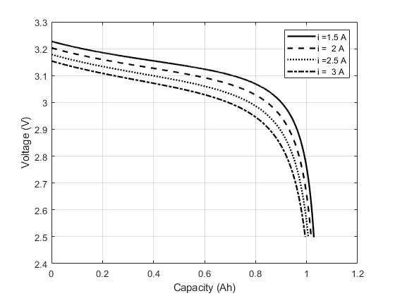
Figure 5. Zippy 1100mAh 2s (6.6V)- Simulation of voltage profile different discharge rates.
4.2 Test 2
Test 2 used a Turnigy Nano-Tech 1700mah 2s (6.6V), battery applying the same strategy as Test 1. The battery is discharged with a constant current of 1.1A, and Fig. 6 shows the parametric curve calculated using the algorithm.

Figure 6. Turnigy Nano-Tech 1700mah 2s (6.6V) - Comparison of experimental data with the optimised curve (i = 1.7A, T = 22ºC).
Table 3 shows the values calculated by the optimiser. The nominal capacity presented a difference of lower than 5%, and the estimated current difference was also lower than 2%. No parameter reached its bounds. Figure 7 shows the simulations discharging the battery with higher currents.
Table 3 Parameters obtained using the optimisation method and comparisons with nominal and measured data (Turnigy Nano-Tech 1700mah 2s (6.6V))

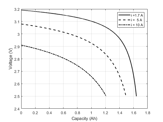
Figure 7. Turnigy Nano-Tech 1700mah 2s (6.6V) - Simulation of voltage profile for different discharge rates.
4.3 Test 3
Test 3 is important because it uses the current drawn from the motor in a real-life situation to find the discharge parameters for this configuration and calculate the real endurance of the aircraft. The Hacker TopFuel 4100mAh LiFePO4 4S battery was tested by controlling the current manually, moving the levers from the radio control, and visualising the current with a wattmeter, maintaining it as close as possible to 50A. Thus, using a different measurement set-up, shown in Fig. 8, Test 3 performs the battery discharge using a brushless motor from an aircraft. Figure 9 shows the parametric curve calculated using the algorithm.

Figure 8. Measurement set-up for Test 3.

Figure 9. Hacker TopFuel 4100mAh LiFePO44S - Comparison of experimental data with the optimised curve (i = 50A, T = 23ºC).
Table 4 shows the optimised parameters for Test 3. The nominal capacity presented a difference of 3% and the current difference of 5%. By analysing Fig. 10, up to a current of 50A, the capacity loss was lower than 8%.
Table 4 Parameters obtained using the optimisation method and comparisons with nominal and measured data (Hacker TopFuel 4100mAh LiFePO44S)


Figure 10. Hacker TopFuel 4100mAh LiFePO44S - Simulation of voltage profile for different discharge rates.
With the discharge profile already calculated, it is possible to make a more accurate estimate of flight time. To carry this out, the required power should be calculated using the aircraft parameters such as its drag and lift coefficients in each flight phase (i.e. takeoff, cruise, landing). With the required power is possible to estimate the current draw using the efficiency of the motor and propeller combined with battery voltage. A more direct route of obtaining this parameter is through direct measurement of the current in a flight test. Table 5 presents an estimation of the current in each flight phase. These values for current were inserted as inputs in the equation enabling the estimation of the flight time shown in Fig. 11.
Table 5 Current draw estimation for the aircraft in Fig. 8


Figure 11. Estimation of flight time for a UAV cargo used in SAE Brasil Aerodesign competition.
4.4 Validation and discussion
The optimisation code used only one discharge curve to parameterise the battery model. Though the parametric model appears to be very similar to the measured data, it is important to check if it can be applied with different discharge rates. Therefore, to validate the method, it was compared with the measured and simulated data for additional discharge rates for each test.
Figures 12-14 show the experimental and simulated curves for different discharge rates in the Zippy 1100mAh, Nano-Tech 1700mAh and Hacker TopFuel 4100m Ah respectively using a discharger with a controlled current.

Figure 12. Comparing simulation and experimental discharge for 0.6A, 2.4A, and 1.1A for the Zippy 1100mAh 2s (6.6V).

Figure 13. Comparing simulation and experimental discharge for 1A, 1.7A, 2.2A and 9A for the Zippy 1700mAh 2s (6.6V).

Figure 14. Comparing simulation and experimental discharge for 10A, 40A, 50A for the Hacker TopFuel 4100mAh LiFePO4 4S.
The gray area represents the precision error of the discharger used in the experiment. It can be seen that by the end of the experiment, the estimated endurance difference was 30s, 2.5min, and 2.1min, respectively, which means an error of 2.50%, 4.62%, and 1.96% for the Zippy 1100mAh. For the Nano-Tech 1700mAh battery, the difference was 30s, 2.5min, 30s, and 1.5min for 1.0A, 1.7A, 2.2A and 9A, respectively. This means an error of 0.50%, 6.09%, 0.97% and 1.63%, respectively. For the condition of 2.2A, the endurance error always remained lower than 1.0%. It is important to mention that the test with the 2.2A was performed on a different day to the other tests. A difference in environmental temperature could be a contributing factor. For the Hacker TopFuel 4100mAh, the difference was 12s, 23s, and 1min, respectively, which resulted in errors of 5.12%, 6.27%, and 4.65%.
Since this method uses a constrained multi-parameter optimisation, it also has advantages and limitations for this type of algorithm. In this model, the optimiser searches the best fit for the curve, which can lead to an unwanted trade-off between the optimisation parameters that generate a similar result (apparently), but are physically incorrect and will not work for different discharge rates. In this case, for example, the optimiser might find similar curves by increasing the internal resistance (R) and decreasing the polarisation constant (K) (or vice versa). To solve this issue, it is necessary to establish lower and upper limits for the optimisation variables in a way they do not converge on one of the bounds and stay constrained to a physically correct limit, which usually requires some trial-and-error set up for the limits.
The proposed model considers the discharge rate at a constant temperature. The aircraft in the present work flew around 10 minutes at a cruise height of 30m. The environmental temperature variation during the flights was no more than 10°C. Keil(Reference Keil14) performed experimental tests and showed that this variation (between 20°C and 30°C) could produce close to 4% of the capacity difference in a Li-ion battery. For the present experiment, this error can be accepted as a simplification, but for flight envelopes, with bigger differences, the model should be enhanced considering the temperature change(Reference Saw, Somasundaram, Ye and Tay9).
Also, the method uses only one discharge curve to fit the parameters of the model, so its precision will be limited by the quality of the experiment which must provide all parts of the curve (exponential, nominal, and terminal zone). The dynamic of discharge at higher rates can be rather different than at lower rates caused by effects not considered in the model such as the Peukert Effect. As can be seen in the 9A discharge (Fig. 13) and 10A (Fig. 14), the shape of the curve is slightly different from the experimental data. This is a consequence of the difference in rate compared when the parameters were extracted. The closer the simulation is to the fitted discharge curve, the more precise the results is. Therefore, the rate applied in the method should be as close as possible to the operational rate.
On the other hand, this algorithm is a powerful tool to provide both a fast and precise estimation of battery characteristics. Tremblay and Dessaint(Reference Tremblay and Dessaint10) proposed a method to estimate the parameters using datasheet values and three points from an experimental discharge curve, which lead to a 5.0% error between 100% and 20% of the state of charge (SOC) increasing the error to 10% for lower SOC values. Their validation only covered rates between 1C and 5C.
In the present results, Fig. 12 shows that the error of the simulated voltage was lower than 2.0% of the measured voltage during discharge with a slight increase in lower SOC values as it does not consider the Peukert Effect(Reference Tremblay and Dessaint10). In Fig. 13, the simulated voltage error remained lower than 2.0% for all SOCs. In Fig. 14, the voltage error remained lower than 2% increase to 3% for the lower 20% of the SOC for the 10A. These results provided a better endurance estimation and lower voltage error when compared with the manual method. It also expanded the analysis to higher rates (0.6C to 12.2C).
In short, this method brings precise results even with its simplifications and assumptions. Furthermore, datasheet parameters are not necessary to perform this estimation since the only input is the constant voltage (E0), which can be found by looking at the experimental discharge curve for a low discharge rate, which facilitates the identification of unknown batteries.
5.0 CONCLUSION
The estimation of the battery parameters using the setup described in this work proved to be an accurate tool to find the voltage drop curve and, consequently, the endurance of the aircraft. The same algorithm was tested using three different batteries, the capacity and current errors remained lower than 5.0%. The endurance estimation of the aircraft in Test 3 was carried out by estimating the current in each flight phase and summing their capacity, which generates a simplified voltage profile for a flight mission. The model was validated with different discharge rates in a controlled environment, which resulted in endurance errors lower than 6.0% for most of the conditions and a voltage estimation error lower than 2.0% for the operational voltage. These results proved the validity of the method which resulted in a better estimation when compared with a manual method.
An in-flight validation would be interesting as future work to understand the voltage dynamic of an uncontrolled environment. Another interesting analysis would be comparing a new battery with an old and swollen one to understand the effects of aging and bad usage. Lastly, an alternative method would be to use the optimiser not only with one discharge curve but instead three or more discharge curves to find the best-parametrised coefficients to fit all of them.


