


1 Introduction
The autoignition of turbulent fuel jets at elevated pressures and temperatures occurs in compression ignition engines such as diesel engines. Ignition is an important process in diesel combustion that influences flame stabilisation, which in turn affects pollutant formation and fuel conversion efficiency. For conventional diesel engine conditions, ignition occurs following the liquid injection of a high-velocity fuel jet into a high pressure and high-temperature environment. A two-staged autoignition then occurs, involving low-temperature chemistry (LTC) after the first-stage ignition delay time,
 $\unicode[STIX]{x1D70F}_{1}$
, and high-temperature chemistry (HTC) after the second-stage ignition delay time,
$\unicode[STIX]{x1D70F}_{1}$
, and high-temperature chemistry (HTC) after the second-stage ignition delay time,
 $\unicode[STIX]{x1D70F}$
(Pickett, Siebers & Idicheria Reference Pickett, Siebers and Idicheria2005; Idicheria & Pickett Reference Idicheria and Pickett2006; Pickett, Kook & Williams Reference Pickett, Kook and Williams2009). Following autoignition, a pseudo-stable, lifted flame is established (Dec Reference Dec1997). The distance between the injector and the flame base of the lifted flame is defined to be the lift off length (LOL). The location of autoignition and flame propagation in mixture-fraction (
$\unicode[STIX]{x1D70F}$
(Pickett, Siebers & Idicheria Reference Pickett, Siebers and Idicheria2005; Idicheria & Pickett Reference Idicheria and Pickett2006; Pickett, Kook & Williams Reference Pickett, Kook and Williams2009). Following autoignition, a pseudo-stable, lifted flame is established (Dec Reference Dec1997). The distance between the injector and the flame base of the lifted flame is defined to be the lift off length (LOL). The location of autoignition and flame propagation in mixture-fraction (
 $\unicode[STIX]{x1D709}$
) space is fuel and case dependent.
$\unicode[STIX]{x1D709}$
) space is fuel and case dependent.
Measurements of optically accessible diesel engines and chambers have been performed which have informed the development of conceptual models for diesel combustion (Dec Reference Dec1997; Idicheria & Pickett Reference Idicheria and Pickett2006; Musculus, Miles & Pickett Reference Musculus, Miles and Pickett2013; Maes et al. Reference Maes, Meijer, Dam, Somers, Toda, Bruneaux, Skeen, Pickett and Manin2016). At conventional diesel engine conditions, pre-ignition reactions due to LTC are observed, followed by the main ignition due to HTC. The HTC ignition appears to occur as a distributed event, originating from an ensemble of ignition locations (kernels) within the fuel rich and high velocity region of the jet (Dec Reference Dec1997). Ignition then proceeds towards leaner mixtures, and a non-premixed (diffusion) flame is established as the ignition front crosses the stoichiometric mixture fraction isosurface. The flame tends towards a pseudo-steady state such that the LOL is statistically steady. Recent large-eddy simulations (LES) of diesel spray combustion have reproduced these qualitative features and identified the effect of the LTC causing HTC ignition to occur in a rich mixture within the jet core (Gong, Jangi & Bai Reference Gong, Jangi and Bai2014). However, the stabilisation mechanism for diesel flames has not been conclusively demonstrated.
Siebers & Higgins (Reference Siebers and Higgins2001) and Siebers, Higgins & Pickett (Reference Siebers, Higgins and Pickett2002) observed that the variation in LOL could be explained by power laws derived from flame propagation scaling arguments for lifted flames at atmospheric conditions proposed by Peters (Reference Peters2001). This implied that the diesel flame was stabilised essentially by a propagation mechanism (either a premixed flame (Vanquickenborne & van Tiggelen Reference Vanquickenborne and van Tiggelen1966) or a partially premixed edge flame (Müller, Breitbach & Peters Reference Müller, Breitbach and Peters1994; Buckmaster Reference Buckmaster2002)). However, a subsequent study by Pickett et al. (Reference Pickett, Siebers and Idicheria2005) using Arrhenius law expressions for
 $\unicode[STIX]{x1D70F}$
, successfully explained the same trends as an autoignition controlled process. It is also possible that both stabilisation mechanisms contribute simultaneously, and/or the mechanism is dependent upon the operating conditions. The actual behaviour of the ignition and stabilisation processes is important to understand, as it would inform the appropriate selection of a suitable modelling framework when investigating diesel combustion.
$\unicode[STIX]{x1D70F}$
, successfully explained the same trends as an autoignition controlled process. It is also possible that both stabilisation mechanisms contribute simultaneously, and/or the mechanism is dependent upon the operating conditions. The actual behaviour of the ignition and stabilisation processes is important to understand, as it would inform the appropriate selection of a suitable modelling framework when investigating diesel combustion.
For atmospheric conditions, high-resolution experimental and numerical observations exist for non-premixed single-stage autoignition, e.g. see the review article by Mastorakos (Reference Mastorakos2009). Mastorakos, Baritaud & Poinsot (Reference Mastorakos, Baritaud and Poinsot1997) identified important properties of autoignition for laminar and turbulent non-premixed and partially premixed conditions. For laminar conditions, there exists a most reactive mixture-fraction value (
 $\unicode[STIX]{x1D709}_{MR}$
) (Mastorakos et al.
Reference Mastorakos, Baritaud and Poinsot1997) which has the shortest
$\unicode[STIX]{x1D709}_{MR}$
) (Mastorakos et al.
Reference Mastorakos, Baritaud and Poinsot1997) which has the shortest
 $\unicode[STIX]{x1D70F}$
and is therefore the preferred location of autoignition in composition space. The autoignition occurs first at
$\unicode[STIX]{x1D70F}$
and is therefore the preferred location of autoignition in composition space. The autoignition occurs first at
 $\unicode[STIX]{x1D709}_{MR}$
and then propagates into richer and leaner mixtures, including the
$\unicode[STIX]{x1D709}_{MR}$
and then propagates into richer and leaner mixtures, including the
 $\unicode[STIX]{x1D709}_{ST}$
value. At turbulent conditions, where fluctuations in the scalar dissipation rates (
$\unicode[STIX]{x1D709}_{ST}$
value. At turbulent conditions, where fluctuations in the scalar dissipation rates (
 $\unicode[STIX]{x1D712}$
) conditioned upon
$\unicode[STIX]{x1D712}$
) conditioned upon
 $\unicode[STIX]{x1D709}$
exist, ignition occurs first at locations near the
$\unicode[STIX]{x1D709}$
exist, ignition occurs first at locations near the
 $\unicode[STIX]{x1D709}_{MR}$
value where
$\unicode[STIX]{x1D709}_{MR}$
value where
 $\unicode[STIX]{x1D712}$
values are near the conditional minimum (Mastorakos et al.
Reference Mastorakos, Baritaud and Poinsot1997; Im, Chen & Law Reference Im, Chen and Law1998; Cao & Echekki Reference Cao and Echekki2007). Direct numerical simulation (DNS) studies have demonstrated that this phenomenon is related to the turbulent flow field such that ignition kernels tend to form in low dissipation regions such as the interior of vortices (Sreedhara & Lakshmisha Reference Sreedhara and Lakshmisha2000, Reference Sreedhara and Lakshmisha2002; Viggiano Reference Viggiano2004, Reference Viggiano2010). Echekki & Chen (Reference Echekki and Chen2002) also showed the establishment of lean and rich expanding premixed flames following autoignition which led to edge flames when the stoichiometric mixture fraction was crossed.
$\unicode[STIX]{x1D712}$
values are near the conditional minimum (Mastorakos et al.
Reference Mastorakos, Baritaud and Poinsot1997; Im, Chen & Law Reference Im, Chen and Law1998; Cao & Echekki Reference Cao and Echekki2007). Direct numerical simulation (DNS) studies have demonstrated that this phenomenon is related to the turbulent flow field such that ignition kernels tend to form in low dissipation regions such as the interior of vortices (Sreedhara & Lakshmisha Reference Sreedhara and Lakshmisha2000, Reference Sreedhara and Lakshmisha2002; Viggiano Reference Viggiano2004, Reference Viggiano2010). Echekki & Chen (Reference Echekki and Chen2002) also showed the establishment of lean and rich expanding premixed flames following autoignition which led to edge flames when the stoichiometric mixture fraction was crossed.
A series of experiments at atmospheric conditions were conducted by Markides & Mastorakos (Reference Markides and Mastorakos2005), Markides, De Paola & Mastorakos (Reference Markides, De Paola and Mastorakos2007), Markides & Mastorakos (Reference Markides and Mastorakos2011) for turbulent non-premixed jets featuring autoignition using hydrogen, n-heptane and acetylene, respectively. A statistically stationary state was achieved in each study, such that a rapid succession of autoignition kernels was observed that did not lead to a continuously burning flame. This was termed the ‘random spots’ regime (Markides & Mastorakos Reference Markides and Mastorakos2005). Tracking of individual kernels was conducted. Rapid kernel growth was observed leading to individual flamelets that later merged or were extinguished. The flamelets resembled tribrachial (triple) flames, which have a main crescent-shaped front composed of premixed lean and rich branches and a trailing non-premixed (diffusion) flame branch. The results for the hydrogen case were later reproduced in a DNS study by Kerkemeier et al. (Reference Kerkemeier, Markides, Frouzakis and Boulouchos2013). The DNS results showed the following: that the ignition kernels formed near the
 $\unicode[STIX]{x1D709}_{MR}$
value, with low
$\unicode[STIX]{x1D709}_{MR}$
value, with low
 $\unicode[STIX]{x1D712}$
; that increasing levels of turbulence suppressed the formation of the ignition kernels; and that autoignition and flame propagation modes could coexist in a statistically stationary ignition case.
$\unicode[STIX]{x1D712}$
; that increasing levels of turbulence suppressed the formation of the ignition kernels; and that autoignition and flame propagation modes could coexist in a statistically stationary ignition case.
Numerical (Lyra et al.
Reference Lyra, Wilde, Kolla, Seitzman, Lieuwen and Chen2015) and experimental (Micka & Driscoll Reference Micka and Driscoll2012; Fleck et al.
Reference Fleck, Griebel, Steinberg, Arndt and Aigner2013a
,Reference Fleck, Griebel, Steinberg, Arndt, Naumann and Aigner
b
; Sullivan et al.
Reference Sullivan, Wilde, Noble, Seitzman and Lieuwen2014) investigations have been performed for autoignition in shear flows for the jet in cross-flow (JICF) configuration. Several of these studies (Micka & Driscoll Reference Micka and Driscoll2012; Sullivan et al.
Reference Sullivan, Wilde, Noble, Seitzman and Lieuwen2014; Lyra et al.
Reference Lyra, Wilde, Kolla, Seitzman, Lieuwen and Chen2015) considered the stabilisation mechanism and time-averaged structure of autoignitive JICF flames, which is not the focus of the present temporally evolving study. High-speed imaging performed by Fleck et al. (Reference Fleck, Griebel, Steinberg, Arndt and Aigner2013a
,Reference Fleck, Griebel, Steinberg, Arndt, Naumann and Aigner
b
) at elevated pressure with hydrogen/nitrogen jets observed a transient ignition processes with many independent ignition kernels. Some kernels were advected out of the combustor (blow off), while others successfully produced a stabilised flame. An overlap in the spatial distribution of successful and unsuccessful ignition kernels was observed. This was attributed to fluctuations in: mean turbulent structure, local mixing rates and local thermochemical fluctuations, however it was not possible to directly measure these effects with respect to each ignition kernel as resolved measurements of the
 $\unicode[STIX]{x1D709}$
and
$\unicode[STIX]{x1D709}$
and
 $\unicode[STIX]{x1D712}$
were not available. Fleck et al. (Reference Fleck, Griebel, Steinberg, Arndt and Aigner2013a
) further distinguished between primary and secondary ignition kernels. Primary ignition kernels were those that formed in the absence of other ignition sources in the domain while secondary kernels occurred in the presence of combustion elsewhere in the domain. For most cases it was observed that primary kernels did not in themselves establish a stabilised flame but that they influenced the fluid mechanical and mixing fields in a manner that promoted the formation and success of secondary ignition kernels.
$\unicode[STIX]{x1D712}$
were not available. Fleck et al. (Reference Fleck, Griebel, Steinberg, Arndt and Aigner2013a
) further distinguished between primary and secondary ignition kernels. Primary ignition kernels were those that formed in the absence of other ignition sources in the domain while secondary kernels occurred in the presence of combustion elsewhere in the domain. For most cases it was observed that primary kernels did not in themselves establish a stabilised flame but that they influenced the fluid mechanical and mixing fields in a manner that promoted the formation and success of secondary ignition kernels.
Resolved measurements of temperature and mixture fraction for impulsively forced methane jets in a hot coflow burner have been performed by Papageorge et al. (Reference Papageorge, Arndt, Fuest, Meier and Sutton2014) and Arndt et al. (Reference Arndt, Papageorge, Fuest, Sutton, Meier and Aigner2016). The location of the formation of ignition kernels in
 $\unicode[STIX]{x1D709}$
and
$\unicode[STIX]{x1D709}$
and
 $\unicode[STIX]{x1D712}$
space was measured for an ensemble of injection events. It was observed that most of the ignition kernels formed in the periphery of the jet, in mixtures with
$\unicode[STIX]{x1D712}$
space was measured for an ensemble of injection events. It was observed that most of the ignition kernels formed in the periphery of the jet, in mixtures with
 $\unicode[STIX]{x1D709}<\unicode[STIX]{x1D709}_{ST}$
and experiencing low
$\unicode[STIX]{x1D709}<\unicode[STIX]{x1D709}_{ST}$
and experiencing low
 $\unicode[STIX]{x1D712}$
, which was in good agreement with prior DNS of autoignition with single-stage ignition chemistry (Mastorakos Reference Mastorakos2009).
$\unicode[STIX]{x1D712}$
, which was in good agreement with prior DNS of autoignition with single-stage ignition chemistry (Mastorakos Reference Mastorakos2009).
It is difficult to directly compare ignition studies conducted at low to moderate pressures and with single-stage ignition chemistry to diesel-engine-relevant conditions due to the weakness of two-stage ignition and negative temperature coefficient (NTC). (Two-stage ignition can be observed at atmospheric and moderately elevated pressures, however, over the temperature range it occurs the corresponding ignition delays are very long, more than 10 ms for large n-alkanes.) Recently, several two-dimensional (2-D) DNS studies were conducted at diesel-relevant thermochemical conditions using the oxygenated fuel dimethyl ether (Deng et al.
Reference Deng, Zhao, Mueller and Law2015a
,Reference Deng, Zhao, Mueller and Law
b
; Krisman et al.
Reference Krisman, Hawkes, Talei, Bhagatwala and Chen2015, Reference Krisman, Hawkes, Talei, Bhagatwala and Chen2016, Reference Krisman, Hawkes, Talei, Bhagatwala and Chen2017), for a lifted laminar flame (Deng et al.
Reference Deng, Zhao, Mueller and Law2015a
,Reference Deng, Zhao, Mueller and Law
b
; Krisman et al.
Reference Krisman, Hawkes, Talei, Bhagatwala and Chen2015) and pseudo-turbulent mixing layer (Krisman et al.
Reference Krisman, Hawkes, Talei, Bhagatwala and Chen2016, Reference Krisman, Hawkes, Talei, Bhagatwala and Chen2017) configuration. Krisman et al. (Reference Krisman, Hawkes, Talei, Bhagatwala and Chen2015) identified polybrachial edge flames that exhibit characteristics of both edge-flame propagation (a main tribrachial flame) and autoignition (observed in additional upstream branches due to LTC and/or HTC autoignition). The branch structure of the polybrachial flames is related to the homogeneous ignition delay times of both the first stage (
 $\unicode[STIX]{x1D70F}_{1}$
) and the second stage (
$\unicode[STIX]{x1D70F}_{1}$
) and the second stage (
 $\unicode[STIX]{x1D70F}$
) of autoignition, and their respective most reactive mixture-fraction values (
$\unicode[STIX]{x1D70F}$
) of autoignition, and their respective most reactive mixture-fraction values (
 $\unicode[STIX]{x1D709}_{MR,1}$
and
$\unicode[STIX]{x1D709}_{MR,1}$
and
 $\unicode[STIX]{x1D709}_{MR}$
). A subsequent study by Deng et al. (Reference Deng, Zhao, Mueller and Law2015a
) used a chemical explosive mode analysis (CEMA) (Lu et al.
Reference Lu, Yoo, Chen and Law2010) to provide additional support for the hybrid premixed/autoignitive character of the polybrachial flames.
$\unicode[STIX]{x1D709}_{MR}$
). A subsequent study by Deng et al. (Reference Deng, Zhao, Mueller and Law2015a
) used a chemical explosive mode analysis (CEMA) (Lu et al.
Reference Lu, Yoo, Chen and Law2010) to provide additional support for the hybrid premixed/autoignitive character of the polybrachial flames.
The lifted laminar 2-D DNS studies did not consider turbulence effects, which may influence the ignition and stabilisation process. An important effect of turbulence for non-premixed conditions is that it produces conditional fluctuations of
 $\unicode[STIX]{x1D712}$
in
$\unicode[STIX]{x1D712}$
in
 $\unicode[STIX]{x1D709}$
-space. In order to study this effect, a simulation was performed for a 2-D dimethyl ether-air mixing layer in isotropic pseudo-turbulence (Krisman et al.
Reference Krisman, Hawkes, Talei, Bhagatwala and Chen2017) for thermochemical conditions identical to the
$\unicode[STIX]{x1D709}$
-space. In order to study this effect, a simulation was performed for a 2-D dimethyl ether-air mixing layer in isotropic pseudo-turbulence (Krisman et al.
Reference Krisman, Hawkes, Talei, Bhagatwala and Chen2017) for thermochemical conditions identical to the
 $T_{OX}=900$
K case from Krisman et al. (Reference Krisman, Hawkes, Talei, Bhagatwala and Chen2015). In that study, a mixing field with a Damköhler number (Da) of 0.4 was imposed over an initially laminar mixing layer profile. The
$T_{OX}=900$
K case from Krisman et al. (Reference Krisman, Hawkes, Talei, Bhagatwala and Chen2015). In that study, a mixing field with a Damköhler number (Da) of 0.4 was imposed over an initially laminar mixing layer profile. The
 $Da$
value was selected in order to approximate the value calculated from simulations of igniting n-dodecane sprays near the flame stabilisation location (Pei et al.
Reference Pei, Hawkes, Bolla, Kook, Goldin, Yang, Pope and Som2016). An investigation of the LTC behaviour identified that the first stage of autoignition transitions to a diffusively supported cool flame that moves up the local mixture-fraction gradient towards richer mixtures much faster than expected from spatial gradients in the first-stage ignition delay time. The cool flame advances the timing of the LTC heat release, shortening the main ignition delay time,
$Da$
value was selected in order to approximate the value calculated from simulations of igniting n-dodecane sprays near the flame stabilisation location (Pei et al.
Reference Pei, Hawkes, Bolla, Kook, Goldin, Yang, Pope and Som2016). An investigation of the LTC behaviour identified that the first stage of autoignition transitions to a diffusively supported cool flame that moves up the local mixture-fraction gradient towards richer mixtures much faster than expected from spatial gradients in the first-stage ignition delay time. The cool flame advances the timing of the LTC heat release, shortening the main ignition delay time,
 $\unicode[STIX]{x1D70F}$
, which is in good agreement with prior LES observations (Gong et al.
Reference Gong, Jangi and Bai2014), inferences from transported probability density function models (Pei et al.
Reference Pei, Hawkes, Bolla, Kook, Goldin, Yang, Pope and Som2016) and an independent study by Dahms et al. (Reference Dahms, Paczko, Skeen and Pickett2017) in the context of turbulent n-dodecane ignition modelled with a Lagrangian flamelet method. A detailed study of the overall ignition dynamics for the same dataset in Krisman et al. (Reference Krisman, Hawkes, Talei, Bhagatwala and Chen2017) was also performed (Krisman et al.
Reference Krisman, Hawkes, Talei, Bhagatwala and Chen2016). A very complex ignition was observed such that multiple stages of autoignition and multiple modes of combustion were identified. The results suggested that both autoignition and edge-flame propagation can both be prominent at diesel-relevant conditions, which has implications for practical modelling of diesel engines.
$\unicode[STIX]{x1D70F}$
, which is in good agreement with prior LES observations (Gong et al.
Reference Gong, Jangi and Bai2014), inferences from transported probability density function models (Pei et al.
Reference Pei, Hawkes, Bolla, Kook, Goldin, Yang, Pope and Som2016) and an independent study by Dahms et al. (Reference Dahms, Paczko, Skeen and Pickett2017) in the context of turbulent n-dodecane ignition modelled with a Lagrangian flamelet method. A detailed study of the overall ignition dynamics for the same dataset in Krisman et al. (Reference Krisman, Hawkes, Talei, Bhagatwala and Chen2017) was also performed (Krisman et al.
Reference Krisman, Hawkes, Talei, Bhagatwala and Chen2016). A very complex ignition was observed such that multiple stages of autoignition and multiple modes of combustion were identified. The results suggested that both autoignition and edge-flame propagation can both be prominent at diesel-relevant conditions, which has implications for practical modelling of diesel engines.
Several other high-resolution studies have been performed for diesel-relevant ignition (Sreedhara & Lakshmisha Reference Sreedhara and Lakshmisha2002; Viggiano Reference Viggiano2004, Reference Viggiano2010; Mukhopadhyay & Abraham Reference Mukhopadhyay and Abraham2012b
; Borghesi, Mastorakos & Cant Reference Borghesi, Mastorakos and Cant2013; Minamoto & Chen Reference Minamoto and Chen2016). Sreedhara & Lakshmisha (Reference Sreedhara and Lakshmisha2002) conducted a 3-D DNS of autoignition at engine-relevant thermochemical conditions for a domain of decaying isotropic turbulence. The simulations used a global chemical mechanism for n-heptane that models both the LTC and HTC reactions (Müller & Peters Reference Müller and Peters1992). The results identified that ignition occurred in regions near
 $\unicode[STIX]{x1D709}_{MR}$
where
$\unicode[STIX]{x1D709}_{MR}$
where
 $\unicode[STIX]{x1D712}$
is low, which corresponded to flow topologies that were judged to be vortically dominated, similar to previous observations for the autoignition of non-premixed vortex-mixing layer interactions at atmospheric pressure by Thévenin & Candel (Reference Thévenin and Candel1995). However, in the study by Sreedhara & Lakshmisha (Reference Sreedhara and Lakshmisha2002), individual ignition kernels were not identified; rather, ignition was identified by ensemble-averaged statistics, which showed a broad region of ignition in
$\unicode[STIX]{x1D712}$
is low, which corresponded to flow topologies that were judged to be vortically dominated, similar to previous observations for the autoignition of non-premixed vortex-mixing layer interactions at atmospheric pressure by Thévenin & Candel (Reference Thévenin and Candel1995). However, in the study by Sreedhara & Lakshmisha (Reference Sreedhara and Lakshmisha2002), individual ignition kernels were not identified; rather, ignition was identified by ensemble-averaged statistics, which showed a broad region of ignition in
 $\unicode[STIX]{x1D709}$
space. Furthermore, the measurement of ignition with respect to flow topology was conducted for stoichiometric mixtures, not for the most reactive mixtures where autoignition was known to occur. Borghesi et al. (Reference Borghesi, Mastorakos and Cant2013) performed a DNS of n-heptane droplet autoignition at a pressure of 24 atmospheres using a chemical mechanism with 18 global steps. A spotty ignition pattern was observed and doubly conditioned statistics demonstrated that kernel formation favoured
$\unicode[STIX]{x1D709}$
space. Furthermore, the measurement of ignition with respect to flow topology was conducted for stoichiometric mixtures, not for the most reactive mixtures where autoignition was known to occur. Borghesi et al. (Reference Borghesi, Mastorakos and Cant2013) performed a DNS of n-heptane droplet autoignition at a pressure of 24 atmospheres using a chemical mechanism with 18 global steps. A spotty ignition pattern was observed and doubly conditioned statistics demonstrated that kernel formation favoured
 $\unicode[STIX]{x1D709}_{MR}$
locations where
$\unicode[STIX]{x1D709}_{MR}$
locations where
 $\unicode[STIX]{x1D712}$
values are low. The importance of macro-mixing was also emphasised, since the formation of regions with
$\unicode[STIX]{x1D712}$
values are low. The importance of macro-mixing was also emphasised, since the formation of regions with
 $\unicode[STIX]{x1D709}\approx \unicode[STIX]{x1D709}_{MR}$
assist early ignition, which may be affected by many factors including mixing time, evaporation rates and turbulence intensity. Recently Minamoto & Chen (Reference Minamoto and Chen2016) conducted a 3-D DNS study of a turbulent lifted flame at NTC conditions. In order to reduce the computational expense of the simulation, a partially reacted mixture was imposed at the inlet in order to represent the products of the LTC reactions. This approach reduced the residence time (and hence domain size) requirements, which made the use of DNS tractable. The turbulent flow disrupted the laminar flame structures observed by Krisman et al. (Reference Krisman, Hawkes, Talei, Bhagatwala and Chen2015). However, appropriate conditioning of the results revealed the same polybrachial flame structure observed in the laminar case. Measurements of displacement speeds were also performed that indicated that the presence of LTC reactions substantially enhances the displacement speeds. The main limitation of this study was the use of the partially reacted inflow which precluded the study of the two-stage ignition process.
$\unicode[STIX]{x1D709}\approx \unicode[STIX]{x1D709}_{MR}$
assist early ignition, which may be affected by many factors including mixing time, evaporation rates and turbulence intensity. Recently Minamoto & Chen (Reference Minamoto and Chen2016) conducted a 3-D DNS study of a turbulent lifted flame at NTC conditions. In order to reduce the computational expense of the simulation, a partially reacted mixture was imposed at the inlet in order to represent the products of the LTC reactions. This approach reduced the residence time (and hence domain size) requirements, which made the use of DNS tractable. The turbulent flow disrupted the laminar flame structures observed by Krisman et al. (Reference Krisman, Hawkes, Talei, Bhagatwala and Chen2015). However, appropriate conditioning of the results revealed the same polybrachial flame structure observed in the laminar case. Measurements of displacement speeds were also performed that indicated that the presence of LTC reactions substantially enhances the displacement speeds. The main limitation of this study was the use of the partially reacted inflow which precluded the study of the two-stage ignition process.
To the best of the authors’ knowledge, no fully resolved studies exist that included both diesel-engine-relevant thermochemical conditions (leading to two-stage ignition) and realistic, 3-D turbulence. On the experimental side, this is due to the extreme challenge of obtaining well resolved measurements at diesel engine conditions. For experimental studies, the high pressure and temperature environment combined with the extremely small spatial scales and fast time scales (in addition to other challenges such as multiphase flow effects), inhibit the collection of fully resolved measurements. For numerical studies, DNS studies are limited by computational cost, which scales with the third power of the range of simulated scales and linearly with the range of temporal scales. Consequently, any 3-D DNS study is computationally expensive and existing databases are limited to statistically small computational domains with physically unrepresentative isotropic, decaying turbulence (Sreedhara & Lakshmisha Reference Sreedhara and Lakshmisha2002; Borghesi et al. Reference Borghesi, Mastorakos and Cant2013) or do not include the LTC dynamics (Minamoto & Chen Reference Minamoto and Chen2016).
The approach in the present study is to make appropriate simplifying assumptions while focusing on interactions between the two-stage ignition, edge-flame propagation and the flow topology. The major simplifying assumption is the use of a global n-heptane chemical mechanism in place of a detailed mechanism with elementary reactions, while three-dimensionality and realistic turbulence are retained. The mechanism used here, by Müller & Peters (Reference Müller and Peters1992), has been previously used in DNS of diesel-engine-relevant conditions in order to reduce the computational cost (Sreedhara & Lakshmisha Reference Sreedhara and Lakshmisha2002; Viggiano Reference Viggiano2004). Without this simplifying assumption the simulation would not have been feasible, even on leading high performance computing facilities.
In this study, a temporally evolving turbulent slot jet of n-heptane fuel is surrounded by initially stagnant oxidiser. The initial conditions produce a two-stage autoignition in the presence of shear-driven turbulence. The turbulence produces intense mixing between the fuel and oxidiser which leads to large conditional fluctuations of
 $\unicode[STIX]{x1D712}$
in
$\unicode[STIX]{x1D712}$
in
 $\unicode[STIX]{x1D709}$
-space. The main aim of the simulation is to study the ignition dynamics in the presence of both LTC and HTC, subject to realistic, shear-driven turbulence. In particular, the connections between combustion modes, mixing and the flow topology are explored. The use of Lagrangian tracer particles allows for an examination of the ignition kernels time histories prior to autoignition. This is used here to investigate the effects of mixing and flow topology on the autoignition event. The present study details both the development of individual combustion features and the evolution of the statistically 1-D flame.
$\unicode[STIX]{x1D709}$
-space. The main aim of the simulation is to study the ignition dynamics in the presence of both LTC and HTC, subject to realistic, shear-driven turbulence. In particular, the connections between combustion modes, mixing and the flow topology are explored. The use of Lagrangian tracer particles allows for an examination of the ignition kernels time histories prior to autoignition. This is used here to investigate the effects of mixing and flow topology on the autoignition event. The present study details both the development of individual combustion features and the evolution of the statistically 1-D flame.
2 Methodology
2.1 Numerical method
The DNS was conducted with the code S3D (Chen et al. Reference Chen, Choudhary, de Supinski, DeVries, Hawkes, Klasky, Liao, Ma, Mellor-Crummey and Podhorszki2009). S3D solves the conservation equations for the compressible Navier–Stokes, continuity, total energy and species mass fraction equations with a high-order accurate, non-dissipative finite difference scheme. Spatial derivatives are approximated with an eighth-order central finite difference scheme and temporal integration is performed with a fourth-order, six-stage explicit Runge–Kutta method. Spurious high-wavenumber oscillations were removed with a tenth-order explicit filter (Kennedy & Carpenter Reference Kennedy and Carpenter1994) that is applied once every 10 time steps. S3D has been used in many DNS studies of turbulent combustion (Im et al. Reference Im, Chen and Law1998; Echekki & Chen Reference Echekki and Chen2002; Sankaran et al. Reference Sankaran, Hawkes, Chen, Lu and Law2007, Reference Sankaran, Hawkes, Yoo and Chen2015; Wang & Rutland Reference Wang and Rutland2007; Chen et al. Reference Chen, Choudhary, de Supinski, DeVries, Hawkes, Klasky, Liao, Ma, Mellor-Crummey and Podhorszki2009; Yoo et al. Reference Yoo, Richardson, Sankaran and Chen2011; Chatakonda et al. Reference Chatakonda, Hawkes, Aspden, Kerstein, Kolla and Chen2013; Karami et al. Reference Karami, Hawkes, Talei and Chen2015, Reference Karami, Hawkes, Talei and Chen2016), including studies of temporally evolving non-premixed slot-jet flames (Hawkes et al. Reference Hawkes, Sankaran, Sutherland and Chen2007; Lignell, Chen & Smith Reference Lignell, Chen and Smith2008), which is the configuration used in the present simulation. The mixture specific heat and viscosity transport properties were calculated based on the local temperature and composition, assuming unity Lewis numbers for all species.
2.2 Configuration
A diagram of the domain is presented in figure 1. The domain consists of a slot jet of fuel between stationary layers of oxidiser at a pressure of 40 atmospheres. The fuel is pure n-heptane at 400 K and the oxidiser composition is 79 %
 $\text{N}_{2}$
and 21 %
$\text{N}_{2}$
and 21 %
 $\text{O}_{2}$
by volume at 1100 K. The profile of the jet is defined in terms of the mixture fraction,
$\text{O}_{2}$
by volume at 1100 K. The profile of the jet is defined in terms of the mixture fraction,
 $\unicode[STIX]{x1D709}$
:
$\unicode[STIX]{x1D709}$
:
 $\unicode[STIX]{x1D709}(y)=0.5(\tanh ((y+H_{JET}/2)/\unicode[STIX]{x1D70E})-\tanh ((y-H_{JET}/2)/\unicode[STIX]{x1D70E}))$
, where the profile thickness is
$\unicode[STIX]{x1D709}(y)=0.5(\tanh ((y+H_{JET}/2)/\unicode[STIX]{x1D70E})-\tanh ((y-H_{JET}/2)/\unicode[STIX]{x1D70E}))$
, where the profile thickness is
 $\unicode[STIX]{x1D70E}=H_{JET}/8$
, and where
$\unicode[STIX]{x1D70E}=H_{JET}/8$
, and where
 $H_{JET}$
is the jet width.
$H_{JET}$
is the jet width.
 $H_{JET}$
and the jet velocity,
$H_{JET}$
and the jet velocity,
 $U_{JET}$
, are constrained by the target jet Reynolds number,
$U_{JET}$
, are constrained by the target jet Reynolds number,
 $Re_{JET}=(H_{JET}U_{JET})/\unicode[STIX]{x1D708}_{JET}$
, and jet Damköhler number,
$Re_{JET}=(H_{JET}U_{JET})/\unicode[STIX]{x1D708}_{JET}$
, and jet Damköhler number,
 $Da_{JET}=(H_{JET}/U_{JET})/\unicode[STIX]{x1D70F}_{MR}$
, where
$Da_{JET}=(H_{JET}/U_{JET})/\unicode[STIX]{x1D70F}_{MR}$
, where
 $\unicode[STIX]{x1D708}_{JET}$
is the kinematic viscosity of pure fuel, equal to
$\unicode[STIX]{x1D708}_{JET}$
is the kinematic viscosity of pure fuel, equal to
 $1.94\times 10^{-7}~\text{m}^{2}~\text{s}^{-1}$
, and
$1.94\times 10^{-7}~\text{m}^{2}~\text{s}^{-1}$
, and
 $\unicode[STIX]{x1D70F}_{MR}$
is the homogeneous ignition delay time of the most reactive mixture fraction, equal to 0.28 ms.
$\unicode[STIX]{x1D70F}_{MR}$
is the homogeneous ignition delay time of the most reactive mixture fraction, equal to 0.28 ms.
 $Re_{JET}$
is constrained by computational cost and is set to 9000, which approaches the
$Re_{JET}$
is constrained by computational cost and is set to 9000, which approaches the
 $Re_{JET}$
of previous, moderately turbulent combustion DNS cases (Hawkes et al.
Reference Hawkes, Sankaran, Sutherland and Chen2007; Yoo, Sankaran & Chen Reference Yoo, Sankaran and Chen2009; Yoo et al.
Reference Yoo, Richardson, Sankaran and Chen2011).
$Re_{JET}$
of previous, moderately turbulent combustion DNS cases (Hawkes et al.
Reference Hawkes, Sankaran, Sutherland and Chen2007; Yoo, Sankaran & Chen Reference Yoo, Sankaran and Chen2009; Yoo et al.
Reference Yoo, Richardson, Sankaran and Chen2011).
 $Da_{JET}$
is set to 0.11, which was selected to approximately match the Da in the vicinity of autoignition in diesel conditions as calculated from Reynolds-averaged Navier–Stokes (RANS) simulations of n-dodecane flames (Pei et al.
Reference Pei, Hawkes, Bolla, Kook, Goldin, Yang, Pope and Som2016), and to appropriately time the autoignition with respect to the turbulent jet development in the present simulation. The timing of autoignition was very sensitive to
$Da_{JET}$
is set to 0.11, which was selected to approximately match the Da in the vicinity of autoignition in diesel conditions as calculated from Reynolds-averaged Navier–Stokes (RANS) simulations of n-dodecane flames (Pei et al.
Reference Pei, Hawkes, Bolla, Kook, Goldin, Yang, Pope and Som2016), and to appropriately time the autoignition with respect to the turbulent jet development in the present simulation. The timing of autoignition was very sensitive to
 $Da_{JET}$
in preliminary, under-resolved simulations of the present configuration.
$Da_{JET}$
in preliminary, under-resolved simulations of the present configuration.
 $Da_{JET}$
was selected to time the ignition after the development of turbulence due to shear, but well before the spreading of the jet reached the outflow boundaries. This allowed the jet to reach a burning state prior to the statistical saturation of the domain. These constraints result in an initial jet width of
$Da_{JET}$
was selected to time the ignition after the development of turbulence due to shear, but well before the spreading of the jet reached the outflow boundaries. This allowed the jet to reach a burning state prior to the statistical saturation of the domain. These constraints result in an initial jet width of
 $H_{JET}=0.233$
mm and an initial centreline velocity of
$H_{JET}=0.233$
mm and an initial centreline velocity of
 $U_{JET}=7.49~\text{m}~\text{s}^{-1}$
, which define the jet time of
$U_{JET}=7.49~\text{m}~\text{s}^{-1}$
, which define the jet time of
 $t_{JET}=31.1~\unicode[STIX]{x03BC}\text{s}$
. Non-dimensional parameters are defined for time,
$t_{JET}=31.1~\unicode[STIX]{x03BC}\text{s}$
. Non-dimensional parameters are defined for time,
 $t^{\ast }=t/t_{JET}$
, and spatial directions,
$t^{\ast }=t/t_{JET}$
, and spatial directions,
 $x^{\ast }=x/H_{JET}$
,
$x^{\ast }=x/H_{JET}$
,
 $y^{\ast }=y/H_{JET}$
, and
$y^{\ast }=y/H_{JET}$
, and
 $z^{\ast }=z/H_{JET}$
.
$z^{\ast }=z/H_{JET}$
.

Figure 1. Diagram of the domain configuration, including specification of the boundary and initial conditions. Blue circles represent the region initially seeded with passive fluid tracer particles.
The extent of the domain in the
 $x$
,
$x$
,
 $y$
and
$y$
and
 $z$
directions is chosen to be
$z$
directions is chosen to be
 $L_{x}=12H_{JET}$
,
$L_{x}=12H_{JET}$
,
 $L_{y}=18H_{JET},L_{z}=8H_{JET}$
, respectively. The domain size is adequate for the jet to develop and to obtain a sufficient statistical sample in the periodic directions, while minimising the computational expense. Superimposed on the initial condition is a spectrum of low-amplitude isotropic turbulence in order to excite the unstable jet. The isotropic turbulence has a velocity fluctuation scale of
$L_{y}=18H_{JET},L_{z}=8H_{JET}$
, respectively. The domain size is adequate for the jet to develop and to obtain a sufficient statistical sample in the periodic directions, while minimising the computational expense. Superimposed on the initial condition is a spectrum of low-amplitude isotropic turbulence in order to excite the unstable jet. The isotropic turbulence has a velocity fluctuation scale of
 $u^{\prime }/U_{JET}=0.05$
and an integral length scale of
$u^{\prime }/U_{JET}=0.05$
and an integral length scale of
 $L_{t}/H_{JET}=0.33$
. The fluctuations satisfied a Passot–Pouquet energy spectrum (Hinze Reference Hinze1975).
$L_{t}/H_{JET}=0.33$
. The fluctuations satisfied a Passot–Pouquet energy spectrum (Hinze Reference Hinze1975).
The boundary conditions are periodic in the streamwise (
 $x$
) and spanwise (
$x$
) and spanwise (
 $z$
) directions and non-reflecting outflows in the cross-stream (
$z$
) directions and non-reflecting outflows in the cross-stream (
 $y$
) direction, evaluated using the Navier–Stokes characteristic boundary condition method (NSCBC) (Poinsot Reference Poinsot1992). The grid count in each direction is
$y$
) direction, evaluated using the Navier–Stokes characteristic boundary condition method (NSCBC) (Poinsot Reference Poinsot1992). The grid count in each direction is
 $n_{x}=1440$
,
$n_{x}=1440$
,
 $n_{y}=1472$
and
$n_{y}=1472$
and
 $n_{z}=960$
, which is selected to properly resolve the smallest chemical and turbulent length scales. There are 81 points across the
$n_{z}=960$
, which is selected to properly resolve the smallest chemical and turbulent length scales. There are 81 points across the
 $H_{JET}$
, which is consistent with values selected in previous DNS of slot jets at similar
$H_{JET}$
, which is consistent with values selected in previous DNS of slot jets at similar
 $Re_{JET}$
values (Hawkes et al.
Reference Hawkes, Sankaran, Sutherland and Chen2007; Yoo et al.
Reference Yoo, Richardson, Sankaran and Chen2011). There are 0.72 grid points across the smallest Kolmogorov length scale,
$Re_{JET}$
values (Hawkes et al.
Reference Hawkes, Sankaran, Sutherland and Chen2007; Yoo et al.
Reference Yoo, Richardson, Sankaran and Chen2011). There are 0.72 grid points across the smallest Kolmogorov length scale,
 $\unicode[STIX]{x1D702}_{k}$
. This is sufficient as it exceeds suggested guidelines for DNS of turbulent flows (Pope Reference Pope2000), and the value reported from a previous, well-resolved slot-jet DNS case (Hawkes et al.
Reference Hawkes, Sankaran, Sutherland and Chen2007). In order to ensure that the chemical structure of the flame was resolved, a grid convergence test was conducted for a one-dimensional premixed flame, see figure 2. The results showed that the selected grid was sufficient to correctly resolve the premixed flame; in three dimensions, depending on the flame orientation, the best and worst case spacing is between 2 and 4 microns, respectively.
$\unicode[STIX]{x1D702}_{k}$
. This is sufficient as it exceeds suggested guidelines for DNS of turbulent flows (Pope Reference Pope2000), and the value reported from a previous, well-resolved slot-jet DNS case (Hawkes et al.
Reference Hawkes, Sankaran, Sutherland and Chen2007). In order to ensure that the chemical structure of the flame was resolved, a grid convergence test was conducted for a one-dimensional premixed flame, see figure 2. The results showed that the selected grid was sufficient to correctly resolve the premixed flame; in three dimensions, depending on the flame orientation, the best and worst case spacing is between 2 and 4 microns, respectively.

Figure 2. Grid convergence test result for lifted 1-D premixed flame at the most reactive mixture fraction for the conditions in this study. The lower left peak corresponds to the LTC ignition and the higher right peak corresponds to the high-temperature reaction zone. The inset shows the high-temperature reaction zone in detail. The grid resolutions noted in the legend have units of
 $\unicode[STIX]{x03BC}\text{m}$
.
$\unicode[STIX]{x03BC}\text{m}$
.
Fluid tracer particles were also embedded in the flow at the start of the simulation to aggregate Lagrangian statistics. Approximately 53.3 million particles were randomly placed at a uniform density within the central half of the cross-stream direction.
2.3 Chemistry model
A four-step, six-species global chemical mechanism for n-heptane was used, based on that first proposed by Müller & Peters (Reference Müller and Peters1992). The choice of global chemical reaction scheme was motivated by the need for a computationally inexpensive chemical mechanism. Since diesel engine conditions involve very high pressures, the reaction zone thicknesses and hence resolution requirements are onerous (e.g. requiring approximately 1 micron resolution or less for chemical mechanisms that include radical species and short lived intermediate species). For the target configuration, it was not feasible to use even the smallest available detailed chemical mechanism which reproduced the competing high- and low-temperature chemical processes of diesel fuel ignition. The four-step n-heptane mechanism was selected as a minimal set of global reactions and species which reproduces the two-stage ignition process and competing chemical pathways.
The mechanism does not reproduce the NTC region for a fixed composition with varying mixture temperature, however it does produce a flat region on the
 $\unicode[STIX]{x1D70F}$
curve that approximates the experimental data points (see figure 3). Despite the lack of NTC in this mechanism, it does capture the two-stage ignition process for the fixed thermochemical conditions considered in this study.
$\unicode[STIX]{x1D70F}$
curve that approximates the experimental data points (see figure 3). Despite the lack of NTC in this mechanism, it does capture the two-stage ignition process for the fixed thermochemical conditions considered in this study.
The global mechanism is described by the following reactions:
 $$\begin{eqnarray}\displaystyle & \displaystyle \text{F}\longrightarrow \text{X}, & \displaystyle\end{eqnarray}$$
 $$\begin{eqnarray}\displaystyle & \displaystyle \text{X}+11\text{O}_{2}\longrightarrow \text{P}, & \displaystyle\end{eqnarray}$$
 $$\begin{eqnarray}\displaystyle & \displaystyle \text{F}+2\text{O}_{2}\longleftrightarrow \text{I},\quad \text{and} & \displaystyle\end{eqnarray}$$
 $$\begin{eqnarray}\displaystyle & \displaystyle \text{I}+9\text{O}_{2}\longrightarrow \text{P}, & \displaystyle\end{eqnarray}$$
where F represents the fuel species (n-heptane), P is the lumped product species
 $(7\text{CO}_{2}+8\text{H}_{2}\text{O})$
, X is a lumped high-temperature intermediate species (e.g.
$(7\text{CO}_{2}+8\text{H}_{2}\text{O})$
, X is a lumped high-temperature intermediate species (e.g.
 $3\text{C}_{2}\text{H}_{4}+\text{CH}_{3}+\text{H}$
) and I is a lumped low-temperature intermediate species (e.g.
$3\text{C}_{2}\text{H}_{4}+\text{CH}_{3}+\text{H}$
) and I is a lumped low-temperature intermediate species (e.g.
 $\text{HO}_{2}\text{C}_{7}\text{H}_{13}\text{O}+\text{H}_{2}\text{O}$
). Species X represents the incomplete combustion products of high-temperature chemistry. Species I represents the intermediate species formed due to LTC.
$\text{HO}_{2}\text{C}_{7}\text{H}_{13}\text{O}+\text{H}_{2}\text{O}$
). Species X represents the incomplete combustion products of high-temperature chemistry. Species I represents the intermediate species formed due to LTC.
Reactions R1 and R2 represent the HTC pathway and reactions R3 and R4 represent the LTC pathway. These two pathways compete for the consumption of the fuel and are temperature sensitive. Importantly, reaction R3 is reversible and the rate constants for the forwards and reverse directions are selected to produce the correct temperature dependence with respect to the transition from low- to high-temperature chemical pathways.
The chemical rate constants as presented by Müller & Peters (Reference Müller and Peters1992) produce a stiff set of equations that are incompatible with the explicit Runge–Kutta time integration used in S3D. In order to reduce the stiffness, the rate constants of the fastest reactions (R3f and R3b) were capped at the rates corresponding to a temperature of 1100 K; i.e. for higher temperatures the rate constants
 $k3f$
and
$k3f$
and
 $k3b$
were held fixed. This choice was justified by the large separation in time scales between the rate constants for R3 and those for the other reactions, such that R3f and R3b remained very fast with respect to R1, R2, and R4 above 1100 K, and hence are not rate limiting.
$k3b$
were held fixed. This choice was justified by the large separation in time scales between the rate constants for R3 and those for the other reactions, such that R3f and R3b remained very fast with respect to R1, R2, and R4 above 1100 K, and hence are not rate limiting.
The final Arrhenius rates are presented in table 1, which were adjusted compared to those presented in Müller & Peters (Reference Müller and Peters1992). The adjustments were performed due to the stiffness reduction and to obtain an improved agreement with respect to experimental ignition delay time data (Fieweger, Blumenthal & Adomeit Reference Fieweger, Blumenthal and Adomeit1997), see figure 3, which were generated using the adjusted rates. Figure 3 also shows the
 $\unicode[STIX]{x1D70F}$
values for a range of
$\unicode[STIX]{x1D70F}$
values for a range of
 $\unicode[STIX]{x1D709}$
at the conditions simulated in the present DNS, with the values of
$\unicode[STIX]{x1D709}$
at the conditions simulated in the present DNS, with the values of
 $\unicode[STIX]{x1D709}_{ST}$
,
$\unicode[STIX]{x1D709}_{ST}$
,
 $\unicode[STIX]{x1D709}_{MR}$
,
$\unicode[STIX]{x1D709}_{MR}$
,
 $\unicode[STIX]{x1D70F}_{ST}$
,
$\unicode[STIX]{x1D70F}_{ST}$
,
 $\unicode[STIX]{x1D70F}_{MR}$
marked.
$\unicode[STIX]{x1D70F}_{MR}$
marked.

Figure 3. (a) Model validation (dashed line) with respect to shock-tube data (Fieweger et al.
Reference Fieweger, Blumenthal and Adomeit1997) (symbols) for
 $\unicode[STIX]{x1D709}_{ST}$
at a pressure of 40 atmospheres. (b)
$\unicode[STIX]{x1D709}_{ST}$
at a pressure of 40 atmospheres. (b)
 $\unicode[STIX]{x1D70F}$
with respect to
$\unicode[STIX]{x1D70F}$
with respect to
 $\unicode[STIX]{x1D709}$
at the conditions used in this DNS. Key values marked for the stoichiometric mixture (blue) and the most reactive mixture (red).
$\unicode[STIX]{x1D709}$
at the conditions used in this DNS. Key values marked for the stoichiometric mixture (blue) and the most reactive mixture (red).
Apart from ignition delay times, it would be desirable for the mechanism to reproduce other quantities such as the laminar burning velocity
 $s_{L}$
and the extinction dissipation rate
$s_{L}$
and the extinction dissipation rate
 $\unicode[STIX]{x1D712}_{C}$
. Unfortunately, for the conditions in this study, there are no experimentally available data for these quantities. Furthermore, detailed chemical mechanisms are not suitable for validating this four-step scheme since they themselves are not validated for flame propagation or strain response behaviour in the considered thermochemical conditions. Therefore, the four-step mechanism has the potential to introduce errors that may not be directly quantified. In particular, this is of concern for the
$\unicode[STIX]{x1D712}_{C}$
. Unfortunately, for the conditions in this study, there are no experimentally available data for these quantities. Furthermore, detailed chemical mechanisms are not suitable for validating this four-step scheme since they themselves are not validated for flame propagation or strain response behaviour in the considered thermochemical conditions. Therefore, the four-step mechanism has the potential to introduce errors that may not be directly quantified. In particular, this is of concern for the
 $\unicode[STIX]{x1D70F}$
response to
$\unicode[STIX]{x1D70F}$
response to
 $\unicode[STIX]{x1D712}$
, since the four-step mechanism does not feature chemical chain branching due to the presence of radical species; ignition is purely thermally driven. With these limitations in mind, reference values for
$\unicode[STIX]{x1D712}$
, since the four-step mechanism does not feature chemical chain branching due to the presence of radical species; ignition is purely thermally driven. With these limitations in mind, reference values for
 $s_{L}$
and
$s_{L}$
and
 $\unicode[STIX]{x1D712}_{C}$
are calculated and used to non-dimensionalise all results for ignition and flame propagation. The results presented in this study should therefore be interpreted as qualitative trends, relative to the defined reference values, rather than quantitatively accurate data, for these nominal conditions.
$\unicode[STIX]{x1D712}_{C}$
are calculated and used to non-dimensionalise all results for ignition and flame propagation. The results presented in this study should therefore be interpreted as qualitative trends, relative to the defined reference values, rather than quantitatively accurate data, for these nominal conditions.
Table 1. Arrhenius rates for four-step n-heptane mechanism.

To numerically calculate
 $s_{L}$
, the usual approach is to solve a 1-D, adiabatic, freely propagating flame using software such as Chemkin that may efficiently determine the steady state solution, for which
$s_{L}$
, the usual approach is to solve a 1-D, adiabatic, freely propagating flame using software such as Chemkin that may efficiently determine the steady state solution, for which
 $s_{L}$
(the inflow velocity) is an eigenvalue. However, due to the cold boundary problem, this method degenerates as the inlet temperature increases and the autoignition time scale approaches the residence time from the inlet to the flame. For the present thermochemical conditions, a unique
$s_{L}$
(the inflow velocity) is an eigenvalue. However, due to the cold boundary problem, this method degenerates as the inlet temperature increases and the autoignition time scale approaches the residence time from the inlet to the flame. For the present thermochemical conditions, a unique
 $s_{L}$
is not expected for a freely propagating flame since the upstream reactant mixture state is not fixed but will autoignite.
$s_{L}$
is not expected for a freely propagating flame since the upstream reactant mixture state is not fixed but will autoignite.
In order to determine a unique value for
 $s_{L}$
at the present conditions, an alternative approach is taken using a 1-D lifted flame configuration with S3D. In this method, premixed reactants are introduced at the inlet with a fixed velocity and composition. For sufficiently large inlet velocities the flame will blow off (leave the domain). As the inlet velocity is reduced the flame will reside in the domain at a location where the flame residence time as calculated by integrating the velocity (
$s_{L}$
at the present conditions, an alternative approach is taken using a 1-D lifted flame configuration with S3D. In this method, premixed reactants are introduced at the inlet with a fixed velocity and composition. For sufficiently large inlet velocities the flame will blow off (leave the domain). As the inlet velocity is reduced the flame will reside in the domain at a location where the flame residence time as calculated by integrating the velocity (
 $u$
) profile,
$u$
) profile,
 $\unicode[STIX]{x1D70F}_{flame}=\int _{0}^{LOL}\text{d}x/u$
, is approximately equal to
$\unicode[STIX]{x1D70F}_{flame}=\int _{0}^{LOL}\text{d}x/u$
, is approximately equal to
 $\unicode[STIX]{x1D70F}$
for the inlet condition. As the inlet velocity is further reduced the flame will move upstream until such a point where the upstream conduction of heat overcomes downstream convection; where this condition is satisfied the steady state solution is for the flame to become attached to the inlet. Figure 4(a) shows the flame residence time versus inlet velocity resulting from this test for a stoichiometric mixture of fuel and air at the conditions considered in 3-D DNS. A sharp transition is observed between the low inlet velocity regime where the flame is attached, to the high inlet velocity regime where the flame location is determined by
$\unicode[STIX]{x1D70F}$
for the inlet condition. As the inlet velocity is further reduced the flame will move upstream until such a point where the upstream conduction of heat overcomes downstream convection; where this condition is satisfied the steady state solution is for the flame to become attached to the inlet. Figure 4(a) shows the flame residence time versus inlet velocity resulting from this test for a stoichiometric mixture of fuel and air at the conditions considered in 3-D DNS. A sharp transition is observed between the low inlet velocity regime where the flame is attached, to the high inlet velocity regime where the flame location is determined by
 $\unicode[STIX]{x1D70F}$
. The transition curve resembles a sigmoid function and has a unique inflection point which is used here to define a reference laminar flame speed,
$\unicode[STIX]{x1D70F}$
. The transition curve resembles a sigmoid function and has a unique inflection point which is used here to define a reference laminar flame speed,
 $s_{L}(\unicode[STIX]{x1D709}_{ST})=1.18$
(
$s_{L}(\unicode[STIX]{x1D709}_{ST})=1.18$
(
 $\text{m}~\text{s}^{-1}$
).
$\text{m}~\text{s}^{-1}$
).
A calculation for
 $\unicode[STIX]{x1D712}_{C}$
is performed by simulating a steady state non-premixed laminar counterflow using S3D. The non-reacting flow field is first solved for a range of global strain rate values that correspond to peak scalar dissipation rate values,
$\unicode[STIX]{x1D712}_{C}$
is performed by simulating a steady state non-premixed laminar counterflow using S3D. The non-reacting flow field is first solved for a range of global strain rate values that correspond to peak scalar dissipation rate values,
 $\unicode[STIX]{x1D712}_{P}$
. The results are then used to initialise the reacting simulations, where the solution along the axial centreline measures the ignition processes. The results of this test are presented in figure 4(b), for the
$\unicode[STIX]{x1D712}_{P}$
. The results are then used to initialise the reacting simulations, where the solution along the axial centreline measures the ignition processes. The results of this test are presented in figure 4(b), for the
 $\unicode[STIX]{x1D70F}$
response to increasing
$\unicode[STIX]{x1D70F}$
response to increasing
 $\unicode[STIX]{x1D712}_{P}$
. The value of
$\unicode[STIX]{x1D712}_{P}$
. The value of
 $\unicode[STIX]{x1D712}_{C}$
is then approximated to be the midpoint between the last point of ignition and the first point of non-ignition, with increasing
$\unicode[STIX]{x1D712}_{C}$
is then approximated to be the midpoint between the last point of ignition and the first point of non-ignition, with increasing
 $\unicode[STIX]{x1D712}_{P}$
. This gives a value of
$\unicode[STIX]{x1D712}_{P}$
. This gives a value of
 $\unicode[STIX]{x1D712}_{C}=785\pm 50~(\text{s}^{-1})$
.
$\unicode[STIX]{x1D712}_{C}=785\pm 50~(\text{s}^{-1})$
.
Table 2 contains the relevant physical parameters for the four-step chemical mechanism at the conditions considered in this DNS.

Figure 4. (a) Normalised flame residence time versus inlet velocity;
 $s_{L}$
marked at the inflection point in the curve. (b) Normalised ignition delay time for a non-premixed laminar counterflow reactor versus the peak value of the steady
$s_{L}$
marked at the inflection point in the curve. (b) Normalised ignition delay time for a non-premixed laminar counterflow reactor versus the peak value of the steady
 $\unicode[STIX]{x1D712}$
profile;
$\unicode[STIX]{x1D712}$
profile;
 $\unicode[STIX]{x1D712}_{C}$
marked in the vertical dashed line.
$\unicode[STIX]{x1D712}_{C}$
marked in the vertical dashed line.
Table 2. Physical properties of four-step n-heptane mechanism.

3 Results
The results are organised into five parts. In § 3.1 the main qualitative features of ignition are identified and illustrated. Section 3.2 presents conditionally averaged statistics in
 $\unicode[STIX]{x1D709}$
-space and uses the results to identify and track distinct combustion modes. Ignition kernels are defined and investigated in § 3.3 in terms of the mixing history and in § 3.4 in terms of the flow topology in conjunction with conditionally averaged statistics. Lastly, in § 3.5, the transition of the
$\unicode[STIX]{x1D709}$
-space and uses the results to identify and track distinct combustion modes. Ignition kernels are defined and investigated in § 3.3 in terms of the mixing history and in § 3.4 in terms of the flow topology in conjunction with conditionally averaged statistics. Lastly, in § 3.5, the transition of the
 $\unicode[STIX]{x1D709}_{ST}$
surface from an unburnt to a burnt state is analysed with a view to distinguish the contributions of autoignition and edge-flame propagation.
$\unicode[STIX]{x1D709}_{ST}$
surface from an unburnt to a burnt state is analysed with a view to distinguish the contributions of autoignition and edge-flame propagation.
3.1 Qualitative description
Figure 5 shows 2-D slices in the
 $z^{\ast }=0$
plane at
$z^{\ast }=0$
plane at
 $t^{\ast }=18$
and 27 (2 and 3 times
$t^{\ast }=18$
and 27 (2 and 3 times
 $\unicode[STIX]{x1D70F}_{MR}$
) for
$\unicode[STIX]{x1D70F}_{MR}$
) for
 $Y_{I},Y_{P}$
and
$Y_{I},Y_{P}$
and
 $T$
. By
$T$
. By
 $t^{\ast }=18$
, the initially laminar jet profile has developed sheared turbulence due to the initial perturbation. The hot oxidiser mixes with the fuel jet and by
$t^{\ast }=18$
, the initially laminar jet profile has developed sheared turbulence due to the initial perturbation. The hot oxidiser mixes with the fuel jet and by
 $t^{\ast }=18$
broad regions with high values of
$t^{\ast }=18$
broad regions with high values of
 $Y_{I}$
and moderate values of
$Y_{I}$
and moderate values of
 $Y_{P}$
are observed at rich mixtures, indicating the presence of LTC. By
$Y_{P}$
are observed at rich mixtures, indicating the presence of LTC. By
 $t^{\ast }=27$
, regions of high
$t^{\ast }=27$
, regions of high
 $T$
and
$T$
and
 $Y_{P}$
are observed, centred on the
$Y_{P}$
are observed, centred on the
 $\unicode[STIX]{x1D709}_{ST}$
surface, indicating the HTC ignition has taken place. Figure 6 shows a blow up of an example region of the domain at
$\unicode[STIX]{x1D709}_{ST}$
surface, indicating the HTC ignition has taken place. Figure 6 shows a blow up of an example region of the domain at
 $t^{\ast }=27$
. Multiple edge flames can be observed, centred on the
$t^{\ast }=27$
. Multiple edge flames can be observed, centred on the
 $\unicode[STIX]{x1D709}_{ST}$
surface. The edge flames have strong rich premixed and trailing diffusion flame branches, and a much weaker lean premixed branch which is folded into the diffusion flame. Ahead of the edge flames, regions of lower intensity heat release rate (HRR) are observed which correspond to the LTC reactions. The edge flames in this case resemble the tetrabrachial laminar flames observed with the detailed dimethyl ether (DME) mechanism (Krisman et al.
Reference Krisman, Hawkes, Talei, Bhagatwala and Chen2015), albeit with a much weaker lean premixed branch.
$\unicode[STIX]{x1D709}_{ST}$
surface. The edge flames have strong rich premixed and trailing diffusion flame branches, and a much weaker lean premixed branch which is folded into the diffusion flame. Ahead of the edge flames, regions of lower intensity heat release rate (HRR) are observed which correspond to the LTC reactions. The edge flames in this case resemble the tetrabrachial laminar flames observed with the detailed dimethyl ether (DME) mechanism (Krisman et al.
Reference Krisman, Hawkes, Talei, Bhagatwala and Chen2015), albeit with a much weaker lean premixed branch.
Overall, figure 5 shows two snapshots in time during ignition, the first during the LTC reactions and the second after HTC ignition has occurred and multiple combustion modes are simultaneously present. The LTC is established early in the simulation and moves into increasingly rich mixtures within the jet core. This region coincides with the location of high local
 $\unicode[STIX]{x1D712}$
and turbulence, resulting in a highly contorted field. Later in the simulation, regions of high
$\unicode[STIX]{x1D712}$
and turbulence, resulting in a highly contorted field. Later in the simulation, regions of high
 $T$
and
$T$
and
 $Y_{P}$
are observed, centred on the
$Y_{P}$
are observed, centred on the
 $\unicode[STIX]{x1D709}_{ST}$
surface. The
$\unicode[STIX]{x1D709}_{ST}$
surface. The
 $\unicode[STIX]{x1D709}_{ST}$
surface resides at the jet periphery, and is not strongly contorted by turbulence, since the region of high-velocity fluctuations occurs at richer mixtures.
$\unicode[STIX]{x1D709}_{ST}$
surface resides at the jet periphery, and is not strongly contorted by turbulence, since the region of high-velocity fluctuations occurs at richer mixtures.

Figure 5. Instantaneous images of
 $T$
(a,d),
$T$
(a,d),
 $Y_{I}$
(b,e) and
$Y_{I}$
(b,e) and
 $Y_{P}$
(c,f) at
$Y_{P}$
(c,f) at
 $t^{\ast }=18$
(a–c) before HTC ignition and at
$t^{\ast }=18$
(a–c) before HTC ignition and at
 $t^{\ast }=26$
(e–f) after HTC ignition. Dashed white contour marks
$t^{\ast }=26$
(e–f) after HTC ignition. Dashed white contour marks
 $\unicode[STIX]{x1D70F}_{ST}$
.
$\unicode[STIX]{x1D70F}_{ST}$
.

Figure 6. Instantaneous image of HRR at
 $t^{\ast }=27$
, evaluated on the
$t^{\ast }=27$
, evaluated on the
 $z=0$
plane over the region
$z=0$
plane over the region
 $0<x<1$
,
$0<x<1$
,
 $0.2<y<0.7$
. The black dashed line shows the
$0.2<y<0.7$
. The black dashed line shows the
 $\unicode[STIX]{x1D709}_{ST}$
surface.
$\unicode[STIX]{x1D709}_{ST}$
surface.
High-temperature autoignition develops from
 $t^{\ast }\approx 19.8$
as a spatially distributed and temporally staged event. The HTC emerges in multiple locations that are detected as localised maxima in temperature, HRR and
$t^{\ast }\approx 19.8$
as a spatially distributed and temporally staged event. The HTC emerges in multiple locations that are detected as localised maxima in temperature, HRR and
 $Y_{P}$
. These maxima are referred to as kernels that are defined here to exist when the local temperature exceeds a temperature threshold of
$Y_{P}$
. These maxima are referred to as kernels that are defined here to exist when the local temperature exceeds a temperature threshold of
 $T_{HTC}=1400$
K. The threshold was selected to rule out regions of LTC and the detection of kernels was insensitive to the threshold temperature. Ignition kernels form due to autoignition and are spatially distinct from pre-existing regions of the domain that exceed
$T_{HTC}=1400$
K. The threshold was selected to rule out regions of LTC and the detection of kernels was insensitive to the threshold temperature. Ignition kernels form due to autoignition and are spatially distinct from pre-existing regions of the domain that exceed
 $T_{HTC}$
. Forty ignition kernels were identified via visual inspection of the evolution of the
$T_{HTC}$
. Forty ignition kernels were identified via visual inspection of the evolution of the
 $T_{HTC}$
surface.
$T_{HTC}$
surface.

Figure 7. The evolution of the
 $\unicode[STIX]{x1D709}_{ST}$
surface, viewed from the
$\unicode[STIX]{x1D709}_{ST}$
surface, viewed from the
 $y+$
domain boundaries, coloured by threshold of
$y+$
domain boundaries, coloured by threshold of
 $Y_{P}=0.19$
. The threshold is selected to delineate regions of burning (red) and non-burning (white)
$Y_{P}=0.19$
. The threshold is selected to delineate regions of burning (red) and non-burning (white)
 $\unicode[STIX]{x1D709}_{ST}$
.
$\unicode[STIX]{x1D709}_{ST}$
.
The ignition kernels originate in rich mixtures and rapidly expand into less rich mixtures, engulfing the stoichiometric mixture-fraction isosurface. Where the ignition kernels cross the
 $\unicode[STIX]{x1D709}_{ST}$
surface they establish edge flames (e.g. see figure 6) which propagate along the
$\unicode[STIX]{x1D709}_{ST}$
surface they establish edge flames (e.g. see figure 6) which propagate along the
 $\unicode[STIX]{x1D709}_{ST}$
surface, similar to the behaviour observed by Domingo & Vervisch (Reference Domingo and Vervisch1996) with simple chemistry and Echekki & Chen (Reference Echekki and Chen2002) with detailed
$\unicode[STIX]{x1D709}_{ST}$
surface, similar to the behaviour observed by Domingo & Vervisch (Reference Domingo and Vervisch1996) with simple chemistry and Echekki & Chen (Reference Echekki and Chen2002) with detailed
 $\text{H}_{2}$
chemistry. Behind the edge flames a non-premixed flame is established, centred upon the
$\text{H}_{2}$
chemistry. Behind the edge flames a non-premixed flame is established, centred upon the
 $\unicode[STIX]{x1D709}_{ST}$
surface, which demarcates burning and non-burning regions of the
$\unicode[STIX]{x1D709}_{ST}$
surface, which demarcates burning and non-burning regions of the
 $\unicode[STIX]{x1D709}_{ST}$
surface. Figure 7 shows the progress of combustion in the domain towards a fully burning state, visualised by the portions of the
$\unicode[STIX]{x1D709}_{ST}$
surface. Figure 7 shows the progress of combustion in the domain towards a fully burning state, visualised by the portions of the
 $\unicode[STIX]{x1D709}_{ST}$
surface that exceeds a scalar threshold. The
$\unicode[STIX]{x1D709}_{ST}$
surface that exceeds a scalar threshold. The
 $\unicode[STIX]{x1D709}_{ST}$
surface is coloured by
$\unicode[STIX]{x1D709}_{ST}$
surface is coloured by
 $Y_{P}$
, such that the white regions are not burning and the red regions are burning (defined here as
$Y_{P}$
, such that the white regions are not burning and the red regions are burning (defined here as
 $Y_{P}>0.19$
). This threshold corresponds to the
$Y_{P}>0.19$
). This threshold corresponds to the
 $Y_{P}$
value on the
$Y_{P}$
value on the
 $\unicode[STIX]{x1D709}_{ST}$
surface where the HRR is maximum. As can be seen, the burning regions originate as isolated pockets which spread along the
$\unicode[STIX]{x1D709}_{ST}$
surface where the HRR is maximum. As can be seen, the burning regions originate as isolated pockets which spread along the
 $\unicode[STIX]{x1D709}_{ST}$
surface. These isolated pockets originate from kernels that form in rich mixtures at earlier times (not shown in figure 7). At
$\unicode[STIX]{x1D709}_{ST}$
surface. These isolated pockets originate from kernels that form in rich mixtures at earlier times (not shown in figure 7). At
 $t^{\ast }=21$
, the first burning region is observed due to the first kernel. The burning region established by the first kernel expands rapidly, while additional burning regions form (which are established by the out-of-plane expansion of additional ignition kernels).
$t^{\ast }=21$
, the first burning region is observed due to the first kernel. The burning region established by the first kernel expands rapidly, while additional burning regions form (which are established by the out-of-plane expansion of additional ignition kernels).
Visualisation of the formation and expansion of the first kernel is presented in figure 8. The kernel forms in a region bounded by the
 $\unicode[STIX]{x1D709}_{ST}$
surface to the leaner side, and the region of LTC to the richer side, which is illustrated here by a surface of
$\unicode[STIX]{x1D709}_{ST}$
surface to the leaner side, and the region of LTC to the richer side, which is illustrated here by a surface of
 $Y_{I}=1\times 10^{-4}$
, a value that is approximately 1 % of the maximum of
$Y_{I}=1\times 10^{-4}$
, a value that is approximately 1 % of the maximum of
 $Y_{I}$
observed and demarcates regions of the domain experiencing LTC. This shows that the kernel forms in a rich mixture that has already undergone the first stage of ignition. The kernel rapidly grows and crosses the
$Y_{I}$
observed and demarcates regions of the domain experiencing LTC. This shows that the kernel forms in a rich mixture that has already undergone the first stage of ignition. The kernel rapidly grows and crosses the
 $\unicode[STIX]{x1D709}_{ST}$
surface, expanding along the surface in all directions. This example is typical of many kernels, however, some kernels merge with pre-existing burning regions before reaching the
$\unicode[STIX]{x1D709}_{ST}$
surface, expanding along the surface in all directions. This example is typical of many kernels, however, some kernels merge with pre-existing burning regions before reaching the
 $\unicode[STIX]{x1D709}_{ST}$
surface (not shown here).
$\unicode[STIX]{x1D709}_{ST}$
surface (not shown here).

Figure 8. Evolution of the first ignition kernel. The kernel is defined as the surface of
 $T=1400$
K, coloured in red. The kernel forms between the
$T=1400$
K, coloured in red. The kernel forms between the
 $\unicode[STIX]{x1D709}_{ST}$
surface, coloured dark blue, and the region of LTC and richer
$\unicode[STIX]{x1D709}_{ST}$
surface, coloured dark blue, and the region of LTC and richer
 $\unicode[STIX]{x1D709}$
, coloured light blue (only shown in (a)). The kernel rapidly expands, engulfing the
$\unicode[STIX]{x1D709}$
, coloured light blue (only shown in (a)). The kernel rapidly expands, engulfing the
 $\unicode[STIX]{x1D709}_{ST}$
surface and spreading along
$\unicode[STIX]{x1D709}_{ST}$
surface and spreading along
 $\unicode[STIX]{x1D709}_{ST}$
. Each panel shows the same volume of space, viewed from the same perspective. The bounding box (a) shows the grid values in mm.
$\unicode[STIX]{x1D709}_{ST}$
. Each panel shows the same volume of space, viewed from the same perspective. The bounding box (a) shows the grid values in mm.
It is the combined effect of multiple ignition kernels, which establish multiple edge flames, that leads to the overall ignition of the jet and the progress towards a fully burning jet by the end of the simulation.
3.2 Conditionally averaged statistics
The conditionally averaged statistics for the turbulent jet are presented in conjunction with a series of laminar non-premixed counterflow ignition simulations performed with steady scalar dissipation rate profiles. The laminar results were generated using 2-D DNS in the configuration described in § 2.3.
Figure 9 compares the steady laminar
 $\unicode[STIX]{x1D712}$
profiles to the decaying mean and root mean square (r.m.s.) values from the turbulent simulation. Four laminar cases are considered, where the most strained case has
$\unicode[STIX]{x1D712}$
profiles to the decaying mean and root mean square (r.m.s.) values from the turbulent simulation. Four laminar cases are considered, where the most strained case has
 $\unicode[STIX]{x1D712}_{P}/\unicode[STIX]{x1D712}_{C}=1.1$
, indicating that the HTC ignition will never occur. The peak turbulent mean and r.m.s. profiles are initially far higher that
$\unicode[STIX]{x1D712}_{P}/\unicode[STIX]{x1D712}_{C}=1.1$
, indicating that the HTC ignition will never occur. The peak turbulent mean and r.m.s. profiles are initially far higher that
 $\unicode[STIX]{x1D712}_{C}$
, and then decay during the simulation. By
$\unicode[STIX]{x1D712}_{C}$
, and then decay during the simulation. By
 $t^{\ast }=18$
, the mean
$t^{\ast }=18$
, the mean
 $\unicode[STIX]{x1D712}$
profile is below
$\unicode[STIX]{x1D712}$
profile is below
 $\unicode[STIX]{x1D712}_{C}$
at all mixture fractions. The value of
$\unicode[STIX]{x1D712}_{C}$
at all mixture fractions. The value of
 $\unicode[STIX]{x1D70F}_{MR}$
is marked on each plot in the vertical dashed line and this shows the
$\unicode[STIX]{x1D70F}_{MR}$
is marked on each plot in the vertical dashed line and this shows the
 $\unicode[STIX]{x1D709}$
value where the HTC ignition is expected to occur from homogeneous calculations. It is noted that the mean and r.m.s.
$\unicode[STIX]{x1D709}$
value where the HTC ignition is expected to occur from homogeneous calculations. It is noted that the mean and r.m.s.
 $\unicode[STIX]{x1D712}$
profiles are increasing as
$\unicode[STIX]{x1D712}$
profiles are increasing as
 $\unicode[STIX]{x1D709}$
exceeds
$\unicode[STIX]{x1D709}$
exceeds
 $\unicode[STIX]{x1D709}_{MR}$
, meaning that dissipation is preferentially higher at richer mixtures.
$\unicode[STIX]{x1D709}_{MR}$
, meaning that dissipation is preferentially higher at richer mixtures.

Figure 9. Conditional
 $\unicode[STIX]{x1D712}$
profiles. (a) Steady state profile for non-premixed counterflow with variations in the bulk strain rate. (b) The decaying mean profile from the 3-D DNS simulation. (c) The decaying r.m.s. profile from the DNS. The solid vertical line in each panel marks
$\unicode[STIX]{x1D712}$
profiles. (a) Steady state profile for non-premixed counterflow with variations in the bulk strain rate. (b) The decaying mean profile from the 3-D DNS simulation. (c) The decaying r.m.s. profile from the DNS. The solid vertical line in each panel marks
 $\unicode[STIX]{x1D709}_{ST}$
and the dashed vertical line marks
$\unicode[STIX]{x1D709}_{ST}$
and the dashed vertical line marks
 $\unicode[STIX]{x1D709}_{MR}$
.
$\unicode[STIX]{x1D709}_{MR}$
.
Figure 10 presents temporally evolving statistics for
 $Y_{I}$
,
$Y_{I}$
,
 $Y_{P}$
and
$Y_{P}$
and
 $T$
in increments of
$T$
in increments of
 $t^{\ast }=9$
(or
$t^{\ast }=9$
(or
 $\unicode[STIX]{x1D70F}_{MR}$
) from the turbulent DNS, alongside laminar solutions corresponding to the steady
$\unicode[STIX]{x1D70F}_{MR}$
) from the turbulent DNS, alongside laminar solutions corresponding to the steady
 $\unicode[STIX]{x1D712}$
rates plotted in figure 9.
$\unicode[STIX]{x1D712}$
rates plotted in figure 9.
At
 $t^{\ast }=9$
, the LTC is located in very rich mixtures for both the laminar and turbulent results. The scatter plot shows large conditional fluctuations in
$t^{\ast }=9$
, the LTC is located in very rich mixtures for both the laminar and turbulent results. The scatter plot shows large conditional fluctuations in
 $Y_{I}$
, possibly due to the very large r.m.s. values of
$Y_{I}$
, possibly due to the very large r.m.s. values of
 $\unicode[STIX]{x1D712}$
as shown in figure 9. The turbulent profile is more broad in
$\unicode[STIX]{x1D712}$
as shown in figure 9. The turbulent profile is more broad in
 $\unicode[STIX]{x1D709}$
space, which is to be expected from the turbulent field. It is also noted that the laminar profiles are not very sensitive to values of
$\unicode[STIX]{x1D709}$
space, which is to be expected from the turbulent field. It is also noted that the laminar profiles are not very sensitive to values of
 $\unicode[STIX]{x1D712}_{P}/\unicode[STIX]{x1D712}_{C}$
, even for values greater than unity that prevent the HTC ignition. This result is consistent with prior studies of two-stage ignition fuels that have observed the LTC ignition to be much more resilient to strain than the HTC ignition (Liu et al.
Reference Liu, Hewson, Chen and Pitsch2004). The
$\unicode[STIX]{x1D712}_{P}/\unicode[STIX]{x1D712}_{C}$
, even for values greater than unity that prevent the HTC ignition. This result is consistent with prior studies of two-stage ignition fuels that have observed the LTC ignition to be much more resilient to strain than the HTC ignition (Liu et al.
Reference Liu, Hewson, Chen and Pitsch2004). The
 $Y_{P}$
and
$Y_{P}$
and
 $T$
profiles at
$T$
profiles at
 $t^{\ast }=9$
show all laminar solutions have progressed further towards ignition than the turbulent mean profile.
$t^{\ast }=9$
show all laminar solutions have progressed further towards ignition than the turbulent mean profile.
By
 $t^{\ast }=18$
, the
$t^{\ast }=18$
, the
 $Y_{I}$
profiles have shifted further towards pure fuel. This is more clear for the laminar solutions, for which
$Y_{I}$
profiles have shifted further towards pure fuel. This is more clear for the laminar solutions, for which
 $Y_{I}$
values are lower compared to the turbulent case for
$Y_{I}$
values are lower compared to the turbulent case for
 $\unicode[STIX]{x1D709}<0.4$
, where the reduction in
$\unicode[STIX]{x1D709}<0.4$
, where the reduction in
 $Y_{I}$
values is more pronounced for lower values of
$Y_{I}$
values is more pronounced for lower values of
 $\unicode[STIX]{x1D712}_{P}/\unicode[STIX]{x1D712}_{C}$
. At the same time, sensitivity to
$\unicode[STIX]{x1D712}_{P}/\unicode[STIX]{x1D712}_{C}$
. At the same time, sensitivity to
 $\unicode[STIX]{x1D712}_{P}/\unicode[STIX]{x1D712}_{C}$
in the laminar cases is observed for
$\unicode[STIX]{x1D712}_{P}/\unicode[STIX]{x1D712}_{C}$
in the laminar cases is observed for
 $Y_{P}$
and
$Y_{P}$
and
 $T$
for
$T$
for
 $\unicode[STIX]{x1D709}<0.4$
, and so it is seen that ignition is proceeding more rapidly for lower values of
$\unicode[STIX]{x1D709}<0.4$
, and so it is seen that ignition is proceeding more rapidly for lower values of
 $\unicode[STIX]{x1D712}_{P}/\unicode[STIX]{x1D712}_{C}$
. The increase in
$\unicode[STIX]{x1D712}_{P}/\unicode[STIX]{x1D712}_{C}$
. The increase in
 $T$
and
$T$
and
 $Y_{P}$
is most prominent at rich mixtures between
$Y_{P}$
is most prominent at rich mixtures between
 $\unicode[STIX]{x1D709}=0.1$
and 0.3. At this time the turbulent mean
$\unicode[STIX]{x1D709}=0.1$
and 0.3. At this time the turbulent mean
 $Y_{P}$
and
$Y_{P}$
and
 $T$
profile remains below all of the laminar profiles. The scatter samples also show that HTC ignition has not occurred within the domain by this point.
$T$
profile remains below all of the laminar profiles. The scatter samples also show that HTC ignition has not occurred within the domain by this point.
The onset of HTC in the turbulent case occurs at
 $t^{\ast }=19.8$
and by
$t^{\ast }=19.8$
and by
 $t^{\ast }=27$
several new features in the conditional statistics are evident. Most prominently, two branches of
$t^{\ast }=27$
several new features in the conditional statistics are evident. Most prominently, two branches of
 $T$
and
$T$
and
 $Y_{P}$
have formed: the lower branch corresponds to the LTC chemistry and the higher branch corresponds to the HTC chemistry, with few data points falling between these branches. The laminar profiles are also split into two groups. For
$Y_{P}$
have formed: the lower branch corresponds to the LTC chemistry and the higher branch corresponds to the HTC chemistry, with few data points falling between these branches. The laminar profiles are also split into two groups. For
 $\unicode[STIX]{x1D712}_{P}/\unicode[STIX]{x1D712}_{C}=0.4$
and 0.6, HTC ignition has occurred, while the solutions at
$\unicode[STIX]{x1D712}_{P}/\unicode[STIX]{x1D712}_{C}=0.4$
and 0.6, HTC ignition has occurred, while the solutions at
 $\unicode[STIX]{x1D712}_{P}/\unicode[STIX]{x1D712}_{C}=0.9$
and 1.1 sit astride the LTC branch. The mean turbulent profiles of
$\unicode[STIX]{x1D712}_{P}/\unicode[STIX]{x1D712}_{C}=0.9$
and 1.1 sit astride the LTC branch. The mean turbulent profiles of
 $Y_{P}$
and
$Y_{P}$
and
 $T$
are weighted towards the lower branches, indicating that at this time most of the domain has not undergone HTC. The
$T$
are weighted towards the lower branches, indicating that at this time most of the domain has not undergone HTC. The
 $Y_{I}$
profiles show a large decrease for the ignited laminar cases and a reduction in the mean turbulent profile for
$Y_{I}$
profiles show a large decrease for the ignited laminar cases and a reduction in the mean turbulent profile for
 $\unicode[STIX]{x1D709}<0.4$
.
$\unicode[STIX]{x1D709}<0.4$
.
At
 $t^{\ast }=36$
, the mean turbulent profiles show a nearly complete HTC ignition for
$t^{\ast }=36$
, the mean turbulent profiles show a nearly complete HTC ignition for
 $\unicode[STIX]{x1D709}<0.4$
, and a region of LTC persisting mostly in very rich mixtures. All cases with
$\unicode[STIX]{x1D709}<0.4$
, and a region of LTC persisting mostly in very rich mixtures. All cases with
 $\unicode[STIX]{x1D712}_{P}/\unicode[STIX]{x1D712}_{C}$
less than unity have ignited, while the
$\unicode[STIX]{x1D712}_{P}/\unicode[STIX]{x1D712}_{C}$
less than unity have ignited, while the
 $\unicode[STIX]{x1D712}_{P}/\unicode[STIX]{x1D712}_{C}=1.1$
case has reached a steady state solution on the LTC branch.
$\unicode[STIX]{x1D712}_{P}/\unicode[STIX]{x1D712}_{C}=1.1$
case has reached a steady state solution on the LTC branch.

Figure 10. Conditional statistics for
 $Y_{I}$
(a,d,g,j),
$Y_{I}$
(a,d,g,j),
 $Y_{P}$
(b,e,h,k) and
$Y_{P}$
(b,e,h,k) and
 $T$
(c,f,i,l). Each row represents an instant in time from (a–c) at
$T$
(c,f,i,l). Each row represents an instant in time from (a–c) at
 $t^{\ast }=9$
to (j–l) at
$t^{\ast }=9$
to (j–l) at
 $t^{\ast }=36$
. The grey dots are scatter samples from the domain (randomly selected 0.01 % of locations), the solid black line is the conditional mean and the thin blue lines correspond to the laminar profiles for the
$t^{\ast }=36$
. The grey dots are scatter samples from the domain (randomly selected 0.01 % of locations), the solid black line is the conditional mean and the thin blue lines correspond to the laminar profiles for the
 $\unicode[STIX]{x1D712}_{P}/\unicode[STIX]{x1D712}_{C}$
values shown in figure 9.
$\unicode[STIX]{x1D712}_{P}/\unicode[STIX]{x1D712}_{C}$
values shown in figure 9.
Overall, the conditional statistics support the notion of a two-stage autoignition process involving an initial LTC (first stage) autoignition that moves into increasingly rich mixtures, followed by a high-temperature ignition that establishes the HTC mode of combustion, and finally moving back from rich mixtures to be centred on
 $\unicode[STIX]{x1D709}_{ST}$
. The results also demonstrate the importance of turbulence, which is responsible for conditional fluctuations of mixing rates and chemical reaction that produce multi-modal distributions in
$\unicode[STIX]{x1D709}_{ST}$
. The results also demonstrate the importance of turbulence, which is responsible for conditional fluctuations of mixing rates and chemical reaction that produce multi-modal distributions in
 $\unicode[STIX]{x1D709}$
-space. These results are broadly in agreement with prior LES (Gong et al.
Reference Gong, Jangi and Bai2014), 2-D DNS with reduced dimethyl ether chemistry (Krisman et al.
Reference Krisman, Hawkes, Talei, Bhagatwala and Chen2017), transported probability density function modelling (Pei et al.
Reference Pei, Hawkes, Bolla, Kook, Goldin, Yang, Pope and Som2016), flamelet modelling with detailed n-dodecane chemistry (Dahms et al.
Reference Dahms, Paczko, Skeen and Pickett2017) and conceptual models derived from optical measurements of diesel spray flames (Musculus et al.
Reference Musculus, Miles and Pickett2013).
$\unicode[STIX]{x1D709}$
-space. These results are broadly in agreement with prior LES (Gong et al.
Reference Gong, Jangi and Bai2014), 2-D DNS with reduced dimethyl ether chemistry (Krisman et al.
Reference Krisman, Hawkes, Talei, Bhagatwala and Chen2017), transported probability density function modelling (Pei et al.
Reference Pei, Hawkes, Bolla, Kook, Goldin, Yang, Pope and Som2016), flamelet modelling with detailed n-dodecane chemistry (Dahms et al.
Reference Dahms, Paczko, Skeen and Pickett2017) and conceptual models derived from optical measurements of diesel spray flames (Musculus et al.
Reference Musculus, Miles and Pickett2013).

Figure 11. Maps of conditional means for
 $Y_{I}$
(a),
$Y_{I}$
(a),
 $Y_{P}$
(b),
$Y_{P}$
(b),
 $\dot{\unicode[STIX]{x1D714}}_{P}$
(c) and
$\dot{\unicode[STIX]{x1D714}}_{P}$
(c) and
 $\unicode[STIX]{x1D712}$
(d). Each panel maps the conditional mean value in time and
$\unicode[STIX]{x1D712}$
(d). Each panel maps the conditional mean value in time and
 $\unicode[STIX]{x1D709}$
space. The thick solid horizontal line marks
$\unicode[STIX]{x1D709}$
space. The thick solid horizontal line marks
 $\unicode[STIX]{x1D709}_{ST}$
and the dashed line marks
$\unicode[STIX]{x1D709}_{ST}$
and the dashed line marks
 $\unicode[STIX]{x1D709}_{MR}$
. The thin solid isocontour bounds the region of
$\unicode[STIX]{x1D709}_{MR}$
. The thin solid isocontour bounds the region of
 $\unicode[STIX]{x1D712}/\unicode[STIX]{x1D712}_{C}>1$
mixing rates are highest.
$\unicode[STIX]{x1D712}/\unicode[STIX]{x1D712}_{C}>1$
mixing rates are highest.
The temporal evolution of conditional mean quantities is mapped in figure 11 for
 $Y_{I}$
,
$Y_{I}$
,
 $Y_{P}$
,
$Y_{P}$
,
 $\dot{\unicode[STIX]{x1D714}}_{P}$
and
$\dot{\unicode[STIX]{x1D714}}_{P}$
and
 $\unicode[STIX]{x1D712}$
. The
$\unicode[STIX]{x1D712}$
. The
 $Y_{I}$
result shows that the LTC proceeds with almost no delay (a limitation of the global chemical mechanism at these conditions) from rich mixtures. The peak in
$Y_{I}$
result shows that the LTC proceeds with almost no delay (a limitation of the global chemical mechanism at these conditions) from rich mixtures. The peak in
 $Y_{I}$
closely corresponds to the
$Y_{I}$
closely corresponds to the
 $\dot{\unicode[STIX]{x1D714}}_{P}$
distribution from
$\dot{\unicode[STIX]{x1D714}}_{P}$
distribution from
 $t^{\ast }=0$
to about
$t^{\ast }=0$
to about
 $t^{\ast }=20$
. The LTC peak rapidly moves into richer mixtures until about
$t^{\ast }=20$
. The LTC peak rapidly moves into richer mixtures until about
 $t^{\ast }=7$
, when the
$t^{\ast }=7$
, when the
 $Y_{I}$
and
$Y_{I}$
and
 $\dot{\unicode[STIX]{x1D714}}_{P}$
profiles remain nearly stationary in
$\dot{\unicode[STIX]{x1D714}}_{P}$
profiles remain nearly stationary in
 $\unicode[STIX]{x1D709}$
space and moderate in intensity. The attenuation of LTC corresponds with the development of the
$\unicode[STIX]{x1D709}$
space and moderate in intensity. The attenuation of LTC corresponds with the development of the
 $\unicode[STIX]{x1D712}$
profile, which peaks over similar temporal and
$\unicode[STIX]{x1D712}$
profile, which peaks over similar temporal and
 $\unicode[STIX]{x1D709}$
values. This peak in
$\unicode[STIX]{x1D709}$
values. This peak in
 $\unicode[STIX]{x1D712}$
, due to the development of the shear turbulence, produces strong mixing which exceeds the
$\unicode[STIX]{x1D712}$
, due to the development of the shear turbulence, produces strong mixing which exceeds the
 $\unicode[STIX]{x1D712}_{C}$
value (delineated by the while contour line) and slows the progress of the LTC into richer mixture fractions.
$\unicode[STIX]{x1D712}_{C}$
value (delineated by the while contour line) and slows the progress of the LTC into richer mixture fractions.
In a prior 2-D DNS ignition study (Krisman et al.
Reference Krisman, Hawkes, Talei, Bhagatwala and Chen2017), it was observed that the movement of the LTC into richer mixtures is resilient to (or even, in some cases, promoted by) intermediate to high levels of
 $\unicode[STIX]{x1D712}$
, although it is inhibited by very high levels of
$\unicode[STIX]{x1D712}$
, although it is inhibited by very high levels of
 $\unicode[STIX]{x1D712}$
. In comparison with the previous result, the LTC here appears to be more strongly inhibited by
$\unicode[STIX]{x1D712}$
. In comparison with the previous result, the LTC here appears to be more strongly inhibited by
 $\unicode[STIX]{x1D712}$
. This result is not necessarily contradictory with the previous DNS, due to several differences between the two simulations, including: higher peak levels of
$\unicode[STIX]{x1D712}$
. This result is not necessarily contradictory with the previous DNS, due to several differences between the two simulations, including: higher peak levels of
 $\unicode[STIX]{x1D712}$
in the present result; different chemical mechanism; and two-dimensional versus three-dimensional turbulence. Further investigation of these differences is required in future work.
$\unicode[STIX]{x1D712}$
in the present result; different chemical mechanism; and two-dimensional versus three-dimensional turbulence. Further investigation of these differences is required in future work.
It is also noted, and has been previously discussed by Borghesi et al. (Reference Borghesi, Mastorakos and Cant2013) in the context of droplet autoignition, that the initial specification of peak
 $\unicode[STIX]{x1D709}$
equal to unity within the jet may have implications for comparing the present results to diesel-engine-relevant conditions. At diesel-engine-relevant conditions, ignition occurs far downstream of the injector at which point entrainment has reduced the centreline mixture-fraction value well below unity (Musculus et al.
Reference Musculus, Miles and Pickett2013). Therefore, rich mixtures may disappear as a result of mixing before they ignite. This may be an important effect, since the rich side boundary condition experienced by the flame is not cold fuel but a reacting mixture having undergone LTC. However, experimental planar laser-induced luminescence (PLIF) images of CH2O (an LTC marker) and OH (a HTC marker), e.g. see Maes et al. (Reference Maes, Meijer, Dam, Somers, Toda, Bruneaux, Skeen, Pickett and Manin2016), show that near the flame base, HTC and LTC still certainly overlap in typical heavy duty diesel engine operating conditions.
$\unicode[STIX]{x1D709}$
equal to unity within the jet may have implications for comparing the present results to diesel-engine-relevant conditions. At diesel-engine-relevant conditions, ignition occurs far downstream of the injector at which point entrainment has reduced the centreline mixture-fraction value well below unity (Musculus et al.
Reference Musculus, Miles and Pickett2013). Therefore, rich mixtures may disappear as a result of mixing before they ignite. This may be an important effect, since the rich side boundary condition experienced by the flame is not cold fuel but a reacting mixture having undergone LTC. However, experimental planar laser-induced luminescence (PLIF) images of CH2O (an LTC marker) and OH (a HTC marker), e.g. see Maes et al. (Reference Maes, Meijer, Dam, Somers, Toda, Bruneaux, Skeen, Pickett and Manin2016), show that near the flame base, HTC and LTC still certainly overlap in typical heavy duty diesel engine operating conditions.
The attenuation of LTC in the present results is transitory. As mixing rates relax, the
 $Y_{I}$
and
$Y_{I}$
and
 $\dot{\unicode[STIX]{x1D714}}_{P}$
profiles recover and continue to move into richer
$\dot{\unicode[STIX]{x1D714}}_{P}$
profiles recover and continue to move into richer
 $\unicode[STIX]{x1D709}$
. By approximately
$\unicode[STIX]{x1D709}$
. By approximately
 $t^{\ast }=22$
, an increased
$t^{\ast }=22$
, an increased
 $\dot{\unicode[STIX]{x1D714}}_{P}$
is observed between
$\dot{\unicode[STIX]{x1D714}}_{P}$
is observed between
 $\unicode[STIX]{x1D709}_{ST}$
and the location of peak
$\unicode[STIX]{x1D709}_{ST}$
and the location of peak
 $Y_{I}$
. The HRR rapidly moves towards the stoichiometric location and increases dramatically in magnitude. The timing and location of this HRR feature corresponds to the observed formation of the ignition kernels and edge flames. Until the end of the simulation, strong
$Y_{I}$
. The HRR rapidly moves towards the stoichiometric location and increases dramatically in magnitude. The timing and location of this HRR feature corresponds to the observed formation of the ignition kernels and edge flames. Until the end of the simulation, strong
 $\dot{\unicode[STIX]{x1D714}}_{P}$
remains centred on the
$\dot{\unicode[STIX]{x1D714}}_{P}$
remains centred on the
 $\unicode[STIX]{x1D709}_{ST}$
isoline, as the secondary low-temperature
$\unicode[STIX]{x1D709}_{ST}$
isoline, as the secondary low-temperature
 $\dot{\unicode[STIX]{x1D714}}_{P}$
peak weakens and tracks into richer
$\dot{\unicode[STIX]{x1D714}}_{P}$
peak weakens and tracks into richer
 $\unicode[STIX]{x1D709}$
values with the
$\unicode[STIX]{x1D709}$
values with the
 $Y_{I}$
profile. Large amounts of
$Y_{I}$
profile. Large amounts of
 $Y_{P}$
form over a wide range of
$Y_{P}$
form over a wide range of
 $\unicode[STIX]{x1D709}$
values while the mixing rates continue to relax.
$\unicode[STIX]{x1D709}$
values while the mixing rates continue to relax.
Figure 12 presents the maximum values of the conditional mean of
 $\dot{\unicode[STIX]{x1D714}}_{P}$
,
$\dot{\unicode[STIX]{x1D714}}_{P}$
,
 $Y_{I}$
,
$Y_{I}$
,
 $T$
and
$T$
and
 $\unicode[STIX]{x1D712}$
over the duration of the simulation, alongside the location of these maximum values in mixture-fraction space over time. For the first stage of ignition, the results show that the peak in
$\unicode[STIX]{x1D712}$
over the duration of the simulation, alongside the location of these maximum values in mixture-fraction space over time. For the first stage of ignition, the results show that the peak in
 $\dot{\unicode[STIX]{x1D714}}_{P}$
closely follows the LTC marker,
$\dot{\unicode[STIX]{x1D714}}_{P}$
closely follows the LTC marker,
 $Y_{I}$
. The peak in the mixing rates corresponds with an approximate 15 % reduction in peak
$Y_{I}$
. The peak in the mixing rates corresponds with an approximate 15 % reduction in peak
 $Y_{I}$
values, which recovers as the mixing rates decline. By approximately
$Y_{I}$
values, which recovers as the mixing rates decline. By approximately
 $t^{\ast }=22$
, a rapid increase in the temperature,
$t^{\ast }=22$
, a rapid increase in the temperature,
 $Y_{X}$
,
$Y_{X}$
,
 $Y_{P}$
and
$Y_{P}$
and
 $\dot{\unicode[STIX]{x1D714}}_{P}$
profiles occur simultaneously, showing the timing of the second stage of ignition. The location of the maximum temperature,
$\dot{\unicode[STIX]{x1D714}}_{P}$
profiles occur simultaneously, showing the timing of the second stage of ignition. The location of the maximum temperature,
 $\dot{\unicode[STIX]{x1D714}}_{P}$
and
$\dot{\unicode[STIX]{x1D714}}_{P}$
and
 $Y_{P}$
profiles converge to the
$Y_{P}$
profiles converge to the
 $\unicode[STIX]{x1D709}_{ST}$
value.
$\unicode[STIX]{x1D709}_{ST}$
value.

Figure 12. (a–d) Shows four panels of the evolution of the maximum conditionally averaged values. (a) HRR, (b)
 $Y_{I}$
,
$Y_{I}$
,
 $Y_{X}$
and
$Y_{X}$
and
 $Y_{P}$
, (c) temperature and (d)
$Y_{P}$
, (c) temperature and (d)
 $\unicode[STIX]{x1D709}$
. (e) Shows the corresponding location in
$\unicode[STIX]{x1D709}$
. (e) Shows the corresponding location in
 $\unicode[STIX]{x1D709}$
space of the maximum values throughout the simulation.
$\unicode[STIX]{x1D709}$
space of the maximum values throughout the simulation.

Figure 13. The
 $\unicode[STIX]{x1D709}$
value (a) and
$\unicode[STIX]{x1D709}$
value (a) and
 $\unicode[STIX]{x1D712}$
value (b) for each ignition kernel at the time of formation.
$\unicode[STIX]{x1D712}$
value (b) for each ignition kernel at the time of formation.

Figure 14. Ignition delay times for each kernel,
 $\unicode[STIX]{x1D70F}_{k}$
, denoted by the blue circles, superimposed on levels of
$\unicode[STIX]{x1D70F}_{k}$
, denoted by the blue circles, superimposed on levels of
 $\unicode[STIX]{x1D70F}$
in black lines. All ignition kernels form in a region of low
$\unicode[STIX]{x1D70F}$
in black lines. All ignition kernels form in a region of low
 $\unicode[STIX]{x1D70F}$
gradient.
$\unicode[STIX]{x1D70F}$
gradient.
3.3 Ignition kernel formation
An inspection of the temperature field identified forty distinct ignition kernels, defined as isolated local maxima of temperature exceeding the threshold of
 $T_{HTC}=1400$
K. This threshold was selected in order to distinguish regions of rapidly increasing HTC leading to thermal runaway and ignition. The time at which this threshold is exceeded is defined to be the kernel ignition delay time,
$T_{HTC}=1400$
K. This threshold was selected in order to distinguish regions of rapidly increasing HTC leading to thermal runaway and ignition. The time at which this threshold is exceeded is defined to be the kernel ignition delay time,
 $\unicode[STIX]{x1D70F}_{k}$
. All of the kernels identified proceeded to fully ignited states, i.e. the ignition progress never failed once it began.
$\unicode[STIX]{x1D70F}_{k}$
. All of the kernels identified proceeded to fully ignited states, i.e. the ignition progress never failed once it began.
The location of the kernels in
 $\unicode[STIX]{x1D709}$
and
$\unicode[STIX]{x1D709}$
and
 $\unicode[STIX]{x1D712}$
space is presented in figure 13. All kernels form in rich mixtures between
$\unicode[STIX]{x1D712}$
space is presented in figure 13. All kernels form in rich mixtures between
 $\unicode[STIX]{x1D709}=0.1$
and 0.3 and at low
$\unicode[STIX]{x1D709}=0.1$
and 0.3 and at low
 $\unicode[STIX]{x1D712}$
values compared to the conditional mean (see figure 10). Ignition delay time results from a homogeneous reactor, see figure 14, show that the
$\unicode[STIX]{x1D712}$
values compared to the conditional mean (see figure 10). Ignition delay time results from a homogeneous reactor, see figure 14, show that the
 $\unicode[STIX]{x1D70F}$
profile has a ‘U-shape’ with a broad region of short
$\unicode[STIX]{x1D70F}$
profile has a ‘U-shape’ with a broad region of short
 $\unicode[STIX]{x1D70F}$
values in
$\unicode[STIX]{x1D70F}$
values in
 $\unicode[STIX]{x1D709}$
-space corresponding to the location of the ignition kernel formation. The shallow gradient of
$\unicode[STIX]{x1D709}$
-space corresponding to the location of the ignition kernel formation. The shallow gradient of
 $\unicode[STIX]{x1D70F}$
may explain the wide distribution of ignition kernels. The large number of ignition kernels and their broad distribution in mixture-fraction space is consistent with previous 2-D DNS results with detailed dimethyl ether chemistry (Krisman et al.
Reference Krisman, Hawkes, Talei, Bhagatwala and Chen2017). However, in the present DNS the ignition kernels also form in mixtures leaner than
$\unicode[STIX]{x1D70F}$
may explain the wide distribution of ignition kernels. The large number of ignition kernels and their broad distribution in mixture-fraction space is consistent with previous 2-D DNS results with detailed dimethyl ether chemistry (Krisman et al.
Reference Krisman, Hawkes, Talei, Bhagatwala and Chen2017). However, in the present DNS the ignition kernels also form in mixtures leaner than
 $\unicode[STIX]{x1D709}_{MR}$
, which may be due to relatively shorter
$\unicode[STIX]{x1D709}_{MR}$
, which may be due to relatively shorter
 $\unicode[STIX]{x1D70F}$
values for
$\unicode[STIX]{x1D70F}$
values for
 $\unicode[STIX]{x1D709}<\unicode[STIX]{x1D709}_{MR}$
for the present n-heptane global chemical mechanism compared with the detailed DME chemical mechanism used in Krisman et al. (Reference Krisman, Hawkes, Talei, Bhagatwala and Chen2017). This difference may also be due to the
$\unicode[STIX]{x1D709}<\unicode[STIX]{x1D709}_{MR}$
for the present n-heptane global chemical mechanism compared with the detailed DME chemical mechanism used in Krisman et al. (Reference Krisman, Hawkes, Talei, Bhagatwala and Chen2017). This difference may also be due to the
 $\unicode[STIX]{x1D712}$
profile in
$\unicode[STIX]{x1D712}$
profile in
 $\unicode[STIX]{x1D709}$
space, which is much higher in mixtures richer than
$\unicode[STIX]{x1D709}$
space, which is much higher in mixtures richer than
 $\unicode[STIX]{x1D709}_{MR}$
compared to mixtures less rich than
$\unicode[STIX]{x1D709}_{MR}$
compared to mixtures less rich than
 $\unicode[STIX]{x1D709}_{MR}$
, see figure 9. Another possible explanation is the lack of radical species in the four-step chemical mechanism, which alters the ignition response of a mixture to strain rate. However, the present result is broadly consistent with RANS-based simulations of a diesel engine with detailed n-heptane chemistry (Fu & Aggarwal Reference Fu and Aggarwal2015; Pei et al.
Reference Pei, Hawkes, Bolla, Kook, Goldin, Yang, Pope and Som2016), and DNS studies by Sreedhara & Lakshmisha (Reference Sreedhara and Lakshmisha2000, Reference Sreedhara and Lakshmisha2002), which identified autoignition to emerge over a wide range of rich
$\unicode[STIX]{x1D709}_{MR}$
, see figure 9. Another possible explanation is the lack of radical species in the four-step chemical mechanism, which alters the ignition response of a mixture to strain rate. However, the present result is broadly consistent with RANS-based simulations of a diesel engine with detailed n-heptane chemistry (Fu & Aggarwal Reference Fu and Aggarwal2015; Pei et al.
Reference Pei, Hawkes, Bolla, Kook, Goldin, Yang, Pope and Som2016), and DNS studies by Sreedhara & Lakshmisha (Reference Sreedhara and Lakshmisha2000, Reference Sreedhara and Lakshmisha2002), which identified autoignition to emerge over a wide range of rich
 $\unicode[STIX]{x1D709}$
values, although individual autoignition kernels were not identified in these studies.
$\unicode[STIX]{x1D709}$
values, although individual autoignition kernels were not identified in these studies.
Experimental studies of autoignition at atmospheric conditions have observed similar behaviour (Markides & Mastorakos Reference Markides and Mastorakos2005; Markides et al. Reference Markides, De Paola and Mastorakos2007; Markides & Mastorakos Reference Markides and Mastorakos2011). A quasi-steady, spatially evolving autoignition was observed for hydrogen (Markides & Mastorakos Reference Markides and Mastorakos2005), n-heptane (Markides et al. Reference Markides, De Paola and Mastorakos2007) and acetylene (Markides & Mastorakos Reference Markides and Mastorakos2011) fuel jets in co-axially flowing, heated air. In those experiments, the autoignition was sustained by a rapid series of autoignition events. In the present results, and as was also observed for the 2-D results with detailed DME chemistry of Krisman et al. (Reference Krisman, Hawkes, Talei, Bhagatwala and Chen2017), the ignition occurs temporally within a periodic box which therefore allows for the transition from isolated ignition spots to a fully burning flame.
The ignition delay times of the kernels are plotted against multiples of the homogeneous ignition delay times in figure 14. It is observed that
 $\unicode[STIX]{x1D70F}_{k}/\unicode[STIX]{x1D70F}$
is between 1.8 and 3.2, which is consistent with the range of values reported in a previous DNS study with global n-heptane chemistry (Sreedhara & Lakshmisha Reference Sreedhara and Lakshmisha2002) and also with a recent experiment of an autoigniting turbulent jet in highly heated coflow at atmospheric conditions, as determined by simultaneous measurements of
$\unicode[STIX]{x1D70F}_{k}/\unicode[STIX]{x1D70F}$
is between 1.8 and 3.2, which is consistent with the range of values reported in a previous DNS study with global n-heptane chemistry (Sreedhara & Lakshmisha Reference Sreedhara and Lakshmisha2002) and also with a recent experiment of an autoigniting turbulent jet in highly heated coflow at atmospheric conditions, as determined by simultaneous measurements of
 $\unicode[STIX]{x1D709}$
and temperature (Papageorge et al.
Reference Papageorge, Arndt, Fuest, Meier and Sutton2014).
$\unicode[STIX]{x1D709}$
and temperature (Papageorge et al.
Reference Papageorge, Arndt, Fuest, Meier and Sutton2014).
In order to understand the difference between the
 $\unicode[STIX]{x1D70F}$
and
$\unicode[STIX]{x1D70F}$
and
 $\unicode[STIX]{x1D70F}_{k}$
values, the ignition kernel histories are extracted from the passive Lagrangian tracer particles embedded within the simulation.
$\unicode[STIX]{x1D70F}_{k}$
values, the ignition kernel histories are extracted from the passive Lagrangian tracer particles embedded within the simulation.
The kernels develop from point locations as local maxima in temperature and HRR and the nearest tracer particle at the time of kernel formation is selected to represent the kernel history. For each kernel, the most representative particle is selected as the nearest particle to the local maxima of temperature (as judged from the Eulerian field). From the number density of tracer particles in the simulation, the nearest particle will (on average) be located within two grid points from any arbitrary location. By extracting the thermochemical and mixing histories for the selected tracer particles, comparisons can be made between the ensemble of ignition kernels.
Figure 15 shows the ensemble of selected tracer trajectories from the initial condition up until the point of ignition, mapped to
 $T$
-
$T$
-
 $\unicode[STIX]{x1D709}$
and
$\unicode[STIX]{x1D709}$
and
 $Y_{P}$
-
$Y_{P}$
-
 $\unicode[STIX]{x1D709}$
space. Given the initially bimodal distribution of
$\unicode[STIX]{x1D709}$
space. Given the initially bimodal distribution of
 $\unicode[STIX]{x1D709}$
(due to the initially thin mixing layer), most tracers originate from near either
$\unicode[STIX]{x1D709}$
(due to the initially thin mixing layer), most tracers originate from near either
 $\unicode[STIX]{x1D709}=1$
(pure fuel) or
$\unicode[STIX]{x1D709}=1$
(pure fuel) or
 $\unicode[STIX]{x1D709}=0$
(pure air). The tracers initially move along the mixing line (in an adiabatic mixing process), followed by a gradual increase in temperature and
$\unicode[STIX]{x1D709}=0$
(pure air). The tracers initially move along the mixing line (in an adiabatic mixing process), followed by a gradual increase in temperature and
 $Y_{P}$
due the first stage of autoignition. The first stage of autoignition only proceeds after the tracers reach an intermediate
$Y_{P}$
due the first stage of autoignition. The first stage of autoignition only proceeds after the tracers reach an intermediate
 $\unicode[STIX]{x1D709}$
value. After a delay, the gradual buildup of
$\unicode[STIX]{x1D709}$
value. After a delay, the gradual buildup of
 $Y_{P}$
and increase in temperature leads to thermal runaway and the formation of the autoignition kernels. The tracer trajectories tend to converge towards common regions in these phase spaces just prior to ignition, irrespective of their initial state.
$Y_{P}$
and increase in temperature leads to thermal runaway and the formation of the autoignition kernels. The tracer trajectories tend to converge towards common regions in these phase spaces just prior to ignition, irrespective of their initial state.

Figure 15. The ensemble trajectories of ignition kernels in
 $T$
-
$T$
-
 $\unicode[STIX]{x1D709}$
(a) and
$\unicode[STIX]{x1D709}$
(a) and
 $Y_{P}$
-
$Y_{P}$
-
 $\unicode[STIX]{x1D709}$
(b) space. Each series of grey lines with black markers represents an ensemble member.
$\unicode[STIX]{x1D709}$
(b) space. Each series of grey lines with black markers represents an ensemble member.
The temporal evolution of four example kernels are presented in figure 16. Kernels 1, 11, 24 and 40, (named in order of their time of formation) are selected as representative examples of the overall trend. The normalised scalar dissipation rates for each kernel show that the mixing process is extremely intermittent. Each kernel experiences initially very low mixing. After some amount of delay, there is a rapid and intense period of mixing followed by a relaxation of
 $\unicode[STIX]{x1D712}$
to very low levels. The timing of the intense mixing is positively correlated with
$\unicode[STIX]{x1D712}$
to very low levels. The timing of the intense mixing is positively correlated with
 $\unicode[STIX]{x1D70F}_{k}$
, such that earlier intense mixing leads to early kernel formation. The evolution of
$\unicode[STIX]{x1D70F}_{k}$
, such that earlier intense mixing leads to early kernel formation. The evolution of
 $\unicode[STIX]{x1D709}_{k}$
is also presented and shows that the period of intense mixing leads to the kernels rapidly converging towards
$\unicode[STIX]{x1D709}_{k}$
is also presented and shows that the period of intense mixing leads to the kernels rapidly converging towards
 $\unicode[STIX]{x1D709}$
values at which ignition occurs. The first stage of ignition, as judged by the normalised
$\unicode[STIX]{x1D709}$
values at which ignition occurs. The first stage of ignition, as judged by the normalised
 $Y_{I}$
plots, slightly lags the peaks in the mixing. As the kernels reach appropriate
$Y_{I}$
plots, slightly lags the peaks in the mixing. As the kernels reach appropriate
 $\unicode[STIX]{x1D709}$
values, and the mixing rates sufficiently relax, the LTC rapidly proceeds and leads to the steady buildup of
$\unicode[STIX]{x1D709}$
values, and the mixing rates sufficiently relax, the LTC rapidly proceeds and leads to the steady buildup of
 $Y_{P}$
.
$Y_{P}$
.

Figure 16. Kernel histories for
 $\unicode[STIX]{x1D712}$
(a),
$\unicode[STIX]{x1D712}$
(a),
 $\unicode[STIX]{x1D709}$
(b),
$\unicode[STIX]{x1D709}$
(b),
 $Y_{I}$
(c) and
$Y_{I}$
(c) and
 $Y_{P}$
(d). Line plots show example kernel histories and the circle markers show the values at the point of ignition.
$Y_{P}$
(d). Line plots show example kernel histories and the circle markers show the values at the point of ignition.

Figure 17. Ignition kernels (circle markers) mapped to the spatially Favre-averaged jet (filled contours) for
 $\widetilde{\unicode[STIX]{x1D709}}$
(a) and
$\widetilde{\unicode[STIX]{x1D709}}$
(a) and
 $\widetilde{\unicode[STIX]{x1D712}/\unicode[STIX]{x1D712}_{C}}$
(b). The Favre averages exploit the symmetry about the jet centreline and the markers are located by the absolute value of their cross-stream coordinate. For both figures, the solid white contour and the dashed white contour correspond to
$\widetilde{\unicode[STIX]{x1D712}/\unicode[STIX]{x1D712}_{C}}$
(b). The Favre averages exploit the symmetry about the jet centreline and the markers are located by the absolute value of their cross-stream coordinate. For both figures, the solid white contour and the dashed white contour correspond to
 $\widetilde{\unicode[STIX]{x1D709}_{ST}}$
and
$\widetilde{\unicode[STIX]{x1D709}_{ST}}$
and
 $\widetilde{\unicode[STIX]{x1D709}_{MR}}$
, respectively. The circle markers and filled contours share a colour scale.
$\widetilde{\unicode[STIX]{x1D709}_{MR}}$
, respectively. The circle markers and filled contours share a colour scale.
The results suggest that, in the Lagrangian sense, that the mixing process for igniting regions is rapid and intense, followed by a period with very low mixing rates which allows for the buildup of temperature and product species from the first stage of ignition, leading to thermal runaway. Kernels form in regions which are well mixed and have low dissipation rates compared to the conditional mean and have an appropriate mixture fraction. Kernels that experience earlier mixing and an earlier relaxation of mixing rates, settle down to this condition earlier, and hence lead to an earlier ignition event.
3.4 Influence of flow topology
In § 3.3 the importance of the mixing field in conditional space on the ignition process was discussed. In this section, the link between ignition and the flow topology is explored.
Figure 17 shows the kernels mapped to the temporally evolving and spatially Favre-averaged jet, where the Favre-averaged quantities are represented with tildes. Figure 17(a) shows
 $\widetilde{\unicode[STIX]{x1D709}}$
for the jet with the kernels superimposed, while figure 17(b) shows the same information in terms of
$\widetilde{\unicode[STIX]{x1D709}}$
for the jet with the kernels superimposed, while figure 17(b) shows the same information in terms of
 $\widetilde{\unicode[STIX]{x1D712}/\unicode[STIX]{x1D712}_{C}}$
. In both cases, the kernels are coloured by their local instantaneous values of
$\widetilde{\unicode[STIX]{x1D712}/\unicode[STIX]{x1D712}_{C}}$
. In both cases, the kernels are coloured by their local instantaneous values of
 $\unicode[STIX]{x1D709}$
and
$\unicode[STIX]{x1D709}$
and
 $\unicode[STIX]{x1D712}$
, with the colour scales the same as used for the corresponding Favre-averaged variables across the jet. The kernels are widely dispersed in the
$\unicode[STIX]{x1D712}$
, with the colour scales the same as used for the corresponding Favre-averaged variables across the jet. The kernels are widely dispersed in the
 $y^{\ast }$
direction and in time. All of the kernels form either in the shear layer where
$y^{\ast }$
direction and in time. All of the kernels form either in the shear layer where
 $\widetilde{\unicode[STIX]{x1D712}/\unicode[STIX]{x1D712}_{C}}$
is near its maximum, or in the interior of the jet where
$\widetilde{\unicode[STIX]{x1D712}/\unicode[STIX]{x1D712}_{C}}$
is near its maximum, or in the interior of the jet where
 $\widetilde{\unicode[STIX]{x1D712}/\unicode[STIX]{x1D712}_{C}}$
is elevated and
$\widetilde{\unicode[STIX]{x1D712}/\unicode[STIX]{x1D712}_{C}}$
is elevated and
 $\widetilde{\unicode[STIX]{x1D709}}$
is much richer than
$\widetilde{\unicode[STIX]{x1D709}}$
is much richer than
 $\unicode[STIX]{x1D709}_{MR}$
. The colouring of the kernels also shows that the local conditions at ignition are (in general) less rich and less dissipative than the local spatial Favre average, indicating that there are isolated, protected regions with favourable conditions for ignition. In other words, the Favre-averaged fields of composition and mixing are not good predictors of the actual locations of ignition. This discrepancy can in part be explained by the results § 3.3, where the kernel histories showed that the ignition kernels dwell in regions with low
$\unicode[STIX]{x1D709}_{MR}$
. The colouring of the kernels also shows that the local conditions at ignition are (in general) less rich and less dissipative than the local spatial Favre average, indicating that there are isolated, protected regions with favourable conditions for ignition. In other words, the Favre-averaged fields of composition and mixing are not good predictors of the actual locations of ignition. This discrepancy can in part be explained by the results § 3.3, where the kernel histories showed that the ignition kernels dwell in regions with low
 $\unicode[STIX]{x1D712}$
and appropriate
$\unicode[STIX]{x1D712}$
and appropriate
 $\unicode[STIX]{x1D709}$
for an extended period prior to ignition. In this section, the ignition behaviour will also be explained in terms of the topology of the jet.
$\unicode[STIX]{x1D709}$
for an extended period prior to ignition. In this section, the ignition behaviour will also be explained in terms of the topology of the jet.
A turbulent field may be decomposed into topological regions by considering the velocity gradient tensor,
 $\unicode[STIX]{x1D735}\boldsymbol{U}=\unicode[STIX]{x1D63C}$
. In the method proposed by Chong, Perry & Cantwell (Reference Chong, Perry and Cantwell1990), the characteristic equation for
$\unicode[STIX]{x1D735}\boldsymbol{U}=\unicode[STIX]{x1D63C}$
. In the method proposed by Chong, Perry & Cantwell (Reference Chong, Perry and Cantwell1990), the characteristic equation for
 $\boldsymbol{A}$
may be cast in terms of three invariants named
$\boldsymbol{A}$
may be cast in terms of three invariants named
 $P$
,
$P$
,
 $Q$
and
$Q$
and
 $R$
. The details of the
$R$
. The details of the
 $PQR$
analysis may be found elsewhere (Chong et al.
Reference Chong, Perry and Cantwell1990) and so only a brief overview is provided here. The invariants
$PQR$
analysis may be found elsewhere (Chong et al.
Reference Chong, Perry and Cantwell1990) and so only a brief overview is provided here. The invariants
 $PQR$
define a 3-D solution space which is divided between a region of real solutions and complex solutions by the surface,
$PQR$
define a 3-D solution space which is divided between a region of real solutions and complex solutions by the surface,
 $S$
, defined by the equation:
$S$
, defined by the equation:
 $27R^{2}+(4P^{3}-18PQ)R+(4Q^{3}-P^{2}Q^{2})=0$
. It can be shown (Chong et al.
Reference Chong, Perry and Cantwell1990) that the
$27R^{2}+(4P^{3}-18PQ)R+(4Q^{3}-P^{2}Q^{2})=0$
. It can be shown (Chong et al.
Reference Chong, Perry and Cantwell1990) that the
 $PQR$
space intersected by
$PQR$
space intersected by
 $S$
produces 27 possible topological classifications. By everywhere evaluating the
$S$
produces 27 possible topological classifications. By everywhere evaluating the
 $PQR$
invariants, the domain may be decomposed into distinct topological regions. For incompressible flows, the dilatation invariant
$PQR$
invariants, the domain may be decomposed into distinct topological regions. For incompressible flows, the dilatation invariant
 $P$
is zero and the flow topologies conform to a single
$P$
is zero and the flow topologies conform to a single
 $QR$
plane. However, in the current simulation, dilatation is significant and therefore
$QR$
plane. However, in the current simulation, dilatation is significant and therefore
 $P\neq 0$
due to: (i) heat release from combustion and (ii) the steep spatial gradients in density due to the turbulent mixing of the high density jet and the low density oxidiser (
$P\neq 0$
due to: (i) heat release from combustion and (ii) the steep spatial gradients in density due to the turbulent mixing of the high density jet and the low density oxidiser (
 $\unicode[STIX]{x1D70C}_{JET}/\unicode[STIX]{x1D70C}_{OX}\approx 10$
).
$\unicode[STIX]{x1D70C}_{JET}/\unicode[STIX]{x1D70C}_{OX}\approx 10$
).
Similarly to recent studies by Grout et al. (Reference Grout, Gruber, Yoo and Chen2011), Cifuentes et al. (Reference Cifuentes, Dopazo, M. and Jimenez2014) for reacting and compressible turbulent flows, only a subset of the possible topological classifications were observed in this case. These topologies may be categorised as strain-dominated nodal regions:
-
(i) Classification 1, Node/Node/Node, stable;
-
(ii) Classification 2, Node/Node/Node, unstable;
-
(iii) Classification 11, Node/Saddle/Saddle, stable;
-
(iv) Classification 12, Node/Saddle/Saddle, unstable.
Or as vortically dominated foci regions:
-
(i) Classification 18, Foci/Stretching, stable;
-
(ii) Classification 19, Foci/Stretching, unstable;
-
(iii) Classification 20, Foci/Compressing, stable;
-
(iv) Classification 21, Foci/Compressing, unstable.
Illustrations of these classifications are summarised in figure 18, which has been adapted from Cifuentes et al. (Reference Cifuentes, Dopazo, M. and Jimenez2014).
Figure 19(a) shows the joint probability density function (PDF) of the domain in
 $QR$
space just prior to ignition at
$QR$
space just prior to ignition at
 $t^{\ast }=18$
(note: filled contours plotted with log scale). The joint PDF has a classic tear drop shape with a very strong peak near the origin. The temporal evolution of the joint PDF (not shown here) shows that this shape is preserved throughout the simulation, but decreases in extent in
$t^{\ast }=18$
(note: filled contours plotted with log scale). The joint PDF has a classic tear drop shape with a very strong peak near the origin. The temporal evolution of the joint PDF (not shown here) shows that this shape is preserved throughout the simulation, but decreases in extent in
 $QR$
space from a maximum at
$QR$
space from a maximum at
 $t^{\ast }=9$
(near the peak turbulent intensity) until the end of the simulation. The extent of the joint PDF decreases rapidly following the HTC ignition at
$t^{\ast }=9$
(near the peak turbulent intensity) until the end of the simulation. The extent of the joint PDF decreases rapidly following the HTC ignition at
 $t^{\ast }=19.8$
due to the increase in viscosity relative to inertial forces. Conditioning the joint PDF on
$t^{\ast }=19.8$
due to the increase in viscosity relative to inertial forces. Conditioning the joint PDF on
 $\unicode[STIX]{x1D709}$
(also not presented here), shows that the extent of the joint PDF increases with increasing
$\unicode[STIX]{x1D709}$
(also not presented here), shows that the extent of the joint PDF increases with increasing
 $\unicode[STIX]{x1D709}$
, because low
$\unicode[STIX]{x1D709}$
, because low
 $\unicode[STIX]{x1D709}$
values reside mostly at the jet periphery while high
$\unicode[STIX]{x1D709}$
values reside mostly at the jet periphery while high
 $\unicode[STIX]{x1D709}$
values exist within the shear layer and turbulent jet core.
$\unicode[STIX]{x1D709}$
values exist within the shear layer and turbulent jet core.

Figure 18. Cartoon illustrations of the flow topologies identified in this study. Reproduced from Cifuentes et al. (Reference Cifuentes, Dopazo, M. and Jimenez2014) (doi:http://dx.doi.org/10.1063/1.4884555), with the permission of AIP Publishing.

Figure 19. Statistics at
 $t^{\ast }=18$
, just before HTC ignition in the
$t^{\ast }=18$
, just before HTC ignition in the
 $QR$
plane: (a) joint PDF for
$QR$
plane: (a) joint PDF for
 $\unicode[STIX]{x1D709}>0.005$
(coloured on a log scale) where the white dashed line bounds the joint PDF conditioned on
$\unicode[STIX]{x1D709}>0.005$
(coloured on a log scale) where the white dashed line bounds the joint PDF conditioned on
 $0.1<\unicode[STIX]{x1D709}<0.3$
; (b) mean
$0.1<\unicode[STIX]{x1D709}<0.3$
; (b) mean
 $\dot{\unicode[STIX]{x1D714}_{P}}$
; and (c) mean
$\dot{\unicode[STIX]{x1D714}_{P}}$
; and (c) mean
 $\unicode[STIX]{x1D712}/\unicode[STIX]{x1D712}_{C}$
corresponding to
$\unicode[STIX]{x1D712}/\unicode[STIX]{x1D712}_{C}$
corresponding to
 $0.1<\unicode[STIX]{x1D709}<0.3$
(the region delineated by the dashed line in (a)).
$0.1<\unicode[STIX]{x1D709}<0.3$
(the region delineated by the dashed line in (a)).
The white dashed isocontour in figure 19(a) bounds the joint PDF conditioned on
 $0.1<\unicode[STIX]{x1D709}<0.3$
, where all of the kernels form. The doubly conditioned means in
$0.1<\unicode[STIX]{x1D709}<0.3$
, where all of the kernels form. The doubly conditioned means in
 $QR$
space for
$QR$
space for
 $\dot{\unicode[STIX]{x1D714}_{P}}$
and
$\dot{\unicode[STIX]{x1D714}_{P}}$
and
 $\unicode[STIX]{x1D712}/\unicode[STIX]{x1D712}_{C}$
, further conditioned on
$\unicode[STIX]{x1D712}/\unicode[STIX]{x1D712}_{C}$
, further conditioned on
 $0.1<\unicode[STIX]{x1D709}<0.3$
are also presented in figure 19 (b and c, respectively).
$0.1<\unicode[STIX]{x1D709}<0.3$
are also presented in figure 19 (b and c, respectively).
 $\dot{\unicode[STIX]{x1D714}_{P}}$
increases away from the origin and is generally higher for
$\dot{\unicode[STIX]{x1D714}_{P}}$
increases away from the origin and is generally higher for
 $Q\geqslant 0$
, but peaks near
$Q\geqslant 0$
, but peaks near
 $Q\approx 0$
for positive
$Q\approx 0$
for positive
 $R$
.
$R$
.
 $\unicode[STIX]{x1D712}$
increased to the upper left and lower right of the joint PDF and is lower near the peak in
$\unicode[STIX]{x1D712}$
increased to the upper left and lower right of the joint PDF and is lower near the peak in
 $\dot{\unicode[STIX]{x1D714}_{P}}$
, revealing that the anti-correlation of
$\dot{\unicode[STIX]{x1D714}_{P}}$
, revealing that the anti-correlation of
 $\unicode[STIX]{x1D712}$
and
$\unicode[STIX]{x1D712}$
and
 $\dot{\unicode[STIX]{x1D714}_{P}}$
is also apparent in
$\dot{\unicode[STIX]{x1D714}_{P}}$
is also apparent in
 $QR$
space. For samples with
$QR$
space. For samples with
 $P\approx 0$
(dilation free), the region of peak
$P\approx 0$
(dilation free), the region of peak
 $\dot{\unicode[STIX]{x1D714}_{P}}$
and low
$\dot{\unicode[STIX]{x1D714}_{P}}$
and low
 $\unicode[STIX]{x1D712}$
correspond to classification 21 (Foci/Compressing, unstable). However, the presence of dilatation means that topological classifications cannot be generally inferred from the
$\unicode[STIX]{x1D712}$
correspond to classification 21 (Foci/Compressing, unstable). However, the presence of dilatation means that topological classifications cannot be generally inferred from the
 $QR$
plane alone.
$QR$
plane alone.
Furthermore, since ignition kernels form from small, spatially isolated locations, it is possible that the conditionally averaged result in figure 19 could mask the true location of ignition onset in topological space, due to tendency of averages to suppress outliers. In order to rule out this possibility, figure 20 shows the evolution of the distribution of classification types, conditioned on the samples with the highest values of
 $\dot{\unicode[STIX]{x1D714}_{P}}$
. (Here, the top 0.01 % of samples are plotted. Different thresholds were selected ranging from 1.00 % to 0.0001 % and the results were qualitatively unaffected.) Figure 20(b) also shows the PDFs for
$\dot{\unicode[STIX]{x1D714}_{P}}$
. (Here, the top 0.01 % of samples are plotted. Different thresholds were selected ranging from 1.00 % to 0.0001 % and the results were qualitatively unaffected.) Figure 20(b) also shows the PDFs for
 $\unicode[STIX]{x1D709}$
of the most reactive samples at the times plotted in (a). In (b) the thickness profiles of the black regions at a given time (
$\unicode[STIX]{x1D709}$
of the most reactive samples at the times plotted in (a). In (b) the thickness profiles of the black regions at a given time (
 $x$
-axis) corresponds to the probability density profile in
$x$
-axis) corresponds to the probability density profile in
 $\unicode[STIX]{x1D709}$
space (
$\unicode[STIX]{x1D709}$
space (
 $y$
-axis).
$y$
-axis).
At
 $t^{\ast }=4.5$
, the most reactive samples are concentrating in the strain dominated N/S/S steady and unsteady topologies. By
$t^{\ast }=4.5$
, the most reactive samples are concentrating in the strain dominated N/S/S steady and unsteady topologies. By
 $t^{\ast }=9$
, when the turbulence becomes developed, the foci topologies are dominant, particularly F/S stable and F/C unstable. As the jet proceeds towards ignition, the concentration of pre-ignition chemistry in the foci topologies increases. The
$t^{\ast }=9$
, when the turbulence becomes developed, the foci topologies are dominant, particularly F/S stable and F/C unstable. As the jet proceeds towards ignition, the concentration of pre-ignition chemistry in the foci topologies increases. The
 $\unicode[STIX]{x1D709}$
PDFs of the most reactive samples prior to ignition are located in rich
$\unicode[STIX]{x1D709}$
PDFs of the most reactive samples prior to ignition are located in rich
 $\unicode[STIX]{x1D709}$
values, where the LTC is concentrated. The grey shading between
$\unicode[STIX]{x1D709}$
values, where the LTC is concentrated. The grey shading between
 $t^{\ast }=19.8$
and
$t^{\ast }=19.8$
and
 $t^{\ast }=31.5$
in figure 20 shows the duration of kernel formation. This corresponds to a marked change from foci to nodal topologies, and the most reactive locations shift to
$t^{\ast }=31.5$
in figure 20 shows the duration of kernel formation. This corresponds to a marked change from foci to nodal topologies, and the most reactive locations shift to
 $0.05<\unicode[STIX]{x1D709}<0.3$
, which includes regions of both edge flames and expanding ignition kernels. The most reactive regions correspond to nodal topologies for the remainder of the simulation, with the largest contributions from Node/Saddle/Saddle unstable classification.
$0.05<\unicode[STIX]{x1D709}<0.3$
, which includes regions of both edge flames and expanding ignition kernels. The most reactive regions correspond to nodal topologies for the remainder of the simulation, with the largest contributions from Node/Saddle/Saddle unstable classification.
The value of
 $\dot{\unicode[STIX]{x1D714}_{P}}$
also depends on
$\dot{\unicode[STIX]{x1D714}_{P}}$
also depends on
 $\unicode[STIX]{x1D709}$
, and so figure 21 presents the same analysis for the following ranges of
$\unicode[STIX]{x1D709}$
, and so figure 21 presents the same analysis for the following ranges of
 $\unicode[STIX]{x1D709}$
:
$\unicode[STIX]{x1D709}$
:
 $0.0<\unicode[STIX]{x1D709}<0.1$
, which experiences little chemistry until for formation of edge flames;
$0.0<\unicode[STIX]{x1D709}<0.1$
, which experiences little chemistry until for formation of edge flames;
 $0.1<\unicode[STIX]{x1D709}<0.3$
, which experiences LTC before
$0.1<\unicode[STIX]{x1D709}<0.3$
, which experiences LTC before
 $t^{\ast }=19.8$
followed by ignition kernels and then rich premixed branches of edge flames; and
$t^{\ast }=19.8$
followed by ignition kernels and then rich premixed branches of edge flames; and
 $0.3<\unicode[STIX]{x1D709}<0.7$
where the LTC is most prominent and HTC develops gradually from
$0.3<\unicode[STIX]{x1D709}<0.7$
where the LTC is most prominent and HTC develops gradually from
 $t^{\ast }\approx 27$
onwards. Figure 20 suggests that the HTC ignition develops from vortical regions (as judged by the result just before ignition at
$t^{\ast }\approx 27$
onwards. Figure 20 suggests that the HTC ignition develops from vortical regions (as judged by the result just before ignition at
 $t^{\ast }=18$
) as has been previously suggested by Sreedhara & Lakshmisha (Reference Sreedhara and Lakshmisha2002) and observed for non-premixed, vortex-mixing layer autoignition at atmospheric pressure by Thévenin & Candel (Reference Thévenin and Candel1995). It is also seen that the most reactive regions are strain dominated following ignition (for
$t^{\ast }=18$
) as has been previously suggested by Sreedhara & Lakshmisha (Reference Sreedhara and Lakshmisha2002) and observed for non-premixed, vortex-mixing layer autoignition at atmospheric pressure by Thévenin & Candel (Reference Thévenin and Candel1995). It is also seen that the most reactive regions are strain dominated following ignition (for
 $\unicode[STIX]{x1D709}<0.3$
). This is consistent with prior DNS Grout et al. (Reference Grout, Gruber, Yoo and Chen2011), Cifuentes et al. (Reference Cifuentes, Dopazo, M. and Jimenez2014) that also showed flames to exist predominately within Node/Saddle/Saddle unstable type topologies.
$\unicode[STIX]{x1D709}<0.3$
). This is consistent with prior DNS Grout et al. (Reference Grout, Gruber, Yoo and Chen2011), Cifuentes et al. (Reference Cifuentes, Dopazo, M. and Jimenez2014) that also showed flames to exist predominately within Node/Saddle/Saddle unstable type topologies.

Figure 20. (a) Evolution of the classification of the most reactive locations (top 0.01 % of
 $\dot{\unicode[STIX]{x1D714}_{P}}$
values) in the domain (in increments of
$\dot{\unicode[STIX]{x1D714}_{P}}$
values) in the domain (in increments of
 $t^{\ast }=4.5$
); blue bars represent the nodal type (strain dominated) modes and red bars represent foci type (vortically dominated) modes. (b) PDFs for
$t^{\ast }=4.5$
); blue bars represent the nodal type (strain dominated) modes and red bars represent foci type (vortically dominated) modes. (b) PDFs for
 $\unicode[STIX]{x1D709}$
for the locations and times shown in (a). The profile thickness of the black shaded regions at each time (
$\unicode[STIX]{x1D709}$
for the locations and times shown in (a). The profile thickness of the black shaded regions at each time (
 $x$
-axis) correspond to the probability density profile in
$x$
-axis) correspond to the probability density profile in
 $\unicode[STIX]{x1D709}$
space (
$\unicode[STIX]{x1D709}$
space (
 $y$
-axis). The dashed line marks
$y$
-axis). The dashed line marks
 $\unicode[STIX]{x1D709}_{MR}$
and the solid line marks
$\unicode[STIX]{x1D709}_{MR}$
and the solid line marks
 $\unicode[STIX]{x1D709}_{ST}$
. The grey shaded region in each panel marks the duration between the first and last kernel formation.
$\unicode[STIX]{x1D709}_{ST}$
. The grey shaded region in each panel marks the duration between the first and last kernel formation.

Figure 21. Evolution of the classification of the most reactive locations in the domain, conditioned on ranges of
 $\unicode[STIX]{x1D709}$
:
$\unicode[STIX]{x1D709}$
:
 $0.0<\unicode[STIX]{x1D709}<0.1$
(a),
$0.0<\unicode[STIX]{x1D709}<0.1$
(a),
 $0.1<\unicode[STIX]{x1D709}<0.3$
(b),
$0.1<\unicode[STIX]{x1D709}<0.3$
(b),
 $0.3<\unicode[STIX]{x1D709}<0.7$
(c). Colour bars and grey shading correspond to those presented in figure 20.
$0.3<\unicode[STIX]{x1D709}<0.7$
(c). Colour bars and grey shading correspond to those presented in figure 20.
Finally, the topological classifications were also interpolated to the Lagrangian tracers in order to extract the histories for the ignition kernels. This was performed to ensure that the statistics from the Eulerian field were not masking the time history behaviour for the ignition kernels. Figure 22 shows the Lagrangian result for a subset of the ignition kernels,
 $\boldsymbol{k}$
, over time. For each kernel, the classification is plotted between the time when mixing starts (as judged by
$\boldsymbol{k}$
, over time. For each kernel, the classification is plotted between the time when mixing starts (as judged by
 $\unicode[STIX]{x1D712}$
) until the time when HTC ignition occurs (when
$\unicode[STIX]{x1D712}$
) until the time when HTC ignition occurs (when
 $T_{OX}$
exceeds 1400 K). The results confirm that most kernels spend most of their history from mixing to ignition in vortical (foci) topologies.
$T_{OX}$
exceeds 1400 K). The results confirm that most kernels spend most of their history from mixing to ignition in vortical (foci) topologies.

Figure 22. Topological classification, interpolated to the Lagrangian tracers corresponding to ignition kernels,
 $k$
. The kernels are plotted between the time of the onset of mixing and the time of HTC ignition. The colours correspond to the legend presented in figure 20.
$k$
. The kernels are plotted between the time of the onset of mixing and the time of HTC ignition. The colours correspond to the legend presented in figure 20.
3.5 Edge-flame speed and ignition mode analysis
Edge flames are an important feature in non-premixed combustion and are associated with both ignition and extinction events. Prior DNS studies at non-autoignitive conditions have identified
 $\unicode[STIX]{x1D712}$
as a key parameter which affects both the formation of locally extinguished regions and the reignition process. In particular, it has been observed that edge-flame propagation speeds,
$\unicode[STIX]{x1D712}$
as a key parameter which affects both the formation of locally extinguished regions and the reignition process. In particular, it has been observed that edge-flame propagation speeds,
 $S_{e}$
, are negatively correlated with
$S_{e}$
, are negatively correlated with
 $\unicode[STIX]{x1D712}$
during extinction processes (Pantano Reference Pantano2004; Hawkes, Sankaran & Chen Reference Hawkes, Sankaran and Chen2008; Karami et al.
Reference Karami, Hawkes, Talei and Chen2016) but may have a non-monotonic correlation during reignition processes under some conditions (Hawkes et al.
Reference Hawkes, Sankaran and Chen2008). A recent DNS study of edge-flame statistics at non-autoignitive conditions with simple chemistry (Karami et al.
Reference Karami, Talei, Hawkes and Chen2017) studied local extinction and reignition for holes formed near the base of a lifted turbulent jet. In that study, the scalar dissipation rate and the strain field were found to play an important role in the formation and growth of the extinction holes, which later relaxed and allowed for the holes to heal principally by edge propagation. For autoignitive conditions, few studies have been conducted. For forced ignition, Chakraborty & Mastorakos (Reference Chakraborty and Mastorakos2008) showed that
$\unicode[STIX]{x1D712}$
during extinction processes (Pantano Reference Pantano2004; Hawkes, Sankaran & Chen Reference Hawkes, Sankaran and Chen2008; Karami et al.
Reference Karami, Hawkes, Talei and Chen2016) but may have a non-monotonic correlation during reignition processes under some conditions (Hawkes et al.
Reference Hawkes, Sankaran and Chen2008). A recent DNS study of edge-flame statistics at non-autoignitive conditions with simple chemistry (Karami et al.
Reference Karami, Talei, Hawkes and Chen2017) studied local extinction and reignition for holes formed near the base of a lifted turbulent jet. In that study, the scalar dissipation rate and the strain field were found to play an important role in the formation and growth of the extinction holes, which later relaxed and allowed for the holes to heal principally by edge propagation. For autoignitive conditions, few studies have been conducted. For forced ignition, Chakraborty & Mastorakos (Reference Chakraborty and Mastorakos2008) showed that
 $\unicode[STIX]{x1D712}$
influenced the reactivity of the expanding ignition kernels, which was also dependent on the forcing location in
$\unicode[STIX]{x1D712}$
influenced the reactivity of the expanding ignition kernels, which was also dependent on the forcing location in
 $\unicode[STIX]{x1D709}$
-space. Krisman et al. (Reference Krisman, Hawkes, Talei, Bhagatwala and Chen2016) measured the displacement speed of a scalar surface at the triple point of tetrabrachial edge flames (quadruple flames) in the context of dimethyl-ether ignition at NTC conditions. High values of
$\unicode[STIX]{x1D709}$
-space. Krisman et al. (Reference Krisman, Hawkes, Talei, Bhagatwala and Chen2016) measured the displacement speed of a scalar surface at the triple point of tetrabrachial edge flames (quadruple flames) in the context of dimethyl-ether ignition at NTC conditions. High values of
 $\unicode[STIX]{x1D712}$
reduced the displacement speed while fluctuations in the upstream mixture composition (due to varying upstream progress in autoignition) were not found to be strongly correlated. Minamoto & Chen (Reference Minamoto and Chen2016) also calculated the displacement speed for a turbulent lifted dimethyl-ether flame propagating into a partially reacted mixture at NTC conditions. The partially ignited reactant stream was found to increase the displacement speed compared to an unreacted mixture. Experimental studies by Choi & Chung (Reference Choi and Chung2013), Al-Noman, Choi & Chung (Reference Al-Noman, Choi and Chung2015) for iso-octane and n-heptane lifted flames at autoignitive conditions measured the propagation speed of edge flames for a range of inlet velocities and ambient temperatures. Both attached and lifted flames were observed that propagated via edge flames or autoignition, depending upon the boundary conditions. However, to the best of the author’s knowledge, resolved turbulent edge-flame statistics during ignition have not been calculated for autoignitive conditions, and so they are presented and discussed here. This section focusses on the relationship between
$\unicode[STIX]{x1D712}$
reduced the displacement speed while fluctuations in the upstream mixture composition (due to varying upstream progress in autoignition) were not found to be strongly correlated. Minamoto & Chen (Reference Minamoto and Chen2016) also calculated the displacement speed for a turbulent lifted dimethyl-ether flame propagating into a partially reacted mixture at NTC conditions. The partially ignited reactant stream was found to increase the displacement speed compared to an unreacted mixture. Experimental studies by Choi & Chung (Reference Choi and Chung2013), Al-Noman, Choi & Chung (Reference Al-Noman, Choi and Chung2015) for iso-octane and n-heptane lifted flames at autoignitive conditions measured the propagation speed of edge flames for a range of inlet velocities and ambient temperatures. Both attached and lifted flames were observed that propagated via edge flames or autoignition, depending upon the boundary conditions. However, to the best of the author’s knowledge, resolved turbulent edge-flame statistics during ignition have not been calculated for autoignitive conditions, and so they are presented and discussed here. This section focusses on the relationship between
 $\unicode[STIX]{x1D712}$
and
$\unicode[STIX]{x1D712}$
and
 $S_{e}$
and its components, and on the non-dimensional values of
$S_{e}$
and its components, and on the non-dimensional values of
 $s_{e}/s_{L}$
. An analysis of the alignment between the scalar and mixture-fraction isosurfaces is also performed in order to infer the dominant ignition modes.
$s_{e}/s_{L}$
. An analysis of the alignment between the scalar and mixture-fraction isosurfaces is also performed in order to infer the dominant ignition modes.
The edge-flame location is defined as the intersection of the
 $\unicode[STIX]{x1D709}_{ST}$
surface with a surface of product mass fraction
$\unicode[STIX]{x1D709}_{ST}$
surface with a surface of product mass fraction
 $Y_{P}=0.19$
, which is the triple point of the edge flame that corresponds to the location of maximum HRR. Figure 23 shows a cartoon example cross-section of an edge fame. The intersection of the
$Y_{P}=0.19$
, which is the triple point of the edge flame that corresponds to the location of maximum HRR. Figure 23 shows a cartoon example cross-section of an edge fame. The intersection of the
 $Y_{P}$
and
$Y_{P}$
and
 $\unicode[STIX]{x1D709}_{ST}$
surfaces (a singular point in figure 23) defines the location of the edge flame. The edge-flame speed (
$\unicode[STIX]{x1D709}_{ST}$
surfaces (a singular point in figure 23) defines the location of the edge flame. The edge-flame speed (
 $S_{e}$
) is defined in terms of the displacement speeds of the
$S_{e}$
) is defined in terms of the displacement speeds of the
 $Y_{P}$
isosurface (
$Y_{P}$
isosurface (
 $S_{Y_{P}}$
) and the
$S_{Y_{P}}$
) and the
 $\unicode[STIX]{x1D709}_{ST}$
isosurface (
$\unicode[STIX]{x1D709}_{ST}$
isosurface (
 $S_{\unicode[STIX]{x1D709}}$
) and inner product of their respective surface-normal vectors (
$S_{\unicode[STIX]{x1D709}}$
) and inner product of their respective surface-normal vectors (
 $\boldsymbol{k}$
), where
$\boldsymbol{k}$
), where
 $\boldsymbol{k}=1$
corresponds to parallel surfaces and
$\boldsymbol{k}=1$
corresponds to parallel surfaces and
 $\boldsymbol{k}=0$
corresponds to orthogonal surfaces. The edge-flame speed is given by
$\boldsymbol{k}=0$
corresponds to orthogonal surfaces. The edge-flame speed is given by
 $S_{e}=(S_{Y_{P}}-\boldsymbol{k}S_{\unicode[STIX]{x1D709}}/\sqrt{1-\boldsymbol{ k}^{2}})$
, which may be derived using the same methodology as presented by Karami et al. (Reference Karami, Hawkes, Talei and Chen2015, Reference Karami, Hawkes, Talei and Chen2016). In this paper the edge-flame speed and its components are presented normalised by the laminar flame speed
$S_{e}=(S_{Y_{P}}-\boldsymbol{k}S_{\unicode[STIX]{x1D709}}/\sqrt{1-\boldsymbol{ k}^{2}})$
, which may be derived using the same methodology as presented by Karami et al. (Reference Karami, Hawkes, Talei and Chen2015, Reference Karami, Hawkes, Talei and Chen2016). In this paper the edge-flame speed and its components are presented normalised by the laminar flame speed
 $s_{L}=1.18~\text{m}~\text{s}^{-1}$
calculated in § 2.3. It is important to note that while the intersection of
$s_{L}=1.18~\text{m}~\text{s}^{-1}$
calculated in § 2.3. It is important to note that while the intersection of
 $Y_{P}$
and
$Y_{P}$
and
 $\unicode[STIX]{x1D709}_{ST}$
isosurfaces nominally identifies the edge-flame location, it does not necessarily imply that the local flame structure corresponds to a conventional edge flame. The local ignition may be due to other mechanisms such as autoignition or turbulent flame folding.
$\unicode[STIX]{x1D709}_{ST}$
isosurfaces nominally identifies the edge-flame location, it does not necessarily imply that the local flame structure corresponds to a conventional edge flame. The local ignition may be due to other mechanisms such as autoignition or turbulent flame folding.

Figure 23. Cartoon of edge-flame cross-section. The solid black line represents the
 $Y_{P}=0.19$
isosurface and the dashed red line shows the
$Y_{P}=0.19$
isosurface and the dashed red line shows the
 $\unicode[STIX]{x1D709}_{ST}$
isosurface.
$\unicode[STIX]{x1D709}_{ST}$
isosurface.
A three-dimensional DNS of a non-premixed flame in decaying isotropic turbulence featuring local extinction and reignition with single-step chemistry by Sripakagorn et al. (Reference Sripakagorn, Mitarai, Kosály and Pitsch2004) identified three distinct reignition modes. These modes were: edge-flame propagation, which involves positive
 $S_{e}$
values moving the edge flame into previously extinguished regions; flame folding, where turbulence brings together burning and extinguished regions; and flamelet reignition, where reignition occurs in the absence of an external source of heat and is only possible in regions that are only mildly extinguished. It has been observed that: the edge-flame propagation speed exhibits a negative correlation between
$S_{e}$
values moving the edge flame into previously extinguished regions; flame folding, where turbulence brings together burning and extinguished regions; and flamelet reignition, where reignition occurs in the absence of an external source of heat and is only possible in regions that are only mildly extinguished. It has been observed that: the edge-flame propagation speed exhibits a negative correlation between
 $S_{e}$
and
$S_{e}$
and
 $\unicode[STIX]{x1D712}$
(Pantano Reference Pantano2004; Hawkes et al.
Reference Hawkes, Sankaran and Chen2008; Karami et al.
Reference Karami, Hawkes, Talei and Chen2016) and occurs at low values of
$\unicode[STIX]{x1D712}$
(Pantano Reference Pantano2004; Hawkes et al.
Reference Hawkes, Sankaran and Chen2008; Karami et al.
Reference Karami, Hawkes, Talei and Chen2016) and occurs at low values of
 $\boldsymbol{k}$
(Hawkes et al.
Reference Hawkes, Sankaran and Chen2008); flame folding occurs at relatively higher
$\boldsymbol{k}$
(Hawkes et al.
Reference Hawkes, Sankaran and Chen2008); flame folding occurs at relatively higher
 $\unicode[STIX]{x1D712}$
values and high values of
$\unicode[STIX]{x1D712}$
values and high values of
 $\boldsymbol{k}$
(Hawkes et al.
Reference Hawkes, Sankaran and Chen2008); and that independent flamelet reignition is a very small contribution to the reignition process (Sripakagorn et al.
Reference Sripakagorn, Mitarai, Kosály and Pitsch2004) and is generally neglected.
$\boldsymbol{k}$
(Hawkes et al.
Reference Hawkes, Sankaran and Chen2008); and that independent flamelet reignition is a very small contribution to the reignition process (Sripakagorn et al.
Reference Sripakagorn, Mitarai, Kosály and Pitsch2004) and is generally neglected.
A temporally evolving DNS of a syn-gas slot jet featuring extinction and reignition was the first study to present time-evolving statistics for
 $S_{e}$
with respect to
$S_{e}$
with respect to
 $\unicode[STIX]{x1D712}$
and
$\unicode[STIX]{x1D712}$
and
 $\boldsymbol{k}$
(Hawkes et al.
Reference Hawkes, Sankaran and Chen2008). A key finding was that during the reignition phase a non-monotonic relationship between
$\boldsymbol{k}$
(Hawkes et al.
Reference Hawkes, Sankaran and Chen2008). A key finding was that during the reignition phase a non-monotonic relationship between
 $S_{e}$
and
$S_{e}$
and
 $\unicode[STIX]{x1D712}$
exists, such that peak
$\unicode[STIX]{x1D712}$
exists, such that peak
 $S_{e}$
values occurred at relatively high
$S_{e}$
values occurred at relatively high
 $\unicode[STIX]{x1D712}$
values. The joint PDF of
$\unicode[STIX]{x1D712}$
values. The joint PDF of
 $S_{e}$
and
$S_{e}$
and
 $\unicode[STIX]{x1D712}$
, combined with
$\unicode[STIX]{x1D712}$
, combined with
 $k$
values doubly conditioned upon
$k$
values doubly conditioned upon
 $S_{e}$
and
$S_{e}$
and
 $\unicode[STIX]{x1D712}$
, identified flame folding as the dominant reignition mode and that edge-flame propagation was of secondary importance.
$\unicode[STIX]{x1D712}$
, identified flame folding as the dominant reignition mode and that edge-flame propagation was of secondary importance.
A major difference in the present DNS is the absence of local extinction and the discussion will therefore refer to ignition modes rather than reignition modes hereafter. The autoignitive conditions produce the scenario of expanding autoignition kernels, which begin at rich mixtures and expand to leaner mixtures, eventually igniting the
 $\unicode[STIX]{x1D709}_{ST}$
surface, as illustrated in figure 8, which represents an additional mode of ignition that does not exist in the non-autoignitive conditions previously reported. The autoignition mode is expected to be associated with a high
$\unicode[STIX]{x1D709}_{ST}$
surface, as illustrated in figure 8, which represents an additional mode of ignition that does not exist in the non-autoignitive conditions previously reported. The autoignition mode is expected to be associated with a high
 $k$
value, due the nearly parallel alignment of surfaces as the kernel crosses the
$k$
value, due the nearly parallel alignment of surfaces as the kernel crosses the
 $\unicode[STIX]{x1D709}_{ST}$
surface, and with high values of
$\unicode[STIX]{x1D709}_{ST}$
surface, and with high values of
 $\unicode[STIX]{x1D712}$
, due to the peak in
$\unicode[STIX]{x1D712}$
, due to the peak in
 $\unicode[STIX]{x1D712}$
observed at the leading edge of an expanding ignition kernel (as also observed by Mukhopadhyay & Abraham (Reference Mukhopadhyay and Abraham2012a
) and Krisman et al. (Reference Krisman, Hawkes, Talei, Bhagatwala and Chen2016)).
$\unicode[STIX]{x1D712}$
observed at the leading edge of an expanding ignition kernel (as also observed by Mukhopadhyay & Abraham (Reference Mukhopadhyay and Abraham2012a
) and Krisman et al. (Reference Krisman, Hawkes, Talei, Bhagatwala and Chen2016)).
Statistics gathered on the edge flames, over the entire simulation are presented in order to first consider the effects of
 $\unicode[STIX]{x1D712}$
on
$\unicode[STIX]{x1D712}$
on
 $S_{e}$
and its components. Here, all
$S_{e}$
and its components. Here, all
 $\unicode[STIX]{x1D712}$
values are normalised by the critical scalar dissipation rate,
$\unicode[STIX]{x1D712}$
values are normalised by the critical scalar dissipation rate,
 $\unicode[STIX]{x1D712}_{C}=785~\text{s}^{-1}$
, as calculated in § 2.3.
$\unicode[STIX]{x1D712}_{C}=785~\text{s}^{-1}$
, as calculated in § 2.3.
Figure 24 presents the joint PDFs of the edge-flame speed, its components and
 $\boldsymbol{k}$
, with the logarithm of the normalised scalar dissipation rate,
$\boldsymbol{k}$
, with the logarithm of the normalised scalar dissipation rate,
 $\ln (\unicode[STIX]{x1D712}/\unicode[STIX]{x1D712}_{C})$
. The edge-flame speed distribution is monomodal, centred at
$\ln (\unicode[STIX]{x1D712}/\unicode[STIX]{x1D712}_{C})$
. The edge-flame speed distribution is monomodal, centred at
 $s_{e}/s_{L}\approx 2.4$
(2.8
$s_{e}/s_{L}\approx 2.4$
(2.8
 $\text{m}~\text{s}^{-1}$
), with most values lying between 1.8 and 3.5. In terms of
$\text{m}~\text{s}^{-1}$
), with most values lying between 1.8 and 3.5. In terms of
 $\unicode[STIX]{x1D712}$
, almost all samples are below
$\unicode[STIX]{x1D712}$
, almost all samples are below
 $\unicode[STIX]{x1D712}_{C}$
and the joint PDF mode is located at
$\unicode[STIX]{x1D712}_{C}$
and the joint PDF mode is located at
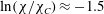 $\ln (\unicode[STIX]{x1D712}/\unicode[STIX]{x1D712}_{C})\approx -1.5$
. The low values of
$\ln (\unicode[STIX]{x1D712}/\unicode[STIX]{x1D712}_{C})\approx -1.5$
. The low values of
 $\unicode[STIX]{x1D712}$
on the
$\unicode[STIX]{x1D712}$
on the
 $\unicode[STIX]{x1D709}_{ST}$
surface are due to the small value of
$\unicode[STIX]{x1D709}_{ST}$
surface are due to the small value of
 $\unicode[STIX]{x1D709}_{ST}$
and the initial centreline
$\unicode[STIX]{x1D709}_{ST}$
and the initial centreline
 $\unicode[STIX]{x1D709}$
value of unity, causing the conditional
$\unicode[STIX]{x1D709}$
value of unity, causing the conditional
 $\unicode[STIX]{x1D709}$
profile to peak in very rich mixtures and become small near
$\unicode[STIX]{x1D709}$
profile to peak in very rich mixtures and become small near
 $\unicode[STIX]{x1D709}_{ST}$
(see figure 9). It is possible, that for the same nominal turbulent and chemical conditions but with a conditional
$\unicode[STIX]{x1D709}_{ST}$
(see figure 9). It is possible, that for the same nominal turbulent and chemical conditions but with a conditional
 $\unicode[STIX]{x1D712}$
profile that peaks near
$\unicode[STIX]{x1D712}$
profile that peaks near
 $\unicode[STIX]{x1D709}_{ST}$
, that the results presented here would differ greatly in terms of featuring: failed ignition kernels, local extinction of burning surface, reduced edge-flame speeds and enhanced flame folding.
$\unicode[STIX]{x1D709}_{ST}$
, that the results presented here would differ greatly in terms of featuring: failed ignition kernels, local extinction of burning surface, reduced edge-flame speeds and enhanced flame folding.

Figure 24. Joint PDF of the logarithm of dissipation rates with
 $S_{e}/s_{L}$
, its components
$S_{e}/s_{L}$
, its components
 $(S_{Y_{P}}/s_{L})/\sqrt{1-\boldsymbol{ k}^{2}}$
and
$(S_{Y_{P}}/s_{L})/\sqrt{1-\boldsymbol{ k}^{2}}$
and
 $(-\boldsymbol{k}S_{\unicode[STIX]{x1D709}}/s_{L})/\sqrt{1-\boldsymbol{ k}^{2}}$
and
$(-\boldsymbol{k}S_{\unicode[STIX]{x1D709}}/s_{L})/\sqrt{1-\boldsymbol{ k}^{2}}$
and
 $\boldsymbol{k}$
. The colour map shows the joint PDF information and the grey dashed line indicates the mean ordinate value, conditioned upon the abscissa value,
$\boldsymbol{k}$
. The colour map shows the joint PDF information and the grey dashed line indicates the mean ordinate value, conditioned upon the abscissa value,
 $\ln (\unicode[STIX]{x1D712})$
.
$\ln (\unicode[STIX]{x1D712})$
.
Regarding the correlations, for
 $\ln (\unicode[STIX]{x1D712}/\unicode[STIX]{x1D712}_{C})$
between
$\ln (\unicode[STIX]{x1D712}/\unicode[STIX]{x1D712}_{C})$
between
 $-5$
and
$-5$
and
 $-3.5$
, there is a positive correlation with
$-3.5$
, there is a positive correlation with
 $S_{e}$
, but for
$S_{e}$
, but for
 $\ln (\unicode[STIX]{x1D712}/\unicode[STIX]{x1D712}_{C})$
between
$\ln (\unicode[STIX]{x1D712}/\unicode[STIX]{x1D712}_{C})$
between
 $-3.5$
and 0.5 (the most probable range of values),
$-3.5$
and 0.5 (the most probable range of values),
 $S_{e}$
is negatively correlated. At very high
$S_{e}$
is negatively correlated. At very high
 $\unicode[STIX]{x1D712}$
values a slight increase in
$\unicode[STIX]{x1D712}$
values a slight increase in
 $S_{e}$
is observed. The conditional mean of
$S_{e}$
is observed. The conditional mean of
 $S_{e}$
peaks at approximately
$S_{e}$
peaks at approximately
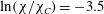 $\ln (\unicode[STIX]{x1D712}/\unicode[STIX]{x1D712}_{C})=-3.5$
and the marginal PDF in
$\ln (\unicode[STIX]{x1D712}/\unicode[STIX]{x1D712}_{C})=-3.5$
and the marginal PDF in
 $S_{e}$
space at this point is broad and skewed towards high values of
$S_{e}$
space at this point is broad and skewed towards high values of
 $S_{e}$
. The first component of the edge-flame speed,
$S_{e}$
. The first component of the edge-flame speed,
 $(S_{Y_{P}}/s_{L})/\sqrt{1-\boldsymbol{ k}^{2}}$
, is positive and higher in magnitude than
$(S_{Y_{P}}/s_{L})/\sqrt{1-\boldsymbol{ k}^{2}}$
, is positive and higher in magnitude than
 $S_{e}$
. At high levels of
$S_{e}$
. At high levels of
 $\ln (\unicode[STIX]{x1D712}/\unicode[STIX]{x1D712}_{C})$
, there is a strong, positive correlation with increasing
$\ln (\unicode[STIX]{x1D712}/\unicode[STIX]{x1D712}_{C})$
, there is a strong, positive correlation with increasing
 $\ln (\unicode[STIX]{x1D712}/\unicode[STIX]{x1D712}_{C})$
. The second component of
$\ln (\unicode[STIX]{x1D712}/\unicode[STIX]{x1D712}_{C})$
. The second component of
 $S_{e}$
,
$S_{e}$
,
 $(-\boldsymbol{k}S_{\unicode[STIX]{x1D709}}/s_{L})/\sqrt{1-\boldsymbol{ k}^{2}}$
, has a more narrow joint distribution. At low levels of dissipation, the magnitude of
$(-\boldsymbol{k}S_{\unicode[STIX]{x1D709}}/s_{L})/\sqrt{1-\boldsymbol{ k}^{2}}$
, has a more narrow joint distribution. At low levels of dissipation, the magnitude of
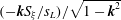 $(-\boldsymbol{k}S_{\unicode[STIX]{x1D709}}/s_{L})/\sqrt{1-\boldsymbol{ k}^{2}}$
is small and the most likely values are negative. At high levels of dissipation the speed decreases rapidly, balancing the rapid increase in the
$(-\boldsymbol{k}S_{\unicode[STIX]{x1D709}}/s_{L})/\sqrt{1-\boldsymbol{ k}^{2}}$
is small and the most likely values are negative. At high levels of dissipation the speed decreases rapidly, balancing the rapid increase in the
 $(S_{Y_{P}}/s_{L})/\sqrt{1-\boldsymbol{ k}^{2}}$
component. The results for
$(S_{Y_{P}}/s_{L})/\sqrt{1-\boldsymbol{ k}^{2}}$
component. The results for
 $k$
reveal a positive correlation between
$k$
reveal a positive correlation between
 $\unicode[STIX]{x1D712}$
and
$\unicode[STIX]{x1D712}$
and
 $k$
. The correlation is most pronounced for high values of
$k$
. The correlation is most pronounced for high values of
 $\unicode[STIX]{x1D712}$
where the joint PDF becomes narrow and rapidly approaches
$\unicode[STIX]{x1D712}$
where the joint PDF becomes narrow and rapidly approaches
 $k=1$
. The joint PDF for
$k=1$
. The joint PDF for
 $k$
explains the sharp ‘up tick’ and ‘down tick’ at high
$k$
explains the sharp ‘up tick’ and ‘down tick’ at high
 $\unicode[STIX]{x1D712}$
values for the components of
$\unicode[STIX]{x1D712}$
values for the components of
 $S_{e}$
. At lower
$S_{e}$
. At lower
 $\unicode[STIX]{x1D712}$
values the
$\unicode[STIX]{x1D712}$
values the
 $S_{e}/s_{L}$
statistics closely resemble those of the
$S_{e}/s_{L}$
statistics closely resemble those of the
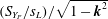 $(S_{Y_{P}}/s_{L})/\sqrt{1-\boldsymbol{ k}^{2}}$
component, with a near-uniform reduction due to the negative
$(S_{Y_{P}}/s_{L})/\sqrt{1-\boldsymbol{ k}^{2}}$
component, with a near-uniform reduction due to the negative
 $(-\boldsymbol{k}S_{\unicode[STIX]{x1D709}}/s_{L})/\sqrt{1-\boldsymbol{ k}^{2}}$
term.
$(-\boldsymbol{k}S_{\unicode[STIX]{x1D709}}/s_{L})/\sqrt{1-\boldsymbol{ k}^{2}}$
term.
The results indicate that the scalar dissipation rate has a non-monotonic impact on the edge-flame speed. For low values of
 $\unicode[STIX]{x1D712}$
, the edge-flame speed is slightly promoted by increasing
$\unicode[STIX]{x1D712}$
, the edge-flame speed is slightly promoted by increasing
 $\unicode[STIX]{x1D712}$
. This can be attributed to the increase in the
$\unicode[STIX]{x1D712}$
. This can be attributed to the increase in the
 $(S_{Y_{P}}/s_{L})/\sqrt{1-\boldsymbol{ k}^{2}}$
component. At intermediate values of
$(S_{Y_{P}}/s_{L})/\sqrt{1-\boldsymbol{ k}^{2}}$
component. At intermediate values of
 $\unicode[STIX]{x1D712}$
, both components of
$\unicode[STIX]{x1D712}$
, both components of
 $S_{e}$
are reduced with increasing
$S_{e}$
are reduced with increasing
 $\unicode[STIX]{x1D712}$
, causing a modest attenuation in
$\unicode[STIX]{x1D712}$
, causing a modest attenuation in
 $S_{e}$
. At very high
$S_{e}$
. At very high
 $\unicode[STIX]{x1D712}$
rates, the
$\unicode[STIX]{x1D712}$
rates, the
 $Y_{P}$
and
$Y_{P}$
and
 $\unicode[STIX]{x1D709}_{ST}$
surfaces become aligned, causing the components of
$\unicode[STIX]{x1D709}_{ST}$
surfaces become aligned, causing the components of
 $S_{e}$
to increase in magnitude rapidly and with opposite sign. Overall, the effect on
$S_{e}$
to increase in magnitude rapidly and with opposite sign. Overall, the effect on
 $S_{e}$
is a slight increase at very high
$S_{e}$
is a slight increase at very high
 $\unicode[STIX]{x1D712}$
values, with the caveat that the sample size at very high dissipate rates is small.
$\unicode[STIX]{x1D712}$
values, with the caveat that the sample size at very high dissipate rates is small.
Two observations are made with regard to the magnitude of
 $s_{e}/s_{L}$
. Firstly, the flow velocities near the stabilisation location in diesel flames are
$s_{e}/s_{L}$
. Firstly, the flow velocities near the stabilisation location in diesel flames are
 ${\approx}10~\text{m}~\text{s}^{-1}$
(Pei et al.
Reference Pei, Hawkes, Bolla, Kook, Goldin, Yang, Pope and Som2016). This is only 2–3 times the observed (dimensional) local
${\approx}10~\text{m}~\text{s}^{-1}$
(Pei et al.
Reference Pei, Hawkes, Bolla, Kook, Goldin, Yang, Pope and Som2016). This is only 2–3 times the observed (dimensional) local
 $s_{e}$
in this DNS, and the turbulence experienced at diesel engine conditions could potentially increase the net overall propagation speeds over and above the local propagation speed by wrinkling of the edge-flame structure, similar to how in premixed turbulent flames the net burning velocity is much larger than
$s_{e}$
in this DNS, and the turbulence experienced at diesel engine conditions could potentially increase the net overall propagation speeds over and above the local propagation speed by wrinkling of the edge-flame structure, similar to how in premixed turbulent flames the net burning velocity is much larger than
 $s_{L}$
.
$s_{L}$
.

Figure 25. Left
 $y$
-axis: non-dimensional speeds for
$y$
-axis: non-dimensional speeds for
 $s_{L}/s_{L,0}$
(circles),
$s_{L}/s_{L,0}$
(circles),
 $\sqrt{\unicode[STIX]{x1D70C}_{u}/\unicode[STIX]{x1D70C}_{b}}s_{L}/s_{L,0}$
(pluses) and
$\sqrt{\unicode[STIX]{x1D70C}_{u}/\unicode[STIX]{x1D70C}_{b}}s_{L}/s_{L,0}$
(pluses) and
 $\unicode[STIX]{x1D70C}_{u}/\unicode[STIX]{x1D70C}_{f}s_{L}/s_{L,0}$
(triangles) with respect to the ignition progress of the reactant mixture. Right
$\unicode[STIX]{x1D70C}_{u}/\unicode[STIX]{x1D70C}_{f}s_{L}/s_{L,0}$
(triangles) with respect to the ignition progress of the reactant mixture. Right
 $y$
-axis: PDF for the ignition progress measured
$y$
-axis: PDF for the ignition progress measured
 $2\times \unicode[STIX]{x1D6FF}_{L}$
ahead of the edge flame on the
$2\times \unicode[STIX]{x1D6FF}_{L}$
ahead of the edge flame on the
 $\unicode[STIX]{x1D709}_{ST}$
isosurface.
$\unicode[STIX]{x1D709}_{ST}$
isosurface.
The second observation is that the non-dimensionalised speed
 $s_{e}/s_{L}$
exceeds unity. This is expected for both hydrodynamic reasons due to flow expansion (Ruetsch, Vervisch & Liñán Reference Ruetsch, Vervisch and Liñán1995; Im & Chen Reference Im and Chen1999) and thermochemical reasons due to enhanced flame propagation into a partially reacted mixture ahead of the flames (Minamoto & Chen Reference Minamoto and Chen2016). Flow expansion occurs across a premixed flame due to the temperature increase from combustion. For this reason, displacement speeds are often weighted by the ratio of the local density at the flame,
$s_{e}/s_{L}$
exceeds unity. This is expected for both hydrodynamic reasons due to flow expansion (Ruetsch, Vervisch & Liñán Reference Ruetsch, Vervisch and Liñán1995; Im & Chen Reference Im and Chen1999) and thermochemical reasons due to enhanced flame propagation into a partially reacted mixture ahead of the flames (Minamoto & Chen Reference Minamoto and Chen2016). Flow expansion occurs across a premixed flame due to the temperature increase from combustion. For this reason, displacement speeds are often weighted by the ratio of the local density at the flame,
 $\unicode[STIX]{x1D70C}_{f}$
, to the unburnt density,
$\unicode[STIX]{x1D70C}_{f}$
, to the unburnt density,
 $\unicode[STIX]{x1D70C}_{u}$
(Echekki & Chen Reference Echekki and Chen1998; Im & Chen Reference Im and Chen1999). Here, this equates to the expression
$\unicode[STIX]{x1D70C}_{u}$
(Echekki & Chen Reference Echekki and Chen1998; Im & Chen Reference Im and Chen1999). Here, this equates to the expression
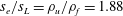 $s_{e}/s_{L}=\unicode[STIX]{x1D70C}_{u}/\unicode[STIX]{x1D70C}_{f}=1.88$
. Alternatively, the deviation between
$s_{e}/s_{L}=\unicode[STIX]{x1D70C}_{u}/\unicode[STIX]{x1D70C}_{f}=1.88$
. Alternatively, the deviation between
 $s_{L}$
and
$s_{L}$
and
 $s_{e}$
can be explained by the divergence of streamlines across the edge flame (Ruetsch et al.
Reference Ruetsch, Vervisch and Liñán1995). The streamline divergence causes flow deceleration just ahead of the triple point, and so displacement speed measurements made at this location underestimate the true edge-flame speed. Taking this effect into account yields a correction factor of
$s_{e}$
can be explained by the divergence of streamlines across the edge flame (Ruetsch et al.
Reference Ruetsch, Vervisch and Liñán1995). The streamline divergence causes flow deceleration just ahead of the triple point, and so displacement speed measurements made at this location underestimate the true edge-flame speed. Taking this effect into account yields a correction factor of
 $s_{e}/s_{L}=\sqrt{\unicode[STIX]{x1D70C}_{u}/\unicode[STIX]{x1D70C}_{b}}=1.47$
, where
$s_{e}/s_{L}=\sqrt{\unicode[STIX]{x1D70C}_{u}/\unicode[STIX]{x1D70C}_{b}}=1.47$
, where
 $\unicode[STIX]{x1D70C}_{b}$
is the burnt density. Since the displacement speeds here are evaluated where the HRR is maximum on the product side, and not on the reactant side of the triple point where the streamline divergence is greatest, it is argued that the relevant correction factor here is
$\unicode[STIX]{x1D70C}_{b}$
is the burnt density. Since the displacement speeds here are evaluated where the HRR is maximum on the product side, and not on the reactant side of the triple point where the streamline divergence is greatest, it is argued that the relevant correction factor here is
 $\unicode[STIX]{x1D70C}_{u}/\unicode[STIX]{x1D70C}_{f}=1.88$
. This factor is insufficient to account for the values of
$\unicode[STIX]{x1D70C}_{u}/\unicode[STIX]{x1D70C}_{f}=1.88$
. This factor is insufficient to account for the values of
 $s_{e}/s_{L}$
here, which mostly lie between 1.8 and 3.5. Another correction due to the partially reacted mixture ahead of the flame is required. As discussed by Minamoto & Chen (Reference Minamoto and Chen2016), the value of
$s_{e}/s_{L}$
here, which mostly lie between 1.8 and 3.5. Another correction due to the partially reacted mixture ahead of the flame is required. As discussed by Minamoto & Chen (Reference Minamoto and Chen2016), the value of
 $s_{L}$
for autoignitive conditions is dependent upon the state of the reactant mixture, since pre-ignition reactions due to LTC may occur ahead of the premixed flame. In order to evaluate this effect, figure 25 presents the response of non-dimensionalised flame speeds to the upstream ignition progress, measured by
$s_{L}$
for autoignitive conditions is dependent upon the state of the reactant mixture, since pre-ignition reactions due to LTC may occur ahead of the premixed flame. In order to evaluate this effect, figure 25 presents the response of non-dimensionalised flame speeds to the upstream ignition progress, measured by
 $Y_{P}/Y_{P,b}$
, where
$Y_{P}/Y_{P,b}$
, where
 $Y_{P,b}$
is the burnt value of
$Y_{P,b}$
is the burnt value of
 $Y_{P}$
and the laminar flame speed at zero progress,
$Y_{P}$
and the laminar flame speed at zero progress,
 $s_{L,0}$
, is used to non-dimensional all values. Also plotted on figure 25 is the PDF of ignition progress upstream of the edge-flame location. The PDF is composed of all samples on the unburnt
$s_{L,0}$
, is used to non-dimensional all values. Also plotted on figure 25 is the PDF of ignition progress upstream of the edge-flame location. The PDF is composed of all samples on the unburnt
 $\unicode[STIX]{x1D709}_{ST}$
isosurface during ignition that are
$\unicode[STIX]{x1D709}_{ST}$
isosurface during ignition that are
 $2\times \unicode[STIX]{x1D6FF}_{L}$
(Sensitivity to this distance was assessed for values between 1.5 and
$2\times \unicode[STIX]{x1D6FF}_{L}$
(Sensitivity to this distance was assessed for values between 1.5 and
 $3\times \unicode[STIX]{x1D6FF}_{L}$
and the result was not strongly affected as the spatial gradient of ignition progress sufficiently far from the edge flame was small.) ahead of an edge-flame location. As expected,
$3\times \unicode[STIX]{x1D6FF}_{L}$
and the result was not strongly affected as the spatial gradient of ignition progress sufficiently far from the edge flame was small.) ahead of an edge-flame location. As expected,
 $s_{L}/s_{L,0}$
increases with ignition progress but by itself does not account for the discrepancy with the observed values of
$s_{L}/s_{L,0}$
increases with ignition progress but by itself does not account for the discrepancy with the observed values of
 $s_{e}/s_{L}$
. The correction factor
$s_{e}/s_{L}$
. The correction factor
 $\sqrt{\unicode[STIX]{x1D70C}_{u}/\unicode[STIX]{x1D70C}_{b}}s_{L}/s_{L,0}$
is also lower than most observed values of
$\sqrt{\unicode[STIX]{x1D70C}_{u}/\unicode[STIX]{x1D70C}_{b}}s_{L}/s_{L,0}$
is also lower than most observed values of
 $s_{e}/s_{L}$
. However, the correction factor due to dilatation at the flame location,
$s_{e}/s_{L}$
. However, the correction factor due to dilatation at the flame location,
 $\unicode[STIX]{x1D70C}_{u}/\unicode[STIX]{x1D70C}_{f}s_{L}/s_{L,0}$
, is close to the range of likely values of
$\unicode[STIX]{x1D70C}_{u}/\unicode[STIX]{x1D70C}_{f}s_{L}/s_{L,0}$
, is close to the range of likely values of
 $s_{e}/s_{L}$
as shown in figure 24. Even with this correction, there is still a slight discrepancy between
$s_{e}/s_{L}$
as shown in figure 24. Even with this correction, there is still a slight discrepancy between
 $s_{e}/s_{L}$
(higher) and
$s_{e}/s_{L}$
(higher) and
 $\unicode[STIX]{x1D70C}_{u}/\unicode[STIX]{x1D70C}_{f}s_{L}/s_{L,0}$
(lower) for the likely range of ignition progress values upstream of the flame. This may be explained by: (i) non-edge-flame ignition modes introducing a positive bias to the
$\unicode[STIX]{x1D70C}_{u}/\unicode[STIX]{x1D70C}_{f}s_{L}/s_{L,0}$
(lower) for the likely range of ignition progress values upstream of the flame. This may be explained by: (i) non-edge-flame ignition modes introducing a positive bias to the
 $s_{e}/s_{L}$
statistics, which do not distinguish between ignition modes; (ii) turbulent enhancement of
$s_{e}/s_{L}$
statistics, which do not distinguish between ignition modes; (ii) turbulent enhancement of
 $s_{e}/s_{L}$
, via wrinkling of the edge-flame front; (iii) the definition of
$s_{e}/s_{L}$
, via wrinkling of the edge-flame front; (iii) the definition of
 $s_{L}$
used here (see § 2.3) may provide an underestimate of the true laminar reference speed for a given reactant composition. Despite the slight discrepancy, this result provides evidence that the ignition of the
$s_{L}$
used here (see § 2.3) may provide an underestimate of the true laminar reference speed for a given reactant composition. Despite the slight discrepancy, this result provides evidence that the ignition of the
 $\unicode[STIX]{x1D709}_{ST}$
isosurface is primarily explained by autoignition-assisted edge-flame propagation, as opposed to the expansion of independent autoignition kernels from rich mixtures engulfing the
$\unicode[STIX]{x1D709}_{ST}$
isosurface is primarily explained by autoignition-assisted edge-flame propagation, as opposed to the expansion of independent autoignition kernels from rich mixtures engulfing the
 $\unicode[STIX]{x1D709}_{ST}$
isosurface, or through turbulent flame folding, as these ignition modes could in principle take a wider range of values and are not constrained by the physical arguments considered here. This interpretation is also consistent with a visual inspection of the
$\unicode[STIX]{x1D709}_{ST}$
isosurface, or through turbulent flame folding, as these ignition modes could in principle take a wider range of values and are not constrained by the physical arguments considered here. This interpretation is also consistent with a visual inspection of the
 $\unicode[STIX]{x1D709}_{ST}$
isosurface over time. For example, figure 7 showed the evolution of the state of the
$\unicode[STIX]{x1D709}_{ST}$
isosurface over time. For example, figure 7 showed the evolution of the state of the
 $\unicode[STIX]{x1D709}_{MR}$
isosurface in terms of burning and non-burning regions. Those images (and time resolved images not shown here) support the notion that the independent burning ‘spots’ due to the expanding ignition kernels are responsible for the initiation of ignition of the
$\unicode[STIX]{x1D709}_{MR}$
isosurface in terms of burning and non-burning regions. Those images (and time resolved images not shown here) support the notion that the independent burning ‘spots’ due to the expanding ignition kernels are responsible for the initiation of ignition of the
 $\unicode[STIX]{x1D709}_{ST}$
isosurface, but that it is edge-flame propagation that consumes the majority of the
$\unicode[STIX]{x1D709}_{ST}$
isosurface, but that it is edge-flame propagation that consumes the majority of the
 $\unicode[STIX]{x1D709}_{ST}$
isosurface.
$\unicode[STIX]{x1D709}_{ST}$
isosurface.

Figure 26. Ensemble mean of alignment factor
 $k$
, conditioned upon
$k$
, conditioned upon
 $\unicode[STIX]{x1D712}$
and
$\unicode[STIX]{x1D712}$
and
 $S_{e}$
. Superimposed in white is the joint PDF of
$S_{e}$
. Superimposed in white is the joint PDF of
 $\unicode[STIX]{x1D712}$
and
$\unicode[STIX]{x1D712}$
and
 $S_{e}$
and superimposed in black is the mean value of
$S_{e}$
and superimposed in black is the mean value of
 $S_{e}$
conditioned on
$S_{e}$
conditioned on
 $\unicode[STIX]{x1D712}$
, as presented in figure 24.
$\unicode[STIX]{x1D712}$
, as presented in figure 24.
In order to provide further evidence for the relative contribution of ignition modes, the ensemble-averaged alignment factor
 $k$
, doubly conditioned upon
$k$
, doubly conditioned upon
 $S_{\unicode[STIX]{x1D709}}$
and
$S_{\unicode[STIX]{x1D709}}$
and
 $\unicode[STIX]{x1D712}$
, is presented alongside the joint PDF of
$\unicode[STIX]{x1D712}$
, is presented alongside the joint PDF of
 $S_{\unicode[STIX]{x1D709}}$
and
$S_{\unicode[STIX]{x1D709}}$
and
 $\unicode[STIX]{x1D712}$
in figure 26. For
$\unicode[STIX]{x1D712}$
in figure 26. For
 $\ln (\unicode[STIX]{x1D712}/\unicode[STIX]{x1D712}_{C})<-0.5$
and
$\ln (\unicode[STIX]{x1D712}/\unicode[STIX]{x1D712}_{C})<-0.5$
and
 $S_{e}/s_{L}<4.5$
, the alignment factor takes a low to intermediate value, consistent with an edge-flame propagation ignition mode (Hawkes et al.
Reference Hawkes, Sankaran and Chen2008). This corresponds to the most probable region of the joint PDF where the
$S_{e}/s_{L}<4.5$
, the alignment factor takes a low to intermediate value, consistent with an edge-flame propagation ignition mode (Hawkes et al.
Reference Hawkes, Sankaran and Chen2008). This corresponds to the most probable region of the joint PDF where the
 $s_{e}/s_{L}$
values correspond to those predicted by the
$s_{e}/s_{L}$
values correspond to those predicted by the
 $\unicode[STIX]{x1D70C}_{u}/\unicode[STIX]{x1D70C}_{f}s_{L}/s_{L,0}$
scaling, which provides further evidence that autoignition-assisted edge-flame propagation is the dominant mode of ignition in this case. These edge flames are therefore akin to the hybrid premixed/autoignitive edge flames previously observed with detailed dimethyl-ether chemistry in two dimensions (Krisman et al.
Reference Krisman, Hawkes, Talei, Bhagatwala and Chen2015) and three dimensions (Minamoto & Chen Reference Minamoto and Chen2016) DNS.
$\unicode[STIX]{x1D70C}_{u}/\unicode[STIX]{x1D70C}_{f}s_{L}/s_{L,0}$
scaling, which provides further evidence that autoignition-assisted edge-flame propagation is the dominant mode of ignition in this case. These edge flames are therefore akin to the hybrid premixed/autoignitive edge flames previously observed with detailed dimethyl-ether chemistry in two dimensions (Krisman et al.
Reference Krisman, Hawkes, Talei, Bhagatwala and Chen2015) and three dimensions (Minamoto & Chen Reference Minamoto and Chen2016) DNS.
Two regions of high
 $\boldsymbol{k}$
value and low probability are also observed. The first region occurs for
$\boldsymbol{k}$
value and low probability are also observed. The first region occurs for
 $\ln (\unicode[STIX]{x1D712}/\unicode[STIX]{x1D712}_{C})>-0.5$
. This region may be attributed to either a flame-folding mode, or an autoignition mode as both are associated with high values of
$\ln (\unicode[STIX]{x1D712}/\unicode[STIX]{x1D712}_{C})>-0.5$
. This region may be attributed to either a flame-folding mode, or an autoignition mode as both are associated with high values of
 $k$
and
$k$
and
 $\unicode[STIX]{x1D712}$
. Flame folding requires a strong interaction between the turbulent field and the stoichiometric surface. However, due to the low value of
$\unicode[STIX]{x1D712}$
. Flame folding requires a strong interaction between the turbulent field and the stoichiometric surface. However, due to the low value of
 $\unicode[STIX]{x1D709}_{ST}$
in the present case, the
$\unicode[STIX]{x1D709}_{ST}$
in the present case, the
 $\unicode[STIX]{x1D709}_{ST}$
isosurface resides at the jet periphery and is only moderately distorted by the turbulent jet. This suggests that flame folding in unlikely to be a significant ignition mode, which is supported by visual inspection of the burning surface evolution. For this reason, autoignition rather than flame folding is proposed to be responsible for the high
$\unicode[STIX]{x1D709}_{ST}$
isosurface resides at the jet periphery and is only moderately distorted by the turbulent jet. This suggests that flame folding in unlikely to be a significant ignition mode, which is supported by visual inspection of the burning surface evolution. For this reason, autoignition rather than flame folding is proposed to be responsible for the high
 $\unicode[STIX]{x1D712}$
, high
$\unicode[STIX]{x1D712}$
, high
 $\boldsymbol{k}$
, but low probability region of the joint PDF.
$\boldsymbol{k}$
, but low probability region of the joint PDF.
The second region occurs for
 $S_{e}/s_{L}>4$
. This region coincides with an extremely low probability region of the joint PDF at intermediate
$S_{e}/s_{L}>4$
. This region coincides with an extremely low probability region of the joint PDF at intermediate
 $\unicode[STIX]{x1D712}$
values and very high edge-flame speeds. Visual inspection of the domain shows that multiple edge-flame collisions occurs as a larger proportion of the stoichiometric surface reaches a burning state. As shown in figure 6, where the edge flames meet, the rich premixed branches can collide before the triple points on the
$\unicode[STIX]{x1D712}$
values and very high edge-flame speeds. Visual inspection of the domain shows that multiple edge-flame collisions occurs as a larger proportion of the stoichiometric surface reaches a burning state. As shown in figure 6, where the edge flames meet, the rich premixed branches can collide before the triple points on the
 $\unicode[STIX]{x1D709}_{ST}$
surface do. This causes the
$\unicode[STIX]{x1D709}_{ST}$
surface do. This causes the
 $Y_{P}$
surface to become aligned with the
$Y_{P}$
surface to become aligned with the
 $\unicode[STIX]{x1D709}_{ST}$
surface and therefore results in a high value of
$\unicode[STIX]{x1D709}_{ST}$
surface and therefore results in a high value of
 $k$
, but not necessarily a larger value of
$k$
, but not necessarily a larger value of
 $\unicode[STIX]{x1D712}$
. Visual inspection also suggests that the edge-flame collisions are associated with an acceleration of the ignition of the
$\unicode[STIX]{x1D712}$
. Visual inspection also suggests that the edge-flame collisions are associated with an acceleration of the ignition of the
 $\unicode[STIX]{x1D709}_{ST}$
surface due to vanishing scalar gradients during the collision. Based upon this evidence, it is proposed that edge-flame collisions are responsible for the high
$\unicode[STIX]{x1D709}_{ST}$
surface due to vanishing scalar gradients during the collision. Based upon this evidence, it is proposed that edge-flame collisions are responsible for the high
 $S_{e}$
, high
$S_{e}$
, high
 $k$
, but low probability region of the joint PDF. This ignition mode therefore introduces a positive bias to the mean values of
$k$
, but low probability region of the joint PDF. This ignition mode therefore introduces a positive bias to the mean values of
 $s_{e}/s_{L}$
reported here and may explain why some samples have
$s_{e}/s_{L}$
reported here and may explain why some samples have
 $s_{e}/s_{L}$
larger than expected from the
$s_{e}/s_{L}$
larger than expected from the
 $\unicode[STIX]{x1D70C}_{u}/\unicode[STIX]{x1D70C}_{f}s_{L}/s_{L,0}$
scaling argument.
$\unicode[STIX]{x1D70C}_{u}/\unicode[STIX]{x1D70C}_{f}s_{L}/s_{L,0}$
scaling argument.
4 Conclusions
A direct numerical simulation was performed of an igniting, three-dimensional, temporally evolving n-heptane/air slot jet at 40 atm. A global chemical mechanism was used for computational affordability while retaining the two-stage autoignition behaviour of diesel fuel. Overall, a two-stage autoignition event was observed that transitioned to edge-flame propagation.
The main findings of the study are summarised as follows.
-
(i) The first stage of autoignition developed in rich mixtures and moves up the mixture-fraction gradient. However, the peak conditional scalar dissipation rates are sufficient to inhibit the intensity of the conditionally averaged LTC. The peak conditional scalar dissipation rates occurred due to the development of shear-driven turbulence during the initial transition of the mean laminar jet profile to fully developed turbulence. As dissipation rates relaxed, the LTC recovers and leads to the second stage of autoignition.
-
(ii) The second stage of autoignition occurs as a distributed (in physical and composition space), sequential event comprising multiple ignition kernels. The ignition kernels form over a range of mixture fractions, both lower and higher than the homogeneous most reactive mixture fraction.
-
(iii) A topological analysis during ignition revealed that the LTC and onset of HTC ignition occurs preferentially in vortically dominated regions of the jet. After the onset of HTC ignition, the strongest burning occurs in strain-dominated topologies associated with premixed flame fronts.
-
(iv) The formation of ignition kernels in rich mixtures and at low scalar dissipation rates and within vortical topology types is consistent with a previous autoignition DNS in isotropic turbulence using a similar chemical mechanism (Sreedhara & Lakshmisha Reference Sreedhara and Lakshmisha2002). In the present results, the exact location of the ignition kernel formation is available, in addition to the Lagrangian history of each igniting fluid element. Analysis of the kernel histories reveal that all ignition kernels pass through a period of intense mixing followed by a rapid decrease in mixing rates and a convergence to mixture fractions corresponding to short homogeneous ignition delay times. The timing of kernel mixing is a parameter that is positively correlated with the formation of the ignition kernel.
-
(v) An analysis of edge-flame speeds with respect to scalar dissipation rates was conducted. Overall, the edge-flame speed is negatively correlated with dissipation rates, which is consistent with studies of edge-flame extinction at atmospheric conditions.
-
(vi) The edge-flame analysis was also used to evaluate the relative contributions of ignition modes on the
 $\unicode[STIX]{x1D709}_{ST}$
isosurface. The following observations were made:
$\unicode[STIX]{x1D709}_{ST}$
isosurface. The following observations were made:-
(1) The non-dimensionalised edge-flame speeds are in good agreement with values predicted by the expression
$\unicode[STIX]{x1D70C}_{u}/\unicode[STIX]{x1D70C}_{f}s_{L}/s_{L,0}$
, which assumes that the ignition occurs via edge-flame propagation, and which takes into account the local dilatation due to the premixed flame (
$\unicode[STIX]{x1D70C}_{u}/\unicode[STIX]{x1D70C}_{f}$
) and the laminar flame speed enhancement due to the autoignitive conditions ahead of the flame (
$s_{L}/s_{L,0}$
). -
(2) The edge-flame speed, which has components due to both the displacement speed of a mixture-fraction isosurface and a product mass fraction isosurface, is observed to be mostly controlled by the movement of the product mass fraction surface. If autoignition is dominant, greater flame motion in the mixture-fraction normal direction would be expected at the stoichiometric location since ignition occurs first in richer mixtures.
-
(3) The isosurfaces are poorly aligned at most locations, which is expected for edge-flame propagation and not for autoignition or flame folding.
These observations strongly suggest that the ignition of the
$\unicode[STIX]{x1D709}_{ST}$
isosurface, although initiated by isolated autoignition kernels, is predominantly due to edge-flame propagation that is enhanced by the partially reacted mixture ahead of the flame. This is therefore consistent with the hybrid autoignitive/premixed polybrachial edge flames that have been observed for laminar (Krisman et al.
Reference Krisman, Hawkes, Talei, Bhagatwala and Chen2015) and turbulent (Minamoto & Chen Reference Minamoto and Chen2016) dimethyl-ether lifted flames with detailed chemistry. -


The conclusions of this study may be affected by case-specific choices such as: (1) the global chemical mechanism, that would differ in particular in terms of the autoignition response to scalar dissipation rates compared to a detailed chemical mechanism; (2) the peak mixture fraction of the jet and the stoichiometric mixture-fraction values, which determines the location of the ignition kernels and edge flames with respect to the turbulence intensity and scalar dissipation profiles, and may therefore influence the ignition/extinction behaviour; and (3) the oxidiser temperature and
 $\text{O}_{2}$
concentration, which for a given pressure influences the location in mixture-fraction space and the time scales of the first and second stages of autoignition and the laminar flame speed.
$\text{O}_{2}$
concentration, which for a given pressure influences the location in mixture-fraction space and the time scales of the first and second stages of autoignition and the laminar flame speed.
Acknowledgements
This work was supported by the Australian Research Council. The work at Sandia National Laboratories was supported by the US Department of Energy, Office of Basic Energy Sciences, Division of Chemical Sciences, Geosciences, and Biosciences. Sandia National Laboratories is a multimission laboratory managed and operated by National Technology and Engineering Solutions of Sandia, LLC., a wholly owned subsidiary of Honeywell International, Inc., for the US Department of Energys National Nuclear Security Administration under contract DE-NA-0003525. This research used resources of the National Energy Research Computing Center (NERSC) which is supported by the Office of Science of the US DOE under contract no. DE-AC03-76SF00098. The research was also supported by computational resources on the Australian NCI National Facility through the National Computational Merit Allocation Scheme and Intersect Australia partner share and by resources at the Pawsey Supercomputing Centre.


