2.1 Pore-scale model

Instead of a full Navier–Stokes approach as is common for pore-scale simulations (see figure 2 a), the model adopts a micro-continuum formulation, whereby an arbitrary cutoff length is introduced and all the information regarding the solid structure below this length scale are filtered and modelled as a porous medium. Mathematically, this cutoff length is associated with a control volume, $V$ , that corresponds to a cell of the computational grid, and all the variables of the system are averaged over $V$ . The control volumes that contain void only, also called clear fluid regions or free zones, and those that contain solid are differentiated by $\unicode[STIX]{x1D700}_{f}$ , which is the volume fraction of void space within a control volume. It is defined as a field with different values all over the domain that range from 0 to 1. This filtering is illustrated in figure 2(b,c). The free zone is characterized by $\unicode[STIX]{x1D700}_{f}=1$ , whereby the flow is governed by Navier–Stokes equations in these areas. For intermediate values, $0<\unicode[STIX]{x1D700}_{f}<1$ , there are solid obstacles in the control volume, and the flow is governed by Darcy’s law. When $\unicode[STIX]{x1D700}_{f}=0$ , the control volume contains solid only, and there is no flow. Actually, to make the governing equations described below valid all over the computational domain, i.e. in the free and the solid regions, we assume that the cells describing solid regions always contain a tiny porosity, $\unicode[STIX]{x1D700}_{f}=0\equiv 0.001$ . Different from other micro-continuum models proposed to simulate core-scale phenomena (Liu et al. Reference Liu, Ormond, Bartko, Ying and Ortoleva1997; Ormond & Ortoleva Reference Ormond and Ortoleva2000; Golfier et al. Reference Golfier, Zarcone, Bazin, Lenormand, Lasseux and Quintard2002; Scheibe et al. Reference Scheibe, Perkins, Richmond, McKinley, Romero-Gomez, Oostrom, Wietsma, Serkowski and Zachara2015; Soulaine & Tchelepi Reference Soulaine and Tchelepi2016a ), here we use a DBS formulation to simulate the pore-scale physics. So, only the bounding values $\unicode[STIX]{x1D700}_{f}=1$ and $\unicode[STIX]{x1D700}_{f}=0$ are used to describe the porous structure at the pore scale. The intermediate values of void (or volume of solid) describe the interface between fluid and solid (see figure 2 c). The interface is not necessarily sharp and can be spread over several cells. So, this model belongs to the family of the diffuse interface models. Note that by definition, the relation

where $\unicode[STIX]{x1D700}_{s}$ is the volume fraction of solid, and $\unicode[STIX]{x1D700}_{f}$ the volume fraction of void, is always valid.

Likewise, the other variables of the system are defined as averaged quantities over the control volume (Whitaker Reference Whitaker1999). The pressure and acid mass fraction are intrinsic phase averages, $\bar{p}_{f}=(1/V_{f})\int _{V_{f}}p_{f}\,\text{d}V$ and $\bar{\unicode[STIX]{x1D714}}_{f,A}=(1/V_{f})\int _{V_{f}}\unicode[STIX]{x1D714}_{f,A}\,\text{d}V$ respectively, where $V_{f}$ is the volume occupied by the fluid in the control volume and the velocity is defined as a superficial average, $\bar{\boldsymbol{v}}_{f}=(1/V)\int _{V_{f}}\boldsymbol{v}_{f}\,\text{d}V$ , in agreement with Darcy’s law.

The flow model arises from the integration of the Navier–Stokes momentum equation over a control volume in the presence of solid material (Vafai & Tien Reference Vafai and Tien1981, Reference Vafai and Tien1982; Hsu & Cheng Reference Hsu and Cheng1990; Bousquet-Melou et al. Reference Bousquet-Melou, Goyeau, Quintard, Fichot and Gobin2002). The averaging process results in a single equation that holds in both the free flow and the porous medium domains. We have,

where the locally averaged pressure, $\bar{p}_{f}$ , and velocity field, $\bar{\boldsymbol{v}}_{f}$ , are the unknowns of the system. This equation is an extension of the original Darcy–Brinkman–Stokes equation (Brinkman Reference Brinkman1947) with inertia in the free zone and fluid/solid mass transfer described by the terms on the left-hand side. The two first terms on the right-hand side are the pressure gradient and the diffusive viscous contribution. The last term of the right-hand side of (2.2) represents the momentum exchange term between the fluid and the solid phase, i.e. the Darcy resistance term. It vanishes in the free zone, so that (2.2) degenerates to the Navier–Stokes equations. This drag term is dominant in the solid region so that the velocity is reduced to almost zero in this region. For low values of $k$ , i.e. at least four orders of magnitude below the permeability of the porous structure described by $\unicode[STIX]{x1D700}_{f}$ , it forces a no-slip boundary condition at the fluid/solid interface (Angot, Bruneau & Fabrie Reference Angot, Bruneau and Fabrie1999; Khadra et al. Reference Khadra, Angot, Parneix and Caltagirone2000; Soulaine & Tchelepi Reference Soulaine and Tchelepi2016a ).

During the dissolution process, the solid morphology evolves with chemical reactions at the mineral surfaces. To simplify the system, we consider one mineral only. Hence, the solid volume fraction in a control volume, $\unicode[STIX]{x1D700}_{s}$ , is an unknown of the system, and its evolution is governed by the mass balance equation

where $\unicode[STIX]{x1D70C}_{s}$ is the solid density and ${\dot{m}}$ is the rate of fluid/solid mass transfer. The latter has a non-zero value only at the fluid/solid interface. All the dissolved mass goes into the fluid phase, and the continuity equation for the fluid phase reads

where $\unicode[STIX]{x1D70C}_{f}$ is the fluid density. In this study, $\unicode[STIX]{x1D70C}_{f}$ is considered constant and independent of the fluid composition.

The solid is dissolved by an acid denoted $A$ . Because $A$ is the only species in the fluid phase that reacts with the solid phase, it is the only concentration in the fluid mixture solved in this model. The mass balance equation averaged over the control volume is

where $D_{A}^{\ast }$ denotes the effective diffusivity of species $A$ into the fluid mixture, and ${\dot{m}}_{A}$ is the rate of the chemical reaction of $A$ with the solid minerals. As for ${\dot{m}}$ , this term is non-zero only in the presence of solid minerals. To account for tortuosity in the cell matrix, the effective diffusivity is $\unicode[STIX]{x1D700}_{f}D_{A}^{\ast }=\unicode[STIX]{x1D700}_{f}^{2}D_{A}$ , where $D_{A}$ is the molecular diffusivity of the acid into the fluid mixture (Wakao & Smith Reference Wakao and Smith1962). Note that in the free zone, $\unicode[STIX]{x1D700}_{f}=1$ , and (2.5) degenerates to the classic advection–diffusion equation.

The mathematical problem formed by (2.2)–(2.5) is valid over the entire Eulerian grid whether the cell contains solid, or void. Importantly, in the clear fluid region, all the equations degenerate to the standard conservation laws of fluid mechanics. In the solid regions, the drag force term drops the velocity value to near zero, which enforces a no-slip boundary condition at the fluid/solid interface. During the dissolution process, the interface moves, and the local permeability field, $k$ , has to be updated according to the solid distribution in the computational grid. A Kozeny–Carman relation

is used here to estimate the local permeability as a function of porosity. Indeed, a Kozeny–Carman permeability–porosity relationship allows (2.2) to switch asymptotically from the continuum behaviour, where Darcian friction is dominant, to the Navier–Stokes pure fluid behaviour according to the cell porosity values: in the free zones, $\unicode[STIX]{x1D700}_{f}=1$ , and then $k^{-1}=0$ . In this equation, $k_{0}^{-1}$ is an input parameter that needs to be small enough. We have found that at least four orders of magnitude below the permeability of the sample are necessary to ensure the no-slip boundary condition.

The last ingredient of the model concerns the formulation of the mass exchange terms, ${\dot{m}}$ and ${\dot{m}}_{A}$ . First, the rate of dissolved mass is obtained from a simple mass balance

where $\unicode[STIX]{x1D6FD}$ is a stoichiometric coefficient. To calculate, ${\dot{m}}_{A}$ , we consider a first-order reaction rate, so the acid boundary condition at the solid surface is formulated as

where $\boldsymbol{n}_{fs}$ is the normal at the fluid/solid interface, $\boldsymbol{w}$ is the receding velocity of this interface due to the surface chemical reaction and $r$ is the reaction rate constant. A mass balance gives $\boldsymbol{n}_{fs}\boldsymbol{\cdot }\boldsymbol{w}=-r(\unicode[STIX]{x1D70C}_{f}/\unicode[STIX]{x1D70C}_{s})\unicode[STIX]{x1D6FD}\unicode[STIX]{x1D714}_{f,A}$ . The model presented in this paper has a micro-continuum formulation, which means that the flux boundary condition, equation (2.8), is not imposed directly at the edge of the computational grid, but instead is imposed as an immersed boundary condition. This is achieved by integrating (2.8) over a control volume; hence, the flux can be formulated as

where $a_{v}$ is the effective surface area in one cell of the Eulerian grid. To obtain (2.9), the spatial variations of the concentration inside a control volume are neglected and $\unicode[STIX]{x1D714}_{f,A}\approx \bar{\unicode[STIX]{x1D714}}_{f,A}$ . This assumption corresponds to the discretization error. Because we use a micro-continuum formulation for pore-scale simulation, there is a sharp transition between the clear fluid region and the solid region (see figure 2 c). Hence, the surface area per control volume is $a_{v}=\Vert \unicode[STIX]{x1D735}\unicode[STIX]{x1D700}_{f}\Vert$ . This relationship between the specific area and the porosity gradient arises from the volume averaging theorem, $-\unicode[STIX]{x1D735}\unicode[STIX]{x1D700}_{f}=(1/V)\int _{A_{fs}}\boldsymbol{n}_{fs}\,\text{d}A$ , that relates the gradient of porosity to the average surface normal in a control volume (Whitaker Reference Whitaker1999). To enforce the localization of the reactive boundary solution at the fluid/solid interface, the specific area is computed as $a_{v}=\Vert \unicode[STIX]{x1D735}\unicode[STIX]{x1D700}_{f}\Vert \unicode[STIX]{x1D713}$ , where $\unicode[STIX]{x1D713}$ is a function that characterizes the diffuse interface. Several functions have been proposed by Luo et al. (Reference Luo, Quintard, Debenest and Laouafa2012) to compute $\unicode[STIX]{x1D713}$ . In this work, we use $\unicode[STIX]{x1D713}=4\unicode[STIX]{x1D700}_{f}(1-\unicode[STIX]{x1D700}_{f})$ . Hence, $a_{v}$ is non-zero only at the immersed solid/fluid interface, and therefore ${\dot{m}}_{A}$ is a body source term even though it is applied only at the solid boundaries.

The mathematical problem introduced in this section has been implemented in the open-source simulation platform OpenFOAM^® (http://www.openfoam.org). Equations (2.2)–(2.5) are first discretized with the finite-volume method and solved sequentially. The pressure–velocity coupling is handled by a predictor–corrector strategy based on the pressure implicit with splitting of operators algorithm (Issa Reference Issa1985). All the information regarding the numerics is found in Soulaine & Tchelepi (Reference Soulaine and Tchelepi2016a ).

2.2 Upscaling to the Darcy scale

Simulation results at the pore scale with the micro-continuum approach are used to characterize flow properties at the REV scale. This is achieved by averaging the results over the large-scale control volume, ${\mathcal{V}}$ , with the volume average operators $\langle \cdot \rangle =(1/{\mathcal{V}})\int _{{\mathcal{V}}}\cdot \,\text{d}V$ and $\langle \cdot \rangle ^{\,f}=(1/{\mathcal{V}}_{f})\int _{{\mathcal{V}}_{f}}\cdot \,\text{d}V$ where ${\mathcal{V}}_{f}$ is the volume of fluid in the control volume ${\mathcal{V}}$ . The porosity of the porous medium, $\unicode[STIX]{x1D719}$ , is obtained by averaging the local void fraction field in the REV,

The geometric specific surface of the porous medium, $A_{e}$ , is computed by volume averaging the local effective surface area,

The permeability of the REV, $K$ , is obtained by computing the averaged velocity and the pressure gradient in ${\mathcal{V}}$ and using Darcy’s law,

To upscale the dissolution rate, we consider the REV-scale formulation, namely,

where $\unicode[STIX]{x1D6FC}$ is a correction factor that varies between 0 and 1. It accounts for the actual area available to the chemical components compared with the nominal area. Combining (2.9) and (2.13), the correction factor is computed as follows:

The effective parameters, $K$ and $\unicode[STIX]{x1D6FC}$ , depend strongly on the flow conditions. To characterize them, we define a set of dimensionless numbers. The flow is characterize by the Reynolds number, which quantifies inertia effects compared with the viscous forces

where $v_{0}$ is a characteristic velocity (usually the inlet velocity) and $l$ is a characteristic length. For flow problems, $l$ is related to the pore throat diameters in a flow pathway and scales as the square root of the permeability of the porous medium. All the simulations reported here exclude inertial effects, so we always have $Re<1$ . Similarly, the transport processes of the acid species in the pore space are characterized by the Péclet number defined as the ratio of the advection rate of a chemical species by the flow to the rate of diffusion of this quantity in the fluid mixture, that is,

As for the chemical reaction at the solid surface described by the boundary condition (2.8), it is characterized by the so-called second Damköhler number defined as the ratio of the reaction rate and the diffusive mass transfer rate at the fluid/solid interface,

Because the reaction occurs at the solid surface, the characteristic length, $l^{\prime }$ , involved in this process is the specific area of the medium. Note that $Da_{II}$ varies with both the molecular diffusivity and the reaction rate constant. The ratio of the Damköhler and Péclet numbers is also a relevant quantity in characterizing the flow conditions, namely,

3.1 Comparison with micro-model experiments

For verification, the DBS prediction are compared with experimental data. The experimental set-up consists of a straight polydimethylsiloxane (PDMS) micro-channel with a $1.5~\text{mm}\times 0.2~\text{mm}$ cross-section. A calcite post, an octagonal prism with a width of $0.5~\text{mm}$ and a height of $0.25~\text{mm}$ , is placed at the centre of the micro-channel. A syringe pump (Harvard Apparatus Pump 11 Elite, accuracy 0.5 %) connected to a plastic syringe (BD, $10~\text{ml}$ ) containing the acid solution provides a constant injection rate of $3.5\times 10^{-10}~\text{m}^{3}~\text{s}^{-1}$ into the micro-channel. This corresponds to a mean velocity of $1.16\times 10^{-3}~\text{m}~\text{s}^{-1}$ , representative of the near-well injection rate. The injected fluid is a mixture of deionized water, 50 % ethanol (EtOH), and 0.05 % hydrogen chloride (HCl). The PDMS channel walls are hydrophobic; thus, ethanol is added to the acid mixture in order to wet the PDMS. The micro-channel is placed under a Nikon ME600 microscope. Direct visualization of the dissolution dynamics is recorded using a pco.edge 5.5 camera (sCMOS sensor up to 50 f.p.s.).

Figure 3. Experimental (top) and simulation (bottom) images of calcite dissolution process at different time steps. The acid concentration is 0.05 % HCl injected at a mean velocity of $1.16\times 10^{-3}~\text{m}~\text{s}^{-1}$ .

Sequences of images of the dissolution process are recorded and analysed in order to measure the evolution of the size of the calcite post. Figure 3, shows images of the calcite post at different times during the dissolution process. In these images, we observe the initial calcite edges, even when it is completely dissolved. This is because the calcite post is stuck in the PDMS initially. The calcite is completely dissolved after 11 200 s (about 3 h). The shape of the calcite as it dissolves is influenced by the hydrodynamics in the void space: it deviates from the hexagonal shape to a petal-like shape with the tip downstream, where the local dissolution rate is lower because this area is a stagnant zone.

Figure 4. (a) Plot of the evolution of the total mass of solid in the micro-channel normalized by the mass at $t=0~\text{s}$ . (b) Plot of the evolution of the interfacial area normalized by the calcite area at $t=0~\text{s}$ . The dashed lines correspond to the experimental uncertainties.

The evolution of the total mass of the solid and the interfacial area are measured from the top view of the micro-channel assuming a homogeneous dissolution in the channel depth. According to this two-dimensional-process assumption, the area of the calcite measured by image processing, plotted in figure 4(a), is equivalent to the evolution of the total mass of the solid. The measurement of the contour of the calcite in the images, plotted in figure 4(b), gives the evolution of the interfacial area. Both curves are normalized by the initial values. By considering 10 pixels of uncertainty on the detection of the calcite contour by image processing, we have an error of approximately 5 % for the total mass of the solid and approximately 2.8 % for the interfacial surface area. The experimental uncertainties are represented by the red-dashed lines.

The DBS simulation framework is compared with the experimental data. The computational domain is a three-dimensional (3-D) $2.6~\text{mm}\times 1.5~\text{mm}\times 0.2~\text{mm}$ box discretized with a $125\times 75\times 5$ Cartesian grid ( $47\times 10^{3}$ cells). All the walls of the box are impermeable with no chemical reaction. The image of the calcite crystal in the micro-channel before the injection of acid is used to initialize the cell porosity. Specifically, we set to $\unicode[STIX]{x1D700}_{f}=0.001$ for the cells containing the crystal and $\unicode[STIX]{x1D700}_{f}=1$ elsewhere. A solution of 0.05 % of acid is injected from the left-hand side of the domain at a constant velocity $v_{0}=1.16\times 10^{-3}~\text{m}~\text{s}^{-1}$ . For the ethanol/water mixture, the viscosity and density are $\unicode[STIX]{x1D707}_{f}=2.4\times 10^{-3}~\text{Pa}~\text{s}$ and $\unicode[STIX]{x1D70C}_{f}=920~\text{kg}~\text{m}^{-3}$ . The diffusion of HCl in the mixture is $D_{A}=5\times 10^{-9}~\text{m}^{2}~\text{s}^{-1}$ , the calcite density is $\unicode[STIX]{x1D70C}_{s}=2710~\text{kg}~\text{m}^{-3}$ , and the stoichiometric coefficient is $\unicode[STIX]{x1D6FD}=(M_{\text{CaCO}_{3}}/2M_{\text{HCl}})\approx 1.37$ . The constant of reaction is $r=5\times 10^{-3}~\text{m}~\text{s}^{-1}$ . We obtained this value based on a trial-and-error approach until the best fit with experimental data was obtained. These parameters correspond to $P\acute{e} \approx 15$ and $Da_{II}\approx 5\times 10^{2}$ . The simulation is run for $12\,000~\text{s}$ and the results are output every $10~\text{min}$ .

Figure 5. Contour of the calcite crystal coloured based on the concentration profile $120~\text{min}$ after acid injection. The blue lines correspond to the streamlines.

Simulation results for the evolution of the calcite crystal in the mid-plane at different times are plotted in figure 3. The results are in very good agreement with the micro-model experiment. In particular, the elongated shape of the crystal during the dissolution process is well captured by the numerical model. As illustrated in figure 5 that represents the calcite crystal coloured by concentration profile 120 min after acid injection, there are no major 3-D effects in the crystal thickness. Eventually, the upstream calcite profile, where the acid concentration is more important, is slightly concave following the parabolic flow profile in Hele-Shaw cells. The downstream contour of the calcite crystal is almost flat. This justifies a posteriori the 2-D assumption used to post-treat the evolution of the mass of solid and of the interfacial area from the sequences of images. These two data obtained numerically are plotted in figure 4. The results are very good and the experimental and numerical curves are almost on top of each other. Many reasons explain the slight discrepancies. First, the DBS approach approximates the solid shape by a stairwise geometry. Second, uncertainties come from the formulation of the local reaction rate as a first-order reaction and the estimation of constant of reaction. Indeed, the roughness of the crystal surface may impact the value of the constant of reaction when it is replaced by an effective surface (Guo, Veran-Tissoires & Quintard Reference Guo, Veran-Tissoires and Quintard2016b ) as in the DBS approach. Nevertheless, the results are still very good, and the DBS framework for pore-scale dissolution can be used with confidence to investigate the upscaling of dissolution phenomena in porous media.

3.2 Comparison with ALE simulations

We compare the DBS model with simulations performed with an ALE framework. ALE is considered as a reference solution for the pore-scale dissolution problem. We validate the immersed boundary formulation introduced with the micro-continuum model for reactive mass transfer at the surface of minerals against ALE simulation. The geometry is a $200~\unicode[STIX]{x03BC}\text{m}\times 200~\unicode[STIX]{x03BC}\text{m}$ two-dimensional box that contains a cylindrical pillar in the middle. We consider two grids for the DBS simulations: $50\times 50$ and $75\times 75$ Cartesian grids. The cell porosity is set to $\unicode[STIX]{x1D700}_{f}=0.001$ for the cells that make up a cylinder of $76~\unicode[STIX]{x03BC}\text{m}$ in diameter centred in the middle of the domain. Everywhere else, $\unicode[STIX]{x1D700}_{f}=1$ . Hence, the edge of the pillar is approximated as a stairwise surface. The top and bottom boundaries are set as impermeable fixed walls with no reaction. A solution of one per cent of acid by weight is injected from the left-hand side of the domain at a constant velocity, $v_{0}=10^{-3}~\text{m}~\text{s}^{-1}$ for 30 s. The right-hand side is an outflow condition. The other properties are $\unicode[STIX]{x1D707}_{f}=10^{-3}~\text{Pa}~\text{s}$ , $\unicode[STIX]{x1D70C}_{f}=1000~\text{kg}~\text{m}^{-3}$ , $\unicode[STIX]{x1D70C}_{s}=2165~\text{kg}~\text{m}^{-3}$ , $\unicode[STIX]{x1D6FD}=1$ , $D_{A}=10^{-9}~\text{m}^{2}~\text{s}^{-1}$ , $r=10^{-2}~\text{m}~\text{s}^{-1}$ and $k_{0}=10^{-15}~\text{m}^{2}$ .

With the ALE formulation, only the void space is gridded. Hence, starting from a $50\times 50$ Cartesian grid, the cells that contain the solid pillar are removed, and tetrahedral cells are introduced to represent the cylindrical geometry. The incompressible Navier–Stokes equations and a standard advection/diffusion equation are solved with OpenFOAM^® to transport the acid concentration in the computational domain. The ALE approach requires boundary conditions at the solid surface, namely a no-slip boundary condition and the reactive condition, equation (2.8). Moreover, the surface reaction leads to dissolution of the solid, which means that the geometry of the solid evolves during the process. A mass balance provides the value of the receding velocity, $\boldsymbol{w}$ , at every point of the solid surface, $\boldsymbol{n}_{fs}\boldsymbol{\cdot }\boldsymbol{w}=-r(\unicode[STIX]{x1D70C}_{f}/\unicode[STIX]{x1D70C}_{s})\unicode[STIX]{x1D6FD}\unicode[STIX]{x1D714}_{f,A}$ . The points of the grid at the reactive surface are moved accordingly, and a Laplace equation is solved for the motion of all the points of the grid in order to have homogeneous deformations.

Figure 6. Simulation results for the dissolution of a single pillar with ALE and DBS approaches. Both methods are in very good agreement.

The simulation results obtained using the two approaches are plotted in figure 6 which shows very good agreement. For both approaches, the pillar deviates from its cylindrical shape during the dissolution process. This is the result of the complex interplay between transport and surface reaction. Indeed, the right side of the pillar creates a stagnant zone for the flow where the acid concentration is smaller. Hence, the local dissolution rate in the downstream area of the pillar is less than in the region facing the domain inlet, and that leads to the shape asymmetry. Further details regarding the calcite shape during the dissolution process are discussed in § 4.1. After 30 seconds of dissolution, the difference of the mass of solid between the ALE and DBS simulations is less than 5 %. Moreover, for both cases, we checked with refined grids (75 cell $\times$ 75 cell) that the simulations reach mesh convergence.

These results validate the DBS approach applied to the simulation of dissolution phenomena at the pore scale. In particular, they demonstrate that the mass flux formulated as a body force recovers the physical boundary conditions at the solid surface.

4.1 Pore-scale simulation of model porous media

We use the DBS framework to investigate the effective properties of a model porous medium. Specifically, we investigate the permeability–porosity relationship and the macroscale representation of the dissolution rate. The geometry consists of a 2-D, $14~\text{mm}\times 1~\text{mm}$ , tube with a $700\times 50$ Cartesian grid. Ten cylinders of solid are homogeneously distributed along the tube (see figure 7). Each cylinder is initially $0.6~\text{mm}$ in diameter and has a reactive boundary that evolves with the injection of acid into the system. The top and bottom boundaries are impermeable fixed walls with no reaction. One per cent of acid is injected from the left-hand side of the domain at a constant velocity, $v_{0}=1.15\times 10^{-3}~\text{m}~\text{s}^{-1}$ . The right-hand side of the tube is an outflow condition. Although this geometry is a very simplified representation of a porous medium, it has all the fundamental features of a porous material, i.e. it contains several representative elementary volumes (REV) with porosity, permeability and tortuosity. Initially, the porosity, permeability and specific area of a REV are numerically estimated to $\unicode[STIX]{x1D719}_{0}\approx 0.717$ , $K_{0}=5.6\times 10^{-9}~\text{m}^{2}$ and $A_{0}=1885~\text{m}^{-1}$ , respectively. This kind of set-up is often used in homogenization studies to validate upscaling processes by comparison of the upscaled solution with reference solutions obtained by volume averaging of the results obtained using direct numerical simulation (Davarzani, Marcoux & Quintard Reference Davarzani, Marcoux and Quintard2010). This idealized porous medium is also commonly used to investigate complex flow and transport in porous media from the pore scale and to get more insights regarding the different mechanisms involved (Soulaine et al. Reference Soulaine, Quintard, Allain, Baudouy and Weelderen2015).

Figure 7. Geometry of the idealized porous medium used for pore-scale simulation. It is made up of a succession of REVs. Blue corresponds to the void space ( $\unicode[STIX]{x1D700}_{f}=1$ ) and red to the solid ( $\unicode[STIX]{x1D700}_{f}=0.01$ ). For upscaling purposes, simulation results are averaged on the fifth REV.

We use this set-up to investigate the dependence of the formulation of the macroscale dissolution rate and the permeability–porosity relationship on the flow parameters. The evaluation of other macroscale parameters, such as dispersion tensor is not investigated in this study. Several simulations for various diffusivity values ( $D_{A}=10^{-10}$ – $10^{-7}~\text{m}^{2}~\text{s}^{-1}$ ) and local reaction rate ( $r=10^{-5}$ – $10~\text{m}~\text{s}^{-1}$ ) have been performed. These correspond to a parameter space covering Péclet numbers ranging from $P\acute{e} =10^{-2}$ to $10^{3}$ and Damköhler numbers ranging from $Da_{II}=10^{-3}$ to $10^{6}$ ( $(Da_{II}/Pe)=10^{-3}$ – $10^{4}$ , respectively). The other simulation properties are set to $\unicode[STIX]{x1D707}_{f}=10^{-3}~\text{Pa}~\text{s}$ , $\unicode[STIX]{x1D70C}_{f}=1000~\text{kg}~\text{m}^{-3}$ , $\unicode[STIX]{x1D70C}_{s}=2000~\text{kg}~\text{m}^{-3}$ , $\unicode[STIX]{x1D6FD}=1$ and $k_{0}=10^{-15}~\text{m}^{2}$ . This corresponds to the creeping flow regime ( $Re\approx 0.09$ ).

Simulation results of the concentration of acid and of the grains boundary for different times after acid injection are plotted in figures 8–10. Concentration profiles and the solid grain geometry display very different patterns depending on the flow conditions. The second Damköhler number, $Da_{II}$ , which characterizes the chemical reaction at the solid surface, is the appropriate dimensionless number to scale the different dissolution patterns observed.

For $Da_{II}<1$ (see figure 8), the void space is completely saturated with the acid, and all the solid grains are surrounded by the same amount of reactant, which is consumed homogeneously at the mineral surface. Hence, throughout the dissolution process, the solid grains maintain a cylindrical shape.

For $Da_{II}>1$ , the pillars deviate from the cylindrical shape during the dissolution process, and we observe an elongation of the solid shape in the direction of the flow (see figures 9 and 10). This asymmetry of the solid shape results from heterogeneous distribution of the acid concentration at the solid surface due to the flow conditions. In turn, this leads to a heterogeneous distribution of the local dissolution rate. Indeed, in this dissolution regime, the right-hand side of the solid mineral is exposed less to the acid ions compared with the left-hand side that faces the acid injection. Moreover, at the upstream and downstream stagnation points, the flow decelerates to zero speed, and less acid ions reach the solid surface when the transport is dominated by advection causing two singularities. Hence, the local dissolution rate and, therefore, the receding velocity of the solid boundary is less important for the downstream surface than for the upstream area, which causes the pillars asymmetry. For this range of Damköhler number, we distinguish two different pillar shapes that depend on the hydrodynamics in the pore space, i.e. depend on the Péclet number. Indeed, this latter case characterizes the dispersion of the acid species in the porous medium. The two simulations presented in figures 9 and 10 share the same Damköhler number $(Da_{II}=5\times 10^{1})$ but differ in Péclet number ( $P\acute{e} =88$ and $P\acute{e} =0.88$ respectively). For $P\acute{e} \geqslant 10$ , the mechanisms that bring the acid ions to the mineral surface are dominated by advection. In addition to the two corners induced by the two up and downstream stagnation points already mentioned, two other angular points on the lateral faces are also observed, causing this diamond-like shape profiled in the direction of the flow. For low Péclet number ( $P\acute{e} <10$ ), diffusion is dominant over the convective force, and the local dissolution rate on the lateral faces is therefore more homogeneous resulting in a smoother shape of the dissolved pillar. Figure 11 represents a Péclet/Damköhler diagram that summarizes the different dissolution regimes identified in this section.

Figure 8. Plot of the acid concentration and grain boundaries for different times after acid injection for $Da_{II}=5\times 10^{-1}$ and $P\acute{e} =8.8$ .

Figure 9. Plot of the acid concentration and grain boundaries for different times after acid injection for $Da_{II}=5\times 10^{1}$ and $P\acute{e} =88$ .

Figure 10. Plot of the acid concentration and grain boundaries for different times after acid injection for $Da_{II}=5\times 10^{1}$ and $P\acute{e} =0.88$ .

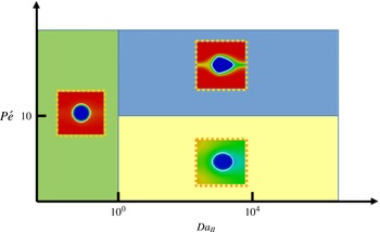
Figure 11. Regime diagram according to Péclet and Damköhler numbers.

Figure 12. Plot of the correction factor, $\unicode[STIX]{x1D6FC}$ , according to the Péclet and Damköhler numbers.

Figure 13. Plot of the evolution of the ratio between the correction factor, $\unicode[STIX]{x1D6FC}$ , computed according to (4.1), and the correction factor computed with (2.14).

These three different dissolution regimes differ from one another in the reactive surface accessible by the acid species, and we have seen that this is a strong function of the Damköhler and Péclet numbers. The macroscale dissolution rate, equation (2.13), involves a correction factor, $\unicode[STIX]{x1D6FC}$ , that represents the reduction of the reactive surface area accessible to acid contaminants due to the hydrodynamics. For all the simulation results, we computed the value of the correction factor for the first time steps for the fifth REV following the procedure described in § 2.2. The values of $\unicode[STIX]{x1D6FC}$ are plotted in figure 12. For $Da_{II}<1$ , all the surface available reacts homogeneously with the acid. In such case, the pillars keep their cylindrical shape and $\unicode[STIX]{x1D6FC}\rightarrow 1$ as theoretically demonstrated by Guo et al. (Reference Guo, Quintard and Laouafa2015) with the method of the volume averaging. For $1\leqslant Da_{II}<10^{4}$ , the correction factor decreases exponentially from 1 to 0 when $Da_{II}$ increases (see figure 12 a). Contrary to Guo et al. who suggested that the Péclet number has very low impact on the value of $\unicode[STIX]{x1D6FC}$ , our results show a strong dependency. For larger values of the Damköhler number ( $Da_{II}\geqslant 5\times 10^{4}$ ), the correction factor tends towards zero, in agreement with the theoretical results of Mauri (Reference Mauri1991) and Guo et al. (Reference Guo, Quintard and Laouafa2015) who showed that $\unicode[STIX]{x1D6FC}=O\left(Da_{II}^{-1}\right)$ when $Da_{II}\rightarrow \infty$ . This does not mean that the average dissolution rate described by (2.13) is zero, but that it becomes independent of the constant of reaction. This situation has been observed numerically for $Da_{II}\geqslant 5\times 10^{4}$ and $P\acute{e} >10$ . Nonlinear regression analysis shows that the correction factor, $\unicode[STIX]{x1D6FC}$ , can be described by the function

with $n=0.53$ and $m=0.88$ (less than 5 % of relative error). Note that $n\neq m$ , which emphasizes the strong nonlinear dissolution sub-regime that depends on the Péclet number when $1\leqslant Da_{II}<10^{4}$ . As the solid dissolves, the permeability, porosity and specific area evolve, and the Péclet and Damköhler numbers change accordingly. Equation (4.1) remains valid during the dissolution process as illustrated by the plot of the evolution of the ratio of $\unicode[STIX]{x1D6FC}$ computed with (4.1), where the Péclet and Damköhler numbers are evaluated in the current state of the medium and $\unicode[STIX]{x1D6FC}$ is computed with (2.14). Therefore, this formulation of the correction factor can be used directly to describe the dissolution rate of REV-based models.

We see from (2.13) that once the correction factor is determined, only the change of the effective surface area with time has to be estimated in order to close the system for Darcy-scale modelling. A number of different models based on geometrical constructions have been proposed to relate changes in porosity to changes in surface area (Lichtner Reference Lichtner1988; Emmanuel & Berkowitz Reference Emmanuel and Berkowitz2005; Noiriel et al. Reference Noiriel, Luquot, Madé, Raimbault, Gouze and van der Lee2009). In the case of a two-dimensional REV made up of a solid cylinder inside a square box ( $Da_{II}<1$ ), the relation between the surface area and porosity can be expressed as,

In (4.2), $A_{0}$ and $\unicode[STIX]{x1D719}_{0}$ correspond to the initial surface area and porosity, respectively. Surprisingly, this relation holds even when the solid pillar deviates from the cylindrical shape. Nevertheless, one has to be careful with the extrapolation of this relationship to more complex situations. For example, if the relationship of (4.2) is still valid for a 3-D porous medium made of cylinders, the exponent is $3/2$ instead of $1/2$ if the medium is made by a package of spherical grains. More complex models have also been proposed in the literature like the sugar lump model proposed by Noiriel et al. (Reference Noiriel, Luquot, Madé, Raimbault, Gouze and van der Lee2009) that assumes that the dissolution process dissociates the particles that composed the medium, which causes a significant increase in the surface area.

The permeability–porosity relation can be obtained by upscaling the pore-scale simulation results. For a given flow condition, i.e. $P\acute{e}$ and $Da_{II}$ , the evolution of the permeability in the fifth REV is obtained by volume averaging the velocity profile and pressure gradient and inverting Darcy’s law at every time step. Correlations to relate permeability and porosity in the form,

are sought, where $K_{0}$ and $\unicode[STIX]{x1D719}_{0}$ are the initial permeability and initial porosity. For all the simulations regardless of the dissolution regime, we obtain $p=3\pm 5\,\%$ and $q=2\pm 5\,\%$ by nonlinear regression.

4.2 Emergence of dissolution wormholes

We now consider the dissolution of a more complex pore space and we discuss the emergence of wormholes based on the flow conditions. The simulation set-up, i.e. geometry, fluid and rock properties, is based on the work of Song et al. (Reference Song, de Haas, Fadaei and Sinton2014) who conducted dissolution experiments in a real rock micro-model directly etched in a carbonate. It consists of multiple solid pillars, approximately $500~\unicode[STIX]{x03BC}\text{m}\times 500~\unicode[STIX]{x03BC}\text{m}$ , distributed uniformly in a $24~\text{mm}\times 7.2~\text{mm}$ two-dimensional domain. The pillars are aligned and separated from each other by $300~\unicode[STIX]{x03BC}\text{m}$ wide vertical and horizontal channels, as illustrated in figure 14. The porosity, permeability and specific area of the domain are estimated numerically to be $\unicode[STIX]{x1D719}_{0}\approx 0.76$ , $K_{0}=1.3\times 10^{-8}~\text{m}^{2}$ and $A_{0}=2310~\text{m}^{-1}$ , respectively. The computational domain is meshed using a $500\times 150$ Cartesian grid. The top and bottom boundaries are set as impermeable walls, i.e. no-slip boundary conditions. One per cent of acid is injected from the left-hand side of the domain at a constant velocity $v_{0}=10^{-3}~\text{m}~\text{s}^{-1}$ corresponding to $Re\approx 0.1$ . The right-hand side is an outflow condition. Simulation properties are set to $\unicode[STIX]{x1D707}_{f}=10^{-3}~\text{Pa}~\text{s}$ , $\unicode[STIX]{x1D70C}_{f}=1000~\text{kg}~\text{m}^{-3}$ , $\unicode[STIX]{x1D70C}_{s}=2165~\text{kg}~\text{m}^{-3}$ , $\unicode[STIX]{x1D6FD}=1$ and $k_{0}=10^{-15}~\text{m}^{2}$ .

Figure 14. Schematic of the two-dimensional porous medium. Blue corresponds to the void space ( $\unicode[STIX]{x1D700}_{f}=1$ ) and red to the solid ( $\unicode[STIX]{x1D700}_{f}=0.01$ ).

Figure 15. Prediction of the evolution of the pore space of a micro-model for different values of the constant of reaction and of the diffusion coefficient.

We performed multiple simulations with different reaction rates at the solid surface, ranging from $r=10^{-5}~\text{m}~\text{s}^{-1}$ to $r=10^{-1}~\text{m}~\text{s}^{-1}$ , and different diffusivity coefficients ranging from $D_{A}=10^{-10}~\text{m}^{2}~\text{s}^{-1}$ to $D_{A}=10^{-5}~\text{m}^{2}~\text{s}^{-1}$ . Similar to Song et al. (Reference Song, de Haas, Fadaei and Sinton2014) experiments, the acid is injected for $45~\text{min}$ . The time step was set to $\unicode[STIX]{x0394}t=10^{-3}~\text{s}$ . The simulations were performed on eight cores at the Stanford Center for Computational Earth and Environmental Sciences.

In line with other observations (Daccord, Lietard & Lenormand Reference Daccord, Lietard and Lenormand1993; Fredd & Fogler Reference Fredd and Fogler1998a ,Reference Fredd and Fogler b ; Golfier et al. Reference Golfier, Zarcone, Bazin, Lenormand, Lasseux and Quintard2002; Szymczak & Ladd Reference Szymczak and Ladd2009), the pore space structure after dissolution is significantly different according to the injection rate and the mineral reactivity. The simulation results exhibit five different dissolution patterns: (b) compact or facial dissolution, (c) conical wormhole, (d) one dominant wormhole, (e) ramified wormholes and (f) uniform dissolution. The $P\acute{e}$ – $Da_{I}$ diagram (figure 15 a) summarizes the different regimes obtained numerically according to the Péclet and the Damköhler numbers. The general features of the regime diagram agree well with the results of Golfier et al. (Reference Golfier, Zarcone, Bazin, Lenormand, Lasseux and Quintard2002) and Szymczak & Ladd (Reference Szymczak and Ladd2009). The transitions between the different regimes, however, differ from these studies. Several reasons can explain these discrepancies. First the characteristic lengths used to compute the Péclet and Damköhler numbers are not the same. In particular, the Péclet number (2.16) is evaluated from the square root of the permeability of the domain, $\sqrt{K}$ , and the second Damköhler number, $Da_{II}$ , from the specific surface area, $A_{e}^{-1}$ (2.17). Hence, the first Damköhler number, $Da_{I}$ , used to build the phase diagrams in Golfier et al. (Reference Golfier, Zarcone, Bazin, Lenormand, Lasseux and Quintard2002) and Szymczak & Ladd (Reference Szymczak and Ladd2009) is, in our study, weighted by $(\sqrt{K}A_{e})^{-1}$ (2.18). Second, the simulations of Golfier et al. (Reference Golfier, Zarcone, Bazin, Lenormand, Lasseux and Quintard2002) are based on a hybrid scale formulation that involves heuristic approximations for the permeability–porosity relationship and the dissolution rate in the block matrix while our simulation framework solves the directly physics at the pore scale.

For very small Péclet numbers ( $P\acute{e} \leqslant 10^{-2}$ ) and $Da_{I}>1$ , the concentration profile and the dissolution front are very stable as shown in figure 15(b). In this regime, usually qualified as compact, or facial dissolution, the flow is very slow, and the acid is transported to the mineral surface by diffusion only. For large values of the Damköhler number ( $Da_{I}>1$ ), the reaction is initiated as soon as the acid reaches the mineral surface. Because the consumption of acid at the pillars surface is fast, the progression of the acid in the domain is slowed down, which favours the dissolution of the pillars closer to the inlet. Moreover, because diffusion is the dominant mechanism for transport in the pore space, the concentration profile is homogeneous along the vertical cross-sections. When the acid reaches a row of solid grains, all the mineral is consumed before the concentration front propagates to the next row. Macroscopically, the average dissolution rate is linear (see figure 16 a) until all the grains are dissolved.

For $Da_{I}>1$ and larger injection rates, but still in a diffusion-dominated transport regime ( $1\geqslant P\acute{e} >10^{-2}$ ), the dissolution front is no longer uniform along the vertical cross-sections, and a faster region drags the dissolution front with it forming a conical pattern (figure 15 c). The acid penetrates into the matrix surrounding the conical wormhole mainly by diffusion. This leads to different characteristic times for the average dissolution rate, as illustrated in figure 16(a): in the early times of the dissolution process, the average rate of reaction is linear, and once the conical wormhole reaches the outlet of the domain, the slope is smoother because the diffusion is the dominant mechanism that brings acid at the surface of the grains surrounding the wormhole.

Figure 16. Plots of the average properties under different flow conditions. (a) Evolution of the mass of solid normalized by the initial mass, (b) permeability–porosity relationships, (c) specific area–porosity relationships.

For $Da_{I}>1$ and $10\geqslant P\acute{e} >1$ , we observe one dominant wormhole (figure 15 d). In this dissolution regime, the transport mechanism of acid in the void space is dominated by advection. Because the pore space heterogeneity generates important spatial variations in the velocity profile, the acid penetrates into the domain according to the faster region. Once a pillar disappears, it creates a pathway through which the acid flows preferentially. Moreover, diffusion is weak compared with advection; therefore, the transport of the acid from the wormhole to the matrix is limited to the grains surrounding the wormhole with the consequence of an aperture increase. Macroscopically, these dissolution mechanisms are described by two different slopes for the average dissolution rate (figure 16 a). Before the wormhole reaches the right-hand side of the domain, the slope is steep showing that the reaction of acid at the grain surface is fast. After breakthrough, the slope is less steep because smaller amounts of acid reach the solid grains in the matrix. This second part of the dissolution process will be a plateau if the matrix permeability is small compared with the wormhole aperture.

For $Da_{I}>1$ and $P\acute{e} >10$ the dissolution pattern is made up of ramified wormholes (figure 15 e). In this regime, advection is the strongest transport mechanism, and bifurcations of the local flow generate multiple dissolution pathways. The average dissolution exhibits two different slopes, but the transition between the two is less abrupt compared with the case of a single dominant wormhole.

Finally, for very small Damköhler number ( $Da_{I}\leqslant 1$ ) and regardless of the Péclet number, the dissolution of the grains is uniform (figure 15 f). In this regime, the characteristic time scale for the chemical reaction is longer than the transport time scale. Hence, the acid penetrates by convection and diffusion into the domain and contaminates almost the entire pore space. The acid at the solid surface is consumed at a smaller rate than the renewal rate leading to a homogeneous dissolution pattern. Compared with the other dissolution regimes, we see in figure 16(a) that for small Damköhler number the total rate of dissolution starts slow and then accelerates, while for larger $Da_{I}$ , it slows down during the process.

In addition to the evolution of the total mass of solid in the domain during the dissolution process, we also plot in figure 16 the permeability–porosity and the specific area–porosity relationships for the five different dissolution regimes. We observe nonlinear variations of the permeability–porosity according to the flow conditions. The variations are more important for regimes involving large wormholes, such as conical dissolution, or a single dominant wormhole. In these regimes, as soon as a wormhole reaches the domain outlet, the injected fluid flows preferentially along the new pathway created by the wormhole, which explains the large variations of the permeability. The flow resistance is then controlled by the aperture of the wormhole at the vicinity of the outlet. In the case of ramified wormholes, multiple preferential pathways percolate, and the variation although still important is smoother. For the compact and uniform dissolution regimes, there are no large channels to favour the flow from the inlet to the outlet, and the flow is limited by the porous medium pore throats. Figure 16(c) shows that the specific area–porosity relationship does not vary noticeably with the dissolution regimes.