


1. Introduction
Flows in rapidly rotating containers are of fundamental interest in a range of geophysical and engineering applications (Kerswell Reference Kerswell2002; Le Bars, Cebron & Le Gal Reference Le Bars, Cebron and Le Gal2015). Here, we deal with incompressible flows in cylindrical containers. If, as well as rotating around its symmetry axis, the cylinder is precessionally forced, i.e. the solid-body rotation vector itself is rotating about another axis tilted at an angle  $\alpha$ with respect to the first and at a different frequency, an overturning flow is driven within the cylinder. This forced overturning flow has azimuthal wavenumber
  $m={\pm }1$; it is due to this component of the velocity that the flow can cross the axis of the cylinder (Batchelor & Gill Reference Batchelor and Gill1962). The amplitude of the precessional forcing that drives the overturning flow is proportional to the product of the ratio of precession and rotation frequencies (the Poincaré number
  $Po=\varOmega _p/\varOmega _c$, where
  $\varOmega_p$ and
  $\varOmega_c$ are respectively precessional and cylinder angular speeds, see table 1) and the sine of the tilt angle,
  $|Po\sin \alpha |$. The precessionally forced flow can become relatively large even if
  $|Po\sin \alpha |\ll 1$, provided the dimensionless forcing frequency
  $\omega _f=1/(1+Po\cos \alpha )$ is tuned to resonate with an intrinsic inertial mode. These modes, known as Kelvin modes, are found via separation of variables in the linear inviscid limits; they have Bessel function structure in the radial direction, are harmonic in the axial and azimuthal directions, and are harmonic in time with frequencies greater than zero and less than twice the background solid-body rotation frequency (Kelvin Reference Kelvin1880; Fultz Reference Fultz1959; Greenspan Reference Greenspan1968). The resulting large-amplitude forced response may then excite other inertial modes via triadic resonance. These topics have been addressed in many past studies (Manasseh Reference Manasseh1992; Kobine Reference Kobine1996; Kerswell Reference Kerswell1999; Lagrange et al. Reference Lagrange, Meunier, Nadal and Eloy2011; Albrecht et al. Reference Albrecht, Blackburn, Lopez, Manasseh and Meunier2015; Marques & Lopez Reference Marques and Lopez2015; Herault et al. Reference Herault, Gundrum, Giesecke and Stefani2015; Kong et al. Reference Kong, Cui, Liao and Zhang2015; Lopez & Marques Reference Lopez and Marques2016; Albrecht et al. Reference Albrecht, Blackburn, Lopez, Manasseh and Meunier2018; Lopez & Marques Reference Lopez and Marques2018; Giesecke et al. Reference Giesecke, Vogt, Gundrum and Stefani2018; Herault et al. Reference Herault, Giesecke, Gundrum and Stefani2019).
Table 1. Definitions of angular velocity terms; also see figure 1.

Our primary focus in the present work rests not so much on these resonant effects, but rather on the space–time mean flow which occurs in the cylinder, i.e. the steady streaming (Riley Reference Riley2001) forced by precession, and details of the source terms that drive it. Before proceeding, it is worthwhile to define what we mean by the steady streaming flow in a situation where, as here, the flow could be both temporally and spatially oscillatory. We define steady streaming as the temporal and azimuthal average of the precessionally forced flow in the rotating cylinder. It is assumed that the forced flows have reached statistically steady states such that the concept of a long-time temporal average is meaningful. It makes no difference to the outcome in which order these two averages are taken. We note that this definition of steady streaming differs from the definition of (unsteady) streaming used by Marques & Lopez (Reference Marques and Lopez2015), who defined streaming to be the azimuthally averaged flow, which could vary in time, i.e. the axisymmetric ( $m=0$) Fourier component of the precessionally forced flow. If the flow is a steadily rotating wave in some frame of reference, this azimuthal average is also the space–time average. Henceforth we will just refer to the streaming flow (or simply, streaming) on the understanding that we refer to the space–time average. The streaming is constant in both time and azimuthal coordinate, but may vary radially and axially within the cylinder. Its magnitude squared is a measure of the rate at which energy is taken from the viscous and pressure work done at the boundary of the precessing cylinder. The streaming flow is axisymmetric, but it is not purely azimuthal (so-called zonal); it may possess significant meridional (i.e. radial and axial) velocity components. For the cases we have examined, the azimuthal velocity component is strongest (and significantly non-uniform in the axial direction). The azimuthal average of the streaming typically amounts to an azimuthal (zonal) flow that is retrograde with respect to the mean rotation of the cylinder. Streaming is of interest not only in and of itself, but also because of the role it may play in the saturation of the overturning flow through detuning effects (Meunier et al. Reference Meunier, Eloy, Lagrange and Nadal2008). That detuning may in turn dampen triadic-resonance instabilities, leading to finite-amplitude saturation or intermittency of unstable modes, rather than a fully developed transition to turbulence (Lagrange et al. Reference Lagrange, Meunier, Nadal and Eloy2011; Herault et al. Reference Herault, Giesecke, Gundrum and Stefani2019). Finally, streaming is a very efficient source of dynamo action (Giesecke et al. Reference Giesecke, Vogt, Gundrum and Stefani2018, Reference Giesecke, Vogt, Gundrum and Stefani2019).
It is natural to consider the source terms for the streaming to derive from Reynolds stresses, and that has been the assumption in many previous discussions since the considered flows from which the streaming derives were wavy in some sense. A key goal of this work is to demonstrate that for the precessing flow considered an additional source derives from a direct Coriolis-type interaction with the overturning flow (rather than self-interactions inherent in Reynolds stresses), and that streaming due to this source may be the dominant component. By direct Coriolis-type interaction, we mean the non-zero time- and azimuthally averaged source term arising from the Coriolis term. This contains the product of a time-varying  $m={\pm }1$ flow, such as that driven at leading order by precession, and a time-varying component of the rotation rate, which in precession also has
  $m={\pm }1$. Just as with the Reynolds stresses, time averaging the product of these two fluctuating quantities leads to a non-zero source term capable of driving a streaming flow. Naturally, any Navier–Stokes, or even Euler, equations simulation would automatically capture this term, so that streaming flows have featured in very many simulations of precessing flows, (e.g. Kong, Liao & Zhang Reference Kong, Liao and Zhang2014; Jiang et al. Reference Jiang, Kong, Zhu and Zhang2015; Kong et al. Reference Kong, Cui, Liao and Zhang2015; Marques & Lopez Reference Marques and Lopez2015; Lopez & Marques Reference Lopez and Marques2016; Wu, Welfert & Lopez Reference Wu, Welfert and Lopez2020). However, the contribution of this Coriolis-type term to the streaming flow has been unrecognised. In studies that have a more analytical rather than simulation basis (Busse Reference Busse1968; Tilgner Reference Tilgner2007), interactions in viscous boundary layers were investigated without examining the direct Coriolis-type interaction. In other studies (Greenspan Reference Greenspan1969; Kerswell Reference Kerswell1999), the flow was presumed to have a basis of inertial modes, and their interactions were investigated as a source of the streaming, again ignoring the direct Coriolis-type term. Importantly, the direct Coriolis-type interaction requires only the existence of a time-varying flow and a time-varying rotation rate with the same azimuthal structure. This will occur generically in precessing fluids, irrespective of whether or not inertial oscillations are present.
In § 2 we develop equations for the viscous streaming flow in precessing vessels, showing in detail how the two types of source terms arise. In § 3 we analyse three example flows which fall within the weak streaming regime, i.e. where the overturning flow is weak enough that the equations for the streaming flow are very close to linear and so we can examine separately the streaming that results from the Coriolis and Reynolds-stress mechanisms. In all cases, the azimuthal component of streaming is dominant over the meridional components, and has significant axial structure. The first of these examples (§ 3.1) is a case in which the forcing frequency is larger than twice the background solid-body rotation frequency, no inertial modes are resonantly excited and so the forced overturning flow does not become large, while the second case (§ 3.2) is resonantly tuned resulting in a forced overturning flow that is relatively much larger than in the first case, even though the imposed forcing amplitude,  $|Po\sin \alpha |$, is smaller. In the third example case (§ 3.3), the forced overturning flow, which is also tuned to resonantly excite the
  $m={\pm }1$ intrinsic Kelvin mode, becomes large enough to support a saturated triadic-resonance instability with two free Kelvin modes with azimuthal wavenumbers
  $m={\pm }5$ and
  $m={\pm }6$ whose frequencies also meet the conditions for triadic resonance. While the structure of the resulting streaming is broadly similar to that for the lower-amplitude case of § 3.2, the analysis of this case is (in § A.3) expanded in order to examine separately the contributions of Reynolds stresses associated with the two free Kelvin modes involved in the triadic resonance. Section 4 provides a parametric examination of how the magnitude of streaming varies with the magnitude of the overturning flow, Reynolds number, tilt angle, Poincaré number and cylinder aspect ratio, predominantly for cases where the overturning flow is resonant but not subject to instability. This examination facilitates a rational modification to a quasi-analytical model equation for the amplitude of the axisymmetric flow (Meunier et al. Reference Meunier, Eloy, Lagrange and Nadal2008) in order to accommodate Coriolis forcing terms. Those terms were originally neglected in the original model because they arise at a higher order than the nonlinear terms in the asymptotic theory. That equation, in turn, forms a key element of weakly nonlinear amplitude equations used for the prediction of triadic resonance instability in precessing cylinders; see § 6.3 of Lagrange et al. (Reference Lagrange, Meunier, Nadal and Eloy2011).
2. Problem description and methodology
As shown schematically in figure 1(a), we consider an incompressible viscous flow in a cylinder of height  $H$ and radius
  $R$ that is mounted on a turntable via a gimbal which allows the cylinder axis to be tilted through angle
  $\alpha$. The cylinder rotates with an angular velocity
  $\boldsymbol {\varOmega }_c$ that precesses at angular velocity
  $\boldsymbol {\varOmega }_p$ with respect to the turntable axis. In a Cartesian coordinate system fixed to the gimbal, the unit vector aligned along the cylinder axis is denoted
  $\boldsymbol {e}_z$, the unit basis vector aligned with the gimbal tilt axis is denoted
  $\boldsymbol {e}_y= \boldsymbol {\varOmega }_c\times \boldsymbol {\varOmega }_p/ |\boldsymbol {\varOmega }_c\times \boldsymbol {\varOmega }_p|$, and the remaining orthogonal unit vector is
  $\boldsymbol {e}_x$; see figure 1(b). Without loss of generality,
  $\varOmega _c=\boldsymbol {\varOmega }_c\boldsymbol {\cdot }\boldsymbol {e}_z$ is taken to be positive and
  $\varOmega _p=|\boldsymbol {\varOmega }_p|\operatorname {sgn}(\boldsymbol {\varOmega }_p\boldsymbol {\cdot }\boldsymbol {e}_z)$. Both
  $\varOmega _c$ and
  $\varOmega _p$ are constant since the cylinder and turntable each rotate steadily. Precession is prograde (retrograde) with respect to
  $\boldsymbol {\varOmega }_c$ if
  $\varOmega _p>0$ (
 $<0$). The Poincaré number,
 \begin{equation} Po=\frac{\varOmega_p}{\varOmega_c}, \end{equation}
is thus positive for prograde and negative for retrograde precession. The non-dimensional frequency of precessional forcing is
 \begin{equation} \omega_f=\frac{\varOmega_c}{\varOmega_c+\varOmega_p\cos\alpha} = \frac{1}{1+Po\cos\alpha}, \end{equation}
and the magnitude of precessional forcing is proportional to  $|Po\sin \alpha |$.

Figure 1. (a) Schematic of the precessing flow configuration, (b) top view of cylinder with gimbal axis system and (c) cylindrical coordinate system  $(r,\varphi ,z)$ and orientation of the meridional semi-plane shown in subsequent figures.
The total rotation-rate vector,  $\boldsymbol {\varOmega }_c+\boldsymbol {\varOmega }_p$, can be decomposed into an axial component
  $\boldsymbol {\varOmega }_{\parallel }$ aligned with
  $\boldsymbol {e}_z$ and an equatorial-plane component
  $\boldsymbol {\varOmega }_{\perp }$ aligned with
  $\boldsymbol {e}_x$. Their magnitudes are
  $|\boldsymbol {\varOmega }_{\parallel }|=|\varOmega _c+\varOmega _p\cos \alpha |$ and
  $|\boldsymbol {\varOmega }_{\perp }|=|\varOmega _p\sin \alpha |$. Ultimately, it is
  $\boldsymbol {\varOmega }_{\perp }$ that drives the overturning flow inside the cylinder. A simple but important point in what follows is that when expressed in cylindrical coordinates
  $(r,\varphi ,z)$ (see figure 1c),
  $\boldsymbol {\varOmega }_{\perp }$ has only radial and azimuthal components, which are
  $2{\rm \pi}$-periodic in azimuth
  $\varphi$, whereas
  $\boldsymbol {\varOmega }_{\parallel }$ has only a constant axial component. For reference, the nomenclature for various angular velocity terms adopted herein is summarised in table 1.
2.1. Equations for and sources of streaming flow in rotating cylindrical coordinates
The flow is governed by the incompressible Navier–Stokes equations in a rotating frame of reference (typically, either the cylinder or the gimbal frame), non-dimensionalised with length scale  $R$ and time scale
  $1/|\boldsymbol {\varOmega }_{\parallel }|$; these are
 \begin{equation} \frac{\partial \boldsymbol{u}}{\partial t} +\boldsymbol{\nabla}\boldsymbol{\cdot}(\boldsymbol{uu})+ \left(2\boldsymbol{{\varOmega}}\times\boldsymbol{{u}}\right) + \left(\frac{\mathrm{d} \boldsymbol{\varOmega}}{\mathrm{d} t} \times \boldsymbol{r}\right) + \boldsymbol{\nabla}{p} - \frac{1}{Re}\nabla^2\boldsymbol{{u}} = 0,\quad \boldsymbol{\nabla}\boldsymbol{\cdot} \boldsymbol{u}=0, \end{equation}
where the Reynolds number (or inverse Ekman number) is
 \begin{equation} Re=\left|\boldsymbol{\varOmega}_{\parallel}\right|\frac{R^2}{\nu} =\left|\varOmega_c+\varOmega_p\cos\alpha\right|\frac{R^2}{\nu} =\left|\varOmega_c(1+Po\cos\alpha)\right|\frac{R^2}{\nu} =\left|\frac{\varOmega_c}{\omega_f}\right|\frac{R^2}{\nu}. \end{equation}
The flow is governed by four independent dimensionless groups, which we take as  $Re$,
$Re$,  $\omega _f$,
  $\alpha$ and
  $H/R$. Unlike what holds for many other forced rotating systems, it is not straightforward to independently vary either the forcing amplitude or the forcing frequency while maintaining all other governing parameters constant.
The position vector  $\boldsymbol {r}$ gives the location of any point with respect to the origin of the chosen reference frame,
  $\boldsymbol {u}$ is the associated fluid velocity and
  $\boldsymbol {\varOmega }$ is the associated rotation vector. The terms
  $2\boldsymbol {\varOmega }\times \boldsymbol {u}$ and
  $(\mathrm {d} \boldsymbol {\varOmega } / \mathrm {d} t) \times \boldsymbol {r}$ are the Coriolis and Euler force terms. Potential terms associated with centripetal acceleration are, along with the fluid density, absorbed into the reduced pressure
  $p$, and the velocity boundary conditions are no slip on the walls of the cylinder.
The rotating frame of reference may be taken as attached to either the gimbal or the cylinder. In the gimbal frame, the rotation vector is  $\boldsymbol {\varOmega }=(\varOmega _p\cos \alpha )\boldsymbol {e}_z+|\boldsymbol {\varOmega }_{\perp }|\boldsymbol {e}_x$; it is fixed and the cylinder walls rotate about the axis at rate
  $\varOmega _c$. In the cylinder frame of reference, the rotation vector is
  $\boldsymbol {\varOmega }=\boldsymbol {\varOmega }_c+\boldsymbol {\varOmega }_p =\boldsymbol {\varOmega }_{\parallel }+\boldsymbol {\varOmega }_{\perp }$, which is identical to the inertial-frame rotation vector, and only the axial component of rotation
  $\boldsymbol {\varOmega }_{\parallel }=(\varOmega _c+\varOmega _p\cos \alpha )\boldsymbol {e}_z$ is fixed, while the equatorial component, of constant magnitude
  $|\boldsymbol {\varOmega }_{\perp }|$, rotates steadily about the cylinder axis at rate
  $-\varOmega _c$. The magnitude of the equatorial component,
  $|\boldsymbol {\varOmega }_{\perp }|$, is the same in either of these two frames. In the gimbal frame of reference, there is no Euler force since
  $\mathrm {d}\boldsymbol {\varOmega }/\mathrm {d} t=0$ and the cylinder walls rotate with respect to the observer, whereas in the cylinder frame there is an Euler force associated with the continuous change in direction of
  $\boldsymbol {\varOmega }_{\perp }$ and the cylinder walls appear stationary. For simplicity, we will henceforth principally restrict attention to the cylinder frame of reference, but include in appendix A further considerations of streaming in the gimbal frame of reference.
Our focus is on the azimuthally and temporally averaged flow, i.e. the steady and axisymmetric streaming flow in azimuthal Fourier mode  $m=0$. Fourier transforming the momentum equation of (2.3) in azimuth and taking
  $m=0$ gives
 \begin{equation} \frac{\partial\hat{\boldsymbol{u}}_0}{\partial t} + \left[\boldsymbol{\nabla} \boldsymbol{\cdot}(\boldsymbol{uu})\right]^{\wedge}_0 + 2\left[\boldsymbol{\varOmega}\times\boldsymbol{u}\right]^{\wedge}_0 + \left[\frac{\mathrm{d} \boldsymbol{\varOmega}}{\mathrm{d} t}\times\boldsymbol{r}\right]^{\wedge}_0 + \boldsymbol{\nabla}\hat{p}_0 - \frac{1}{Re}\nabla^2\hat{\boldsymbol{u}}_0 = 0, \end{equation}
where numeric subscripts denote the azimuthal wavenumber  $m$ of a Fourier-transformed variable, indicated by
  $^{\wedge }$. The axisymmetric (
 $m=0$) component of the Euler force term,
  $[({\mathrm {d} \boldsymbol {\varOmega }}/{\mathrm {d} t})\times \boldsymbol {r}]^{\wedge }_0=0$ since in the cylinder frame the temporal variation only makes contributions in
  $m={\pm }1$, and so the Euler force will only appear indirectly in the equation for
  $m=0$ (via forcing terms involving
  $\hat {\boldsymbol {u}}_{{\pm }1}$). Applying the convolution theorem to (2.5) gives
 \begin{equation} \frac{\partial\hat{\boldsymbol{u}}_0}{\partial t} + \sum_{j+k=0}\boldsymbol{\nabla}\boldsymbol{\cdot}(\hat{\boldsymbol{u}}_j \hat{\boldsymbol{u}}_k) + 2\!\sum_{j+k=0}\hat{\boldsymbol{\varOmega}}_j\times\hat{\boldsymbol{u}}_k + \boldsymbol{\nabla}\hat{p}_0 - \frac{1}{Re}\nabla^2\hat{\boldsymbol{u}}_0=0, \quad j,k\in\mathbb{I}. \end{equation}
Since all the terms are real in physical space, in Fourier space all the complex vector fields for non-zero azimuthal wavenumbers have conjugate symmetry, e.g.  $\hat {\boldsymbol {u}}_{+1}=\hat {\boldsymbol {u}}_{-1}^{\ast }$, where
  $^{\ast }$ denotes complex conjugation. For
  $m=0$, all fields are real. As should be apparent from the discussion immediately preceding § 2.1, the only non-zero
  $\hat {\boldsymbol {\varOmega }}_j$ occur in wavenumbers
  $m=0,{\pm }1$.
Rearranging (2.6) to separate between  $m=0$ and
  $m\ne 0$ contributions,
 \begin{align} \frac{\partial\hat{\boldsymbol{u}}_0}{\partial t} + \boldsymbol{\nabla}\boldsymbol{\cdot}(\hat{\boldsymbol{u}}_0\hat{\boldsymbol{u}}_0) + 2\hat{\boldsymbol{\varOmega}}_0\times\hat{\boldsymbol{u}}_0 + \boldsymbol{\nabla}\hat{p}_0- \frac{1}{Re}\nabla^2\hat{\boldsymbol{u}}_0 &= - 2 (\hat{\boldsymbol{\varOmega}}_{-1}\times\hat{\boldsymbol{u}}_1+ \hat{\boldsymbol{\varOmega}}_{1}\times\hat{\boldsymbol{u}}_{-1})\nonumber\\ &\quad- \sum_{m\!{\ne}0}\boldsymbol{\nabla}\boldsymbol{\cdot}(\hat{\boldsymbol{u}}_{m}\hat{\boldsymbol{u}}_{-m}). \end{align}
In the cylinder frame  $\hat {\boldsymbol {\varOmega }}_0\equiv \boldsymbol {\varOmega }_{\parallel }= (\varOmega _c+\varOmega _p\cos \alpha )\boldsymbol {e}_z$ is steady and
  $\hat {\boldsymbol {\varOmega }}_{{\pm }1}$ are temporally harmonic.
  $\hat {\boldsymbol {\varOmega }}_0$ is purely axial and real, while
  $\hat {\boldsymbol {\varOmega }}_{{\pm }1}$ (the Fourier projection of
  $\boldsymbol {\varOmega }_{\perp }$) are purely equatorial and complex.
On the right-hand side of (2.7), there are, in addition to the conventional Reynolds-stress-type driving terms for the azimuthally averaged flow (such as would appear for an unsteady flow in a non-rotating frame), new terms involving cross-products of the equatorial-plane component of reference-frame rotation and flow velocity in azimuthal wavenumbers  $m={\pm }1$. These terms are particular to flows in axisymmetric precessing vessels. In physical space, these terms can be regarded as resulting from the cross-product of the equatorial component of the total rotation vector with the three-dimensional velocity field. Only terms involving Fourier modes
  $m={\pm }1$ are involved in
  $\boldsymbol {\mathcal {C}}'$ because
  $\boldsymbol {\varOmega }_{\perp }$ projects exactly onto these wavenumbers, and because (2.7) is the equation for
  $m=0$. One can also consider
  $\boldsymbol {\mathcal {C}}'$ in physical space as resulting from the cross-product of
  $\boldsymbol {\varOmega }_{\perp }$ with the restriction of
  $\boldsymbol {u}$ to components with
  $2{\rm \pi}$-cyclic variation in azimuthal coordinate
  $\varphi$. Since they do not appear to have an accepted name, we will adopt the phrase ‘equatorial-Coriolis forcing’ for these cross-product terms. Also of note is the fact that owing to symmetry and parity conditions at the axis, only flows with
  $\hat {\boldsymbol {u}}_{{\pm }1}\ne \boldsymbol {0}$ can cross the axis (Batchelor & Gill Reference Batchelor and Gill1962; Marques & Lopez Reference Marques and Lopez2001; Blackburn & Sherwin Reference Blackburn and Sherwin2004). As a result, they involve large-scale overturning flows which extend throughout the whole cylinder. Indeed, for all the cases considered, the overturning flow is dominated by contributions in
  $m={\pm }1$.
Equation (2.7) describes the evolution of the azimuthally averaged flow. To obtain the streaming flow further requires temporal averaging. Introducing the Reynolds decompositions
 \begin{align} \boldsymbol{u}(\boldsymbol{r},t)=\overline{\boldsymbol{u}}(\boldsymbol{r})+\boldsymbol{u}'(\boldsymbol{r},t),\quad p(\boldsymbol{r},t)=\overline{p}(\boldsymbol{r})+p'(\boldsymbol{r},t) \quad \text{and}\quad \boldsymbol{\varOmega}(\boldsymbol{r},t) =\overline{\boldsymbol{\varOmega}}(\boldsymbol{r})+\boldsymbol{\varOmega}'(\boldsymbol{r},t) \end{align}
into (2.7), and time averaging, leads to the equation for the streaming flow  $\overline {\hat {\boldsymbol {u}}}_0$,
 \begin{equation} \boldsymbol{\nabla}\boldsymbol{\cdot}\left(\overline{\hat{\boldsymbol{u}}}_0\overline{\hat{\boldsymbol{u}}}_0\right) + 2\overline{\hat{\boldsymbol{\varOmega}}}_0\times\overline{\hat{\boldsymbol{u}}}_0 + \boldsymbol{\nabla}\overline{\hat{p}}_0 - \frac{1}{Re}\nabla^2\overline{\hat{\boldsymbol{u}}}_0 = - \boldsymbol{\nabla}\boldsymbol{\cdot}\left(\overline{\hat{\boldsymbol{u}}'_0\hat{\boldsymbol{u}}'_0}\right) + \boldsymbol{\mathcal{C}}' + \boldsymbol{\mathcal{R}}', \end{equation}
where, in the cylinder frame
 \begin{equation} \boldsymbol{\mathcal{C}}' = - 2\left(\overline{\hat{\boldsymbol{\varOmega}}'_{-1}\times\hat{\boldsymbol{u}}'_1} + \overline{\hat{\boldsymbol{\varOmega}}'_{1}\times\hat{\boldsymbol{u}}'_{-1}}\right) \quad \text{and}\quad \boldsymbol{\mathcal{R}}' = - \sum_{m\!{\ne}0} \boldsymbol{\nabla}\boldsymbol{\cdot}\left(\overline{\hat{\boldsymbol{u}}'_m\hat{\boldsymbol{u}}'_{-m}}\right) \end{equation}
are respectively equatorial-Coriolis and Reynolds-stress source terms generating the streaming flow (corresponding relations for the gimbal frame of reference are provided in appendix A). In (2.9), all terms but one are steady, two-dimensional and three-component real vector fields. The exception is  $\boldsymbol {\nabla }\overline {\hat {p}}_0$, which is a steady two-dimensional, two-component real vector field since
  $p$ is a scalar; this term has no azimuthal component. In all cases examined here,
  $\boldsymbol {u}_0$ is steady and so
  $\overline {\hat {\boldsymbol {u}}'_0\hat {\boldsymbol {u}}'_0}=0$.
2.2. Solution methodology
A two-pronged approach is used to obtain the results we present below. First, we use three-dimensional direct numerical simulation (DNS, detailed in § 2.3) to obtain the full solution to (2.3), integrating sufficiently long in time that the first- and second-order statistics converge, thus providing the source terms for (2.10a,b). We then use these to drive a two-dimensional (axisymmetric) restriction of (2.3) – i.e. the unsteady equivalent of (2.9), with terms  $\boldsymbol {\mathcal {C}}'$ and
  $\boldsymbol {\mathcal {R}}'$ obtained by post-processing full DNS results – to steady state and confirm that this solution is at better than single-precision accuracy identical to the azimuthal and temporal average of the full DNS. Our approach thus enables us to firmly establish the sources of the streaming flow.
For the cases examined, the total streaming is also, to within visual plotting accuracy, the superposition of the flows driven by the terms in (2.10a,b) taken individually, which implies that the nonlinear term  $\boldsymbol {\nabla }\boldsymbol {\cdot }\left (\overline {\hat {\boldsymbol {u}}}_0\overline {\hat {\boldsymbol {u}}}_0\right )$ is negligibly small, and all cases thus fall in the weak streaming regime, for which (2.9) is nearly linear. As already remarked,
  $\overline {\hat {\boldsymbol {u}}'_0\hat {\boldsymbol {u}}'_0}=0$ for the flows examined here. Thus, to a good approximation (2.9) can be simplified to
 \begin{equation} 2\left(\overline{\hat{\boldsymbol{\varOmega}}}_0\times\overline{\hat{\boldsymbol{u}}}_0\right) + \boldsymbol{\nabla}\overline{\hat{p}}_0 - \frac{1}{Re}\nabla^2\overline{\hat{\boldsymbol{u}}}_0 = \boldsymbol{\mathcal{C}}' + \boldsymbol{\mathcal{R}}', \end{equation}
whose radial, azimuthal and axial components are
 \begin{gather} \frac{\partial \overline{\hat{p}}_0}{\partial r} -\frac{1}{Re}\left[\frac{\partial^2}{\partial z^2} +\frac{\partial^2}{\partial r^2} + \frac{1}{r}\frac{\partial}{\partial r} -\frac{1}{r^2}\right]\overline{\hat{u}}_0= \mathcal{C}'_r+\mathcal{R}'_r + 2\overline{\hat{\varOmega}}_0\overline{\hat{v}}_0, \end{gather}
 \begin{gather}-\frac{1}{Re}\left[\frac{\partial^2}{\partial z^2} +\frac{\partial^2}{\partial r^2} + \frac{1}{r}\frac{\partial}{\partial r} -\frac{1}{r^2}\right]\overline{\hat{v}}_0= \mathcal{C}'_{\varphi}+\mathcal{R}'_{\varphi} - 2\overline{\hat{\varOmega}}_0\overline{\hat{u}}_0, \end{gather}
 \begin{gather}\frac{\partial \overline{\hat{p}}_0}{\partial z} -\frac{1}{Re}\left[\frac{\partial^2}{\partial z^2} +\frac{\partial^2}{\partial r^2} +\frac{1}{r}\frac{\partial}{\partial r}\right]\overline{\hat{w}}_0= \mathcal{C}'_z+\mathcal{R}'_z, \end{gather}
where in the forcing terms we observe the standard rotating-frame coupling between radial and azimuthal components (i.e. a positive azimuthal velocity drives an increase in radial velocity, while a positive radial velocity drives a decrease in azimuthal velocity), and there is no pressure gradient term in the equation for the azimuthal streaming, (2.12b).
2.3. Numerical methods
The numerical methods employed, which use spectral elements to discretise the meridional semi-plane and Fourier expansions in azimuth, have been previously described in Blackburn & Sherwin (Reference Blackburn and Sherwin2004), Blackburn et al. (Reference Blackburn, Lee, Albrecht and Singh2019) and Albrecht et al. (Reference Albrecht, Blackburn, Lopez, Manasseh and Meunier2015, Reference Albrecht, Blackburn, Meunier, Manasseh and Lopez2016, Reference Albrecht, Blackburn, Lopez, Manasseh and Meunier2018); the latter references also provide comparisons to experimental results for precessing cylinder flows with triadic resonance instabilities. For the example cases presented in § 3, and as in Lagrange et al. (Reference Lagrange, Eloy, Nadal and Meunier2008) and § 4.1 of Albrecht et al. (Reference Albrecht, Blackburn, Lopez, Manasseh and Meunier2015), we consider  $H/R=1.62$. A representative spectral element mesh employed for the simulations in § 3 is shown in figure 2: each element has shape functions with tensor products of sixth-order Lagrange interpolants through the Gauss–Lobatto–Legendre points. The total number of mesh degrees of freedom for two-dimensional solutions is 27 985, while for three-dimensional solutions, which have 128 azimuthal planes (64 Fourier modes) of data, the total number of mesh degrees of freedom is approximately
  $3.5\times 10^6$. For the cases examined in § 3, we fix
  $Re=6500$ (comparable to that used in the experiments of Lagrange et al. (Reference Lagrange, Eloy, Nadal and Meunier2008)), and vary
  $\omega _f$ and
  $\alpha$. In § 4, we consider simulations at other aspect ratios and Reynolds numbers, and with comparable resolutions.

Figure 2. Spectral element mesh for the meridional semi-plane, with 628 elements. For three-dimensional DNS, 128 planes of data are used in azimuth.
3. Results
3.1. Case 1:  $\omega _f=2.5$, $\alpha =0.4^{\circ }$, $Re=6500$ and $H/R=1.62$


We commence by considering a case at forcing frequency  $\omega _f=2.5$, which is larger than twice the background solid-body rotation frequency, so that inertial wave-type phenomena such as Kelvin-related eigenmodes or wave beams are not expected to be present. The tilt angle
  $\alpha =0.4^{\circ }$ is small and the three-dimensional flow is a rotating wave in the cylinder frame (steady in the gimbal frame). The Poincaré number is
  $Po=-0.6$, so the precessional forcing, proportional to
  $|Po\sin \alpha |=4.19\times 10^{-3}$, is small. In the gimbal frame, the flow can be conceptualised as a combination of solid-body rotation (with azimuthal wavenumber
  $m=0$) and a steady overturning flow, dominated by contributions in azimuthal wavenumber
  $m={\pm }1$, driven by precession.
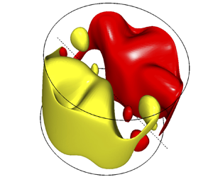
A perspective view of the flow is represented in figure 3 by two isosurfaces of axial velocity of equal magnitude and opposite sign. (The axial velocity component is a useful diagnostic since it is the same in cylinder and gimbal frames.) It should be apparent that this flow is dominated by overturning with contributions in azimuthal wavenumbers  $m={\pm }1$. The axial velocities are small since the precessional forcing is small, inertial waves are not excited, and the Reynolds number is only moderately large. Apart from thin boundary layers near the walls, the shape and magnitude of the isosurfaces suggest a slow and structurally simple overturning flow that fills the whole container and whose streamlines have the form of closed loops that lie orthogonal to
  $\boldsymbol {\varOmega }_{\perp }$, so that equatorial-Coriolis accelerations
  $\boldsymbol {\varOmega }_{\perp }\times \boldsymbol {u}$ are close to zero in the gimbal frame of reference; this is the equilibrium azimuthal orientation of a steady non-resonant overturning flow.

Figure 3. Isosurfaces of axial velocity at levels  $w={\pm }0.01$ for case 1:
  $\omega _f=2.5$,
  $\alpha =0.4^{\circ }$, showing the nature of the overturning flow when resonant effects are absent. The dashed line represents the gimbal tilt axis (cf. figure 1b). Flow is steady in the gimbal frame of reference.
In order to gauge the overall strength of the flow driven by precessional forcing compared to solid-body rotation of the basic flow in an inertial frame of reference ( $\boldsymbol {u}_{sb}=\boldsymbol {\varOmega }_c\times \boldsymbol {r}$) one may compute a Rossby number
  $Ro_{3D}=[E(\boldsymbol {u})/E(\boldsymbol {u}_{sb})]^{1/2}$ where
  $E$ is flow kinetic energy integrated over the volume of the cylinder. For the present case,
  $Ro_{3D}=1.70\times 10^{-3}$.
We next consider the streaming flow and source terms for this case. These are shown in figure 4, whose upper panels, (a–i), show source terms, while lower panels, (j–u), show the resulting streaming flow. Recalling § 2.2, we re-iterate that our methodology is first to use three-dimensional DNS in order to collect statistics for source terms ( $\boldsymbol {\mathcal {C}}'$,
  $\boldsymbol {\mathcal {R}}'$, etc.), while we can compute the streaming flow
  $\overline {\hat {\boldsymbol {u}}}_0$ in a variety of ways: (i) as the temporal and azimuthal average of the three-dimensional DNS; (ii) using two-dimensional DNS driven by the sum of source terms e.g.
  $\boldsymbol {\mathcal {C}}'+\boldsymbol {\mathcal {R}}'$; (iii) as the sum of two-dimensional DNS computations driven independently by the equatorial-Coriolis source terms (
 $\boldsymbol {\mathcal {C}}'$) and the Reynolds-stress source terms (
 $\boldsymbol {\mathcal {R}}'$). This means that the results shown in figure 4(j–m) in could equally well be obtained via methods (i) or (ii), whereas the results in panels (n–q) and (r–u) were obtained using two-dimensional DNS restrictions driven respectively by
  $\boldsymbol {\mathcal {C}}'$ and
  $\boldsymbol {\mathcal {R}}'$. The fact that the resulting flows are the same for (i) and (ii) serves as a cross-check on the methodology, while the fact that these results agree to within plotting accuracy with those obtained using method (iii) shows that the streaming is weak, i.e.
  $\boldsymbol {\nabla }\boldsymbol {\cdot }(\overline {\hat {\boldsymbol {u}}}_0\overline {\hat {\boldsymbol {u}}}_0)\approx 0$, which is of course also clear from the magnitudes shown in the figure. The Rossby number for the streaming flow
  $Ro_{2D}=[E(\overline {\hat {\boldsymbol {u}}}_0)/E(\boldsymbol {u}_{sb})]^{1/2}$ for this case is
  $Ro_{2D}=2.88\times 10^{-4}$, which is small, as one would expect for weak streaming, and approximately one-sixth of the value for the full three-dimensional flow,
  $Ro_{3D}$.

Figure 4. Source terms and streaming flow for case 1;  $\omega _f=2.5$,
  $\alpha =0.4^{\circ }$. Each panel shows the meridional semi-plane; the left edge lies on the axis of the cylinder and the right on its outer radius. Total,
  $\boldsymbol {\mathcal {C}}'$ and
  $\boldsymbol {\mathcal {R}}'$ source terms (a–c, d–f, g–i respectively) and corresponding component responses (j–l, n–q and r–t). Panels (a,d,g,j,n,r) represent radial components, (b,e,h,k,o,s) represent azimuthal components and (c,f,i,l,p,t) represent axial components. Sectional streamlines of flows in the meridional semi-plane (resulting from the axial and radial components of
  $\overline {\hat {\boldsymbol {u}}}_0$) are represented by (m), (q) and (u); solid lines denote flows with counter-clockwise sense of circulation.
In figure 4 it is evident that the azimuthal components of the source terms  $\boldsymbol {\mathcal {C}}'$ and
  $\boldsymbol {\mathcal {R}}'$ (in frames e,h) are all weak compared to the radial and axial terms whereas conversely, it is the azimuthal component of the streaming flow
  $\overline {\hat {\boldsymbol {u}}}_0$, shown in (k, o and s), which is dominant and everywhere negative. The near-zero value of the azimuthal component of
  $\boldsymbol {\mathcal {C}}'$, shown in figure 4(e) corresponds to our earlier observation, made with respect to figure 3, that the overturning flow is in quadrature with the direction of
  $\boldsymbol {\varOmega }_{\perp }$. We note that in this case, the magnitudes of the Reynolds-stress and Coriolis source terms are comparable, as are those of the associated contributions to the azimuthal streaming.
While the meridional streaming (figure 4m) at first appears simple, it has some fine-scale boundary layer structure. For example, in the upper half of the meridional semi-plane the dominant sense of rotation is counter-clockwise, although there are thin regions near the side and endwalls that have clockwise circulation. We also note that the meridional streaming is principally driven by Reynolds-stress terms (compare figures 4m, 4q and 4u). The azimuthal streaming flow is considerably stronger than the meridional streaming flow; since the integrated kinetic energy of the azimuthal flow is approximately 250 times that of the meridional flow, the azimuthal streaming is approximately 16 times stronger than the meridional streaming. The azimuthal velocity component of the streaming flow is everywhere negative i.e. retrograde with respect to the sense of cylinder rotation.
Examining the azimuthal streaming  $\overline {\hat {v}}_0$ in the context of (2.12b), we find that the two source components
  $\mathcal {C}'_{\varphi }$ and
  $\mathcal {R}'_{\varphi }$ (figure 4e,h) are both small and dominantly negative, while in the endwall boundary layers of the streaming, there is weak positive radial streaming in figure 4(n) and predominantly negative radial streaming in figure 4(r). The influence of all these terms is apparent in the dissection of figure 4(k) into contributions figure 4(o,s). We will return to a more detailed examination of the relative contributions of source and Coriolis coupling terms to the overall azimuthal forcing in § 3.4.
The overall magnitudes of the streaming and overturning flows are given respectively by  $a_0$, which is the square root of the (dimensionless) kinetic energy in the axisymmetric restriction, and
  $a_1$, which is the square root of kinetic energy residing in azimuthal wavenumbers
  ${\pm }1$, i.e. in physical space the component of the flow which is
  $2{\rm \pi}$-periodic in azimuth. For case 1 we obtain
  $a_0=3.25\times 10^{-5}$ and
  $a_1=1.85\times 10^{-3}$.
3.2. Case 2: $\omega _f=1.181$, $\alpha =0.4^{\circ }$, $Re=6500$ and $H/R=1.62$


We now add more complexity to the flow by choosing a dimensionless perturbation frequency that is tuned to resonate with an  $m=1$ Kelvin mode. The Reynolds number
  $Re=6500$ and tilt angle
  $\alpha =0.4^{\circ }$ are maintained the same as in § 3.1, but the perturbation frequency is set to
  $\omega _f=1.181$, giving
  $Po=-0.1533$ and a precessional forcing proportional to
  $Po\sin \alpha =-1.07\times 10^{-3}$, i.e. approximately four times smaller than in the previous case. With the present geometry, the forcing frequency exactly resonates with the fundamental
  $(1,1,1)$ Kelvin mode in the inviscid setting; this case has been investigated in earlier studies (Lagrange et al. Reference Lagrange, Eloy, Nadal and Meunier2008, Reference Lagrange, Meunier, Nadal and Eloy2011; Albrecht et al. Reference Albrecht, Blackburn, Lopez, Manasseh and Meunier2015; Marques & Lopez Reference Marques and Lopez2015). Theory presented in Lagrange et al. (Reference Lagrange, Meunier, Nadal and Eloy2011) predicts a bifurcation to a triadic resonant state for
  $\alpha >0.63^{\circ }$, but for
  $\alpha =0.4^{\circ }$, below this threshold, we expect to find a saturated overturning flow, dominated by the
  $m={\pm }1$ dynamics, which is steady in the gimbal frame of reference.
The observed flow corresponds closely to this expectation, but we note that wave beams, another consequence of hyperbolic partial differential equation behaviour, are also present. The angle made by these beams with the equatorial plane is (Greenspan Reference Greenspan1968, § 4.2)  $\beta =\cos ^{-1}(\omega _f/2)=53.8^{\circ }$, and we note that the container geometry is not tuned to make the wave beams retrace themselves. Wave beams for this flow are not simple axisymmetric conical structures (unlike e.g. those for the axisymmetrically forced cases examined by Lopez & Marques (Reference Lopez and Marques2014)); owing to the
  $m={\pm }1$ precessional forcing in the present cases, the container possesses no edge feature that is uniformly orthogonal to the forcing, disrupting the geometric simplicity of wave beams, which nonetheless are evident in our results. Visualisations of the presence of wave beams in precessing cylinder flows in parameter regimes similar to those considered here are found in Marques & Lopez (Reference Marques and Lopez2015, figure 3a), Lopez & Marques (Reference Lopez and Marques2016, figure 2a) and Lopez & Marques (Reference Lopez and Marques2018, figure 2a,b).
Figure 5 shows isosurfaces of axial velocity for this case. We observe a number of distinctions compared to figure 3. First, while again the overturning flow is dominated by contributions in  $m={\pm }1$, the orientation of the flow is here almost in quadrature with that of figure 3, and the overturning fluid motion occurs along a path around the gimbal axis rather than crossing it, so that the overturning flow is almost aligned with
  $\boldsymbol {\varOmega }_{\perp }$. Second, despite the fact that the precessional forcing is here approximately four times smaller than in case 1, the overturning flow is of order twice as fast (cf. isosurface levels in the two figures). Both of these differences are accounted for by the fact that the precessional forcing is chosen to resonate with the
  $(1,1,1)$ Kelvin mode, which the overturning flow approximates. Third, the isosurfaces here possess a somewhat knobbly appearance compared to those in figure 3, which is attributable to the contributions of wave beams.

Figure 5. Isosurfaces of axial velocity at levels  $w={\pm }0.02$ for case 2:
  $\omega _f=1.181$,
  $\alpha =0.4^{\circ }$. Dashed line represents gimbal tilt axis, and, as in figure 3, flow is steady in the gimbal frame of reference.
The streaming flow and its source terms for case 2 are presented in figure 6. A number of interesting similarities and distinctions compared to figure 4 may be noted. Just as the overturning flow is much larger for this case than for the previous case 1, so too is the streaming, here by more than an order of magnitude. Again, the azimuthal streaming is much larger than the meridional streaming, here by a factor of approximately 9. While the equatorial-Coriolis and Reynolds-stress driven components of the azimuthal streaming are comparable in magnitude (cf. figure 6o,s), the meridional streaming is again principally attributable to Reynolds-stress forcing. Note the apparent influence of wave beams on the structure of meridional streaming (see dashed lines in figure 6m) and that (cf. figure 4m) the dominant sense of meridional streaming circulation in each half of the meridional semi-plane is here reversed compared to case 1.

Figure 6. As for figure 4, but for  $\omega _f=1.181$,
  $0.4^{\circ }$. Note that contour levels for
  $\boldsymbol {\mathcal {C}}'$ are approximately two orders of magnitude smaller than those for
  $\boldsymbol {\mathcal {R}}'$. The dashed lines in (m) represent the orientation of wave beams which originate at the intersection of the side and endwalls.
Whereas in figure 4 the amplitudes of the Reynolds-stress and equatorial-Coriolis forcings ( $\boldsymbol {\mathcal {R}}'$ and
  $\boldsymbol {\mathcal {C}}'$) were comparable, here the Reynolds-stress terms are approximately two orders of magnitude greater than the equatorial-Coriolis terms, while the magnitudes of the azimuthal streaming from the two sources are comparable. This outcome can be related to the analysis by Greenspan (Reference Greenspan1969) which shows that at leading order, self-interaction of inviscid Kelvin modes produces no geostrophic flow. In case 1, the azimuthal forcing was small, and almost zero for
  $\boldsymbol {\mathcal {C}}'$ (the latter owing to the fact that the overturning flow and
  $\boldsymbol {\varOmega }_{\perp }$ were almost in exact quadrature), while in case 2 the equatorial-Coriolis forcing in azimuth (figure 6e) is the largest contributor of the three components, and directly reflects the structure of the overturning flow in modes
  $m={\pm }1$. Again the equatorial Coriolis source terms are small overall compared to those from Reynolds stresses, while the relative magnitudes of streaming which result from the two sources are comparable. Examining (2.12b) we see that the negative equatorial-Coriolis forcing (figure 6e) and the positive radial streaming near vessel endwalls linked to
  $\boldsymbol {\mathcal {C}}'$ (figure 6n) will both contribute directly to driving the retrograde azimuthal streaming (figure 6o) associated with
  $\boldsymbol {\mathcal {C}}'$.
The component of azimuthal streaming associated with  $\boldsymbol {\mathcal {R}}'$ has greater variation than the component associated with
  $\boldsymbol {\mathcal {C}}'$ and indeed becomes prograde near the outer radius and mid-height (figure 6s). It appears that the radial outflows near the endwalls seen in figure 6(r) is likely to be the chief contributor to the regions of retrograde azimuthal streaming near those locations, though it acts in opposition to the prograde
  $\boldsymbol {\mathcal {R}}'$ forcing also near the endwalls (figure 6h). The region of prograde azimuthal streaming near mid-height and near the outer radius seen in figure 6(s) is associated with a large and diffuse radial inflow in the same region (cf. streamlines of figure 6u). Again, we note the apparent evidence of structural features associated with wave beams (see figure 6m) in various aspects of the forcing and on the meridional streaming.
For case 2 we obtain  $a_0=3.40\times 10^{-3}$ and
  $a_1=5.64\times 10^{-2}$.
3.3. Case 3: $\omega _f=1.181$, $\alpha =0.7^{\circ }$, $Re=6500$ and $H/R=6.2$


For the final specimen case, we keep the forcing frequency at  $\omega _f=1.181$ as in § 3.2 but increase the tilt angle beyond the threshold of triadic resonance (which here occurs at
  $\alpha =0.63^{\circ }$ according to the theory of Lagrange et al. (Reference Lagrange, Meunier, Nadal and Eloy2011)) to
  $\alpha =0.7^{\circ }$. The dynamics for this flow is very similar to that for a case reported in Albrecht et al. (Reference Albrecht, Blackburn, Lopez, Manasseh and Meunier2015, figure 2a) and in Marques & Lopez (Reference Marques and Lopez2015, figures 6 and 8): as predicted, a triadic resonance arises involving the primary inertial wave in azimuthal wavenumbers
  $m={\pm }1$ that is pinned in the gimbal frame with two free modes in azimuthal wavenumbers
  $m={\pm }5$ and
  $\pm 6$ that counter-rotate when viewed in the cylinder frame; the triad saturates to a limit cycle state but one with fixed total kinetic energy. The kinetic energies of the two free modes are each approximately an order of magnitude lower than that of the resonant overturning flow
  $\boldsymbol {u}_{{\pm }1}$. The flow is examined long after the initial transient dynamics has ceased. As for case 2, wave beams can again arise and at the same angle from the equatorial plane,
  $\beta =53.8^{\circ }$. The Poincaré number is again
  $Po=-0.1533$ but here the precessional forcing,
  $Po\sin \alpha =-1.87\times 10^{-3}$, is nearly double that for the previous case.
Figure 7 shows instantaneous isosurfaces of axial velocity component for this case, whose shape, while dominated by the overturning flow in azimuthal wavenumbers  $m={\pm }1$, also gives clear evidence of the presence of the free modes in
  $m={\pm }5$ and
  ${\pm }6$. While the overturning flow is pinned relative to the gimbal frame, the two free modes rotate relative to it, and at different rates but in such a manner that their product is also fixed in the gimbal frame (as required of a resonant triad). Hence, the isosurfaces (unlike those shown in figures 3 and 5 for cases 1 and 2) will vary in time, when viewed in any frame of reference. The overturning component of the flow is larger for case 3 than it was for case 2, since the forcing is larger.

Figure 7. Instantaneous isosurfaces of axial velocity at levels  $w={\pm }0.02$ for case 3:
  $\omega _f=1.181$,
  $\alpha =0.7^{\circ }$. Dashed line represents gimbal tilt axis, flow is unsteady.
The streaming flow, and source terms as considered in the cylinder frame of reference for case 3 are shown in figure 8. Compared to case 2 (figure 6), many of the features are similar, though contour levels are higher. Particularly for the  $\boldsymbol {\mathcal {R}}'$ forcing and its associated streaming, there are some significant differences, many of which are associated with Reynolds stresses caused by the free triad modes as we will further discuss below. The azimuthal streaming
  $\overline {v}_0$ associated with
  $\boldsymbol {\mathcal {C}}'$ (figure 8o) is again almost axially invariant, and the spatial distributions of its source terms (
 $\mathcal {C}'_{\varphi }$ and
  $\overline {u}_0$) are very similar to those for case 2. Again, we see that the azimuthal streaming associated with
  $\boldsymbol {\mathcal {R}}'$ (figure 8s) has both retrograde and prograde regions, but the overall azimuthal streaming (figure 8k) is everywhere retrograde and with significant axial variation.

Figure 8. As for figure 4, with  $\omega _f=1.181$,
  $\alpha =0.7^{\circ }$. This is a case which becomes unstable through a triad interaction, and saturates to a flow with steady total kinetic energy.
For case 3 we obtain (magnitude of streaming)  $a_0=7.26\times 10^{-3}$ and (magnitude of overturning flow)
  $a_1=7.64\times 10^{-2}$.
3.4. Azimuthal streaming
We now turn to a more detailed consideration of azimuthal streaming,  $\overline {v}_0$, since it is on average much larger than the meridional streaming. In all cases considered, the azimuthal streaming is everywhere retrograde, as is expected since the streaming works to extract mechanical energy from the system, converting it to heat via viscosity. In the foregoing, we examined both the source terms for streaming, and the streaming components individually, both in total, and as split into parts related to equatorial-Coriolis and Reynolds-stress forcing (e.g.
  $\boldsymbol {\mathcal {C}}'$ and
  $\boldsymbol {\mathcal {R}}'$). However, as previously observed in relation to (2.12)(b), since azimuthal and radial components of streaming are coupled in a rotating reference frame, it is useful to consider the forcing for azimuthal streaming (
 $\overline {v}_0$)
  $\mathcal {C}'_{\varphi }+\mathcal {R}'_{\varphi }-2\overline {\hat {\varOmega }}_0\overline {\hat {u}}_0$, where
  $\overline {\hat {u}}_0$ is the radial component of streaming. Naturally, the sources for the streaming are still
  $\boldsymbol {\mathcal {C}}'$ and
  $\boldsymbol {\mathcal {R}}'$, since it would not exist in their absence, but our goal here is to better understand the observed distributions of the azimuthal streaming
  $\overline {v}_0$, so the coupling to
  $\overline {u}_0$ must be taken into account. That information is presented for our three specimen cases in figure 9.

Figure 9. Forcing for azimuthal streaming for cases 1–3, considering the contribution of radial streaming. Panels (a–c) show contours of  $\mathcal {C}'_{\varphi }-2\overline {\hat {\varOmega }}_0\overline {\hat {u}}_0(\boldsymbol {\mathcal {C}}')$ for cases 1–3, while panels (d–f) show contours of
  $\mathcal {R}'_{\varphi }-2\overline {\hat {\varOmega }}_0\overline {\hat {u}}_0(\boldsymbol {\mathcal {R}}')$.
Examining first the forcing terms for the equatorial-Coriolis component of azimuthal streaming as shown in figure 9(a–c) we observe that this is tightly confined to boundary layer regions. In figure 9(a) forcing exists near the outer side wall as well as the endwalls, while in figures 9(b) and 9(c) the forcing appears only near the endwalls. This distinction helps explain the differences in distributions between figure 4(o) on the one hand and figures 6(o) and 8(o) on the other: in the latter cases the azimuthal streaming associated with equatorial-Coriolis forcing is almost axially invariant, while in the former it has more structure. In turn the distinctions in forcing near the outer curved wall can be related back to the properties of cross-products and the different orientations of the overturning flow with respect to the direction of  $\boldsymbol {\varOmega }_{\perp }$ in case 1 and cases 2 and 3, respectively.
Next considering the forcing terms for the Reynolds-stress components of azimuthal streaming (figure 9d–f) we observe that this forcing is also largely confined to boundary layer regions, but with somewhat more structure than was the case for the equatorial-Coriolis forcing. The sign of the forcing near the upper and lower ends of the circular walls is positive for case 1 but is negative for cases 2 and 3. For cases 2 and 3 there are also changes of sign of this forcing along radial traverses near the upper and lower endwalls, something that is not true for case 1. These variations must partially account for the significantly more complicated spatial structure of the azimuthal flow component which can be observed in figures 6(s) and 8(s) as compared to figure 4(s), but we have not yet found a firmer physical explanation.
A comparatively simple way to summarise the relative contributions of equatorial- Coriolis and Reynolds-stress driving terms to the streaming is to extract axial averages of its azimuthal component, as illustrated in figure 10. Such axial averages would represent the geostrophic component of the flow (Greenspan Reference Greenspan1968), but we note that for all our cases, there is significant axial variation in the fields from which the profiles derive, though, interestingly, most of this variation in the hyperbolic cases (2 and 3) results from Reynolds-stress forcing. In figure 10, solid lines are profiles of the axially averaged azimuthal streaming flow (i.e. as derived from three-dimensional DNS or from axisymmetric flows driven by equatorial-Coriolis and Reynolds-stress forcing), while dashed lines represent the same for the axisymmetric flow driven just by equatorial-Coriolis forcing. Since all the cases considered satisfy conditions for weak streaming, the difference between the two profiles for each case represents the streaming driven only by Reynolds-stress forcing. It should be clear that in all cases, the dominant contribution to the retrograde azimuthal streaming flow comes from equatorial-Coriolis sources.

Figure 10. Profiles of the axially averaged azimuthal streaming for the three cases. Case 1, red lines; case 2, blue lines; case 3, black lines. Solid lines represent the total flow (with sources  $\boldsymbol {\mathcal {C}}'+\boldsymbol {\mathcal {R}}'$), dashed lines represent the flow driven solely by
  $\boldsymbol {\mathcal {C}}'$.
4. Scalings of the streaming flow
This section describes how the amplitude of streaming varies with Reynolds number  $Re$, tilt angle
  $\alpha$ and cylinder aspect ratio
  $H/R$. All the results were obtained in a regime where primary inertial waves exist (similar to case 2) and precession frequencies
  $\omega _f$ were chosen at the resonance of the inviscid Kelvin mode
  $(1,1,1)$ for each
  $H/R$ and
  $\alpha$. It should be noted that some of the simulations considered here would exhibit triadic resonance instability at large times but those simulations were stopped before the appearance of any significant instability in order to focus on streaming induced by the overturning flow, which in all cases here considered is similar to the
  $(1,1,1)$ Kelvin mode, modified by the presence of boundary layers. Scalings are considered in terms of
  $a_0$ and
  $a_1$, respectively the magnitudes of the streaming and overturning flow components (see the discussion at the end of § 3.1).
4.1. Scaling with tilt angle and Reynolds number
The amplitude of streaming,  $a_0$, is plotted in figure 11(a) as a function of Reynolds number for various tilt angles. At a given
  $Re$, there is a large variation of the amplitude, by three orders of magnitude when
  $\alpha$ varies from
  $0.1^{\circ }$ to
  $5\,^{\circ }$. This is due to the fact that the amplitude scales as the square of the tilt angle
  $\alpha$ at small tilt angles. Indeed, figure 11(b) demonstrates an excellent collapse of the data when the amplitude is rescaled by
  $\sin ^2\alpha$. The scalings in Reynolds number switch from
  $a_0 \sim Re^{3/2}$ at low Reynolds numbers (dashed line) to
  $a_0 \sim Re$ at large Reynolds number (solid line). Though further large-
 $Re$ results are needed to unambiguously confirm it, the latter scaling can be explained by the amplitude equation for the axisymmetric flow, as introduced by Meunier et al. (Reference Meunier, Eloy, Lagrange and Nadal2008) in their (4.20b), but with an additional term related to the equatorial-Coriolis effect
 \begin{equation} \frac{\partial a_0}{\partial t} = -(2R/H)Re^{-1/2} a_0 + \chi a_1^2Re^{-1/2} + \kappa a_1 | Po\, \sin\alpha |, \end{equation}
where  $\chi$ and
  $\kappa$ are coefficients depending on
  $H/R$ and
  $\omega _f$.

Figure 11. Amplitude  $a_0$ of the axisymmetric flow, as functions of
  $Re$ and
  $\alpha$, for an aspect ratio
  $H/R=1$. Tilt angles are
  $\alpha =0.1^{\circ }$ (
 , black),
  $\alpha =0.2^{\circ }$ (
 , red),
  $\alpha =0.5^{\circ }$ (
 , blue),
  $\alpha =1^{\circ }$ (
 , black),
  $\alpha =2^{\circ }$ (
 , red) and
  $\alpha =5^{\circ }$ (
 }, blue). In (a), amplitudes
  $a_0$ for different tilt angles are shown as functions of
  $Re$; (b–d) show the data of (a), normalised in different ways. In (b)
  $a_0$ is normalised by
  $\sin^2\alpha$; in (c) it is normalised by
  $a^2_1$ (the magnitude of
  $\boldsymbol{\mathcal{R}}'$); in (d),
  $a_0Re^{-1/2}$ is normalised by
  $a_1|Po\sin\alpha|$ (the magnitude of
  $\boldsymbol{\mathcal{C}}'$). In (b), the dashed line corresponds to a power law with
  $Re^{3/2}$-dependence and the solid line corresponds to one with
  $Re$-dependence.
The first term following the equality in (4.1) corresponds to the Ekman viscous damping of the axisymmetric flow. The second term corresponds to the term  $\boldsymbol {\mathcal {R}}'$ in (2.9), i.e. the nonlinear interaction of the overturning flow with itself. This forcing is expected to be proportional to
  $a_1^2Re^{-1/2}$ rather than
  $a_1^2$ because the self-interaction of an inviscid Kelvin mode (which the overturning flow somewhat approximates) does not generate an axially invariant axisymmetric flow (Greenspan Reference Greenspan1969) on slow time scales. Here, the overturning flow is the sum of an inviscid Kelvin mode together with Ekman boundary layers of thickness scaling as
  $Re^{-1/2}$. The axially invariant axisymmetric flow is thus expected to arise at next order in
  $Re^{-1/2}$ thanks to Ekman pumping inside the boundary layers. The final term in (4.1) corresponds to the equatorial-Coriolis source term
  $\boldsymbol {\mathcal {C}}'$ of (2.9). This term comes from the cross-product between the equatorial-plane component
  $\boldsymbol {\varOmega }_{\perp }$ of the inertial-frame rotation vector and the overturning flow. The equatorial component of the rotation vector has magnitude proportional to
  $|Po\sin \alpha |$ and the overturning flow has magnitude
  $a_1$, hence the Coriolis term is expected to scale as
  $a_1\,|Po\sin \alpha |$.
In the viscous regime, the amplitude  $a_1$ is saturated by Ekman damping, which implies
 \begin{equation} a_1=f\kern0.05em Re^{1/2}\sin\alpha , \end{equation}
where  $f$ is a coefficient that depends only on aspect ratio
  $H/R$. As a consequence, the nonlinear Reynolds-stress term
  $\boldsymbol {\mathcal {R}}'$ scales as
  $Re^{1/2}\sin ^2\alpha$. Surprisingly, the Coriolis term
  $\boldsymbol {\mathcal {C}}'$ also scales as
  $Re^{1/2}\sin ^2\alpha$ such that both terms are expected to be of the same order of magnitude whatever the tilt angle and Reynolds number, but as yet we do not have an explanation for this outcome.
In the stationary regime, the amplitude  $a_0$ of the axisymmetric flow is thus given by a balance between the nonlinear and the Coriolis terms. This assumption is well confirmed numerically since the ratio between the viscous term and the nonlinear term remains constant (within 10 %) when the Reynolds number increases from 100 to 6000, as shown in figure 11(c). The ratio between the viscous term of (4.1) and the Coriolis term remains also approximately constant (within 30 %), as shown in figure 11(d). These results indicate that (4.1) predicts the correct scalings between the different terms.
Consequently, the scaling of the streaming flow  $a_0$ is expected to be linear in Reynolds number and quadratic with respect to the tilt angle
  $a_0\sim Re \sin ^2\alpha$, as the high-
 $Re$ results of figure 11(b) suggest. However, the exponent seems to be slightly larger (between unity and 3/2) for smaller Reynolds numbers. This is probably due to the volumic viscous damping of the overturning flow, which is not considered in (4.1).
As previously mentioned, the quadratic dependence on the tilt angle is very well confirmed numerically except at the largest tilt angle where the amplitude saturates above  $Re=2000$. This is due to the fact that the overturning flow is saturated by the axisymmetric flow rather than by viscous effects (as proposed by Meunier et al. (Reference Meunier, Eloy, Lagrange and Nadal2008)). In this nonlinear regime,
  $a_0$ scales as
  $\alpha ^{2/3}$ and
  $a_1$ scales as
  $\alpha ^{1/3}$, as predicted by Meunier et al. (Reference Meunier, Eloy, Lagrange and Nadal2008). The amplitude (4.1) seems to be correct since the ratio between the viscous term and the nonlinear term (figure 11c) remains constant even in the nonlinearly saturated regime. The results of Marques & Lopez (Reference Marques and Lopez2015) (figure 5a) are consistent with present scalings once adjusted to account for the fact that they non-dimensionalised outcomes using viscous timescale
  $R^2/\nu$, whereas we have used the convective timescale
  $1/|\boldsymbol {\varOmega }_{\parallel }|$.
4.2. Variation with cylinder aspect ratio $H/R$

In § 4.1, it has been shown that the ratio between the viscous damping of the streaming flow and the nonlinear term  $\boldsymbol {\mathcal {R}}'$ is independent of the tilt angle and Reynolds number. This ratio,
  $a_0/a_1^2$, is plotted in figure 12(a) as a function of cylinder aspect ratio
  $H/R$. The ratio decreases by a factor of two when the aspect ratio increases from
  $H/R=0.45$ to
  $H/R=2$. It then almost doubles when the aspect ratio increases from
  $H/R=2$ to
  $H/R=5$.

Figure 12. Amplitude  $a_0$ of the streaming flow as a function of cylinder aspect ratio
  $H/R$, at
  $Re=1000$. In (a),
  $a_0$ is normalised by
  $a_1^2$ (the magnitude of
  $\boldsymbol {\mathcal {R}}'$), and in (b),
  $a_0Re^{-1/2}$ is normalised by
  $a_1\,|Po\sin \alpha |$ (the magnitude of
  $\boldsymbol {\mathcal {C}}'$). Symbols are as in figure 11.
The ratio between the viscous term and the Coriolis term  $\boldsymbol {\mathcal {C}}'\sim a_1|Po\sin \alpha |$ is also independent of the tilt angle and the Reynolds number. This ratio is plotted in figure 12(b) as a function of the aspect ratio. It scales like
  $(H/R)^2$ for
  $H/R<1$ and like
  $(H/R)^{-1/2}$ for
  $H/R>1$.
The ratios presented above are sufficient to predict the amplitude  $a_0$ of the streaming flow whatever the Reynolds number, the tilt angle and the aspect ratio in the viscous regime where the amplitude
  $a_1$ is known analytically. However, this is limited to cases without triadic resonances and where the streaming flow is small compared to the total solid-body rotation.
5. Conclusions
Some general trends of how the streaming flow in precessing cylinders varies with parameters have been previously reported (Marques & Lopez Reference Marques and Lopez2015; Lopez & Marques Reference Lopez and Marques2016), but without direct identification of mechanisms. The Navier–Stokes equations for incompressible streaming flows within rotating and precessing vessels with rotational symmetry were developed in § 2. A significant feature of the equations is that source terms associated with an apparently novel interaction arise; these are Coriolis terms associated with the equatorial component of the total rotation vector, which is oscillatory in azimuth when considered in cylindrical coordinates, and the overturning flow component driven by precession, which again is wavy in azimuth. Since both those waves occur in azimuthal Fourier modes  ${\pm }1$, they generate source terms for the axisymmetric flow (Fourier mode 0). Naturally, more conventional Reynolds-stress-type source terms also exist. We considered in some depth the forms that these two sets of terms may take in arbitrarily rotating frames of reference and simplifications that occur when either of the two canonical frames (cylinder and gimbal) are chosen.
In § 3 we gave a detailed examination of three example flows in a precessing cylinder of fixed aspect ratio. Those flows all lay in the weak streaming regime where the nonlinear terms of the streaming itself are negligible and the momentum equations are effectively linear, enabling separate examination of streaming resulting from equatorial-Coriolis and Reynolds-stress source terms. The first of these example flows (§ 3.1) had parameters that precluded inertial-type resonance of the primary overturning flow, while the second and third cases (§§ 3.2 and 3.3) involved resonance of the overturning flow; the second without, the third with a saturated triadic-resonance instability. These choices regarding resonant effects were made partly in order to underline the fact that the source terms considered are not contingent on the detailed dynamics of the precessing flows but are quite general.
However, we note that the spatial details of the source terms varied significantly between cases. For each of the examples, the component of streaming flow driven by the equatorial-Coriolis source terms was comparable in magnitude to that driven by Reynolds-stress source terms. In all cases the azimuthal component of streaming was larger than the meridional components, and the total azimuthal component of streaming was always retrograde. The spatial distributions of streaming resulting from equatorial-Coriolis source terms were typically less complex than those resulting from Reynolds-stress source terms, as might be expected from consideration of the comparatively simple spatial structure of the two wave-like terms which contribute to the former as opposed to the possibility of more complex spatial structure in the latter. Indeed, for the two cases with resonant inertial waves, the azimuthal component of streaming driven solely by Reynolds-stress terms was prograde in some regions and retrograde in others, while the associated meridional flows showed evidence of wave beams emanating from the intersections of the cylindrical and endwalls. In the third example case, which supported a saturated triadic resonance instability, separate consideration was given to the streaming resulting just from Reynolds stresses associated with the two primary free modes involved in the triad (at azimuthal wavenumbers  ${\pm }5$ and
  ${\pm }6$). That component of streaming was comparable in magnitude to the component caused by Reynolds stresses of the flow that is steady in the gimbal frame of reference. For all cases considered, the meridional components of streaming were dominated by contributions made through Reynolds-stress terms, while those due to equatorial-Coriolis source terms were relatively small. Compare e.g. figures 4(q) and 4(u). All the mechanisms described in this work are valid for small forcing
  $Po\sin \alpha$. Here, we focused on the case of small
  $\alpha$ and large
  $Po$, but the same mechanism is expected to hold for large
  $\alpha$ and small
  $Po$.
$Po$.
One of the reasons for our interest in the streaming flow is the possible role it could play in the amplitude equations for the prediction of triadic resonance instability in precessing cylindrical vessels (see e.g. Lagrange et al. Reference Lagrange, Meunier, Nadal and Eloy2011). In the absence of a triadic resonance instability but at resonance of the overturning flow, the amplitude of the streaming flow was found in § 4 to be proportional to the square of the amplitude of the overturning flow for a wide range of Reynolds numbers, tilt angles and cylinder aspect ratios. This is in agreement with a direct forcing by the nonlinear Reynolds-stress term. However, the mean streaming flow was also found to be proportional to the equatorial-Coriolis term since both terms have the same scaling at the resonance of the forced mode. Indeed, the Coriolis term is proportional to  $Po\sin \alpha$ times the amplitude of the overturning flow, which itself is proportional to
  $Po\sin \alpha$ in the viscous regime. This is another proof that the equatorial-Coriolis term cannot be neglected with respect to the Reynolds-stress term in precession.
Acknowledgements
We are grateful for financial support provided by Australian Research Council Discovery Grant DP130101744, U.S. National Science Foundation Grant CBET-1336410, and for computer time provided through Australian National Computational Infrastructure Merit Grant d77.
Declaration of interests
The authors report no conflict of interest.
Appendix A. Gimbal-frame relations and results
In most of the analysis above, we confined consideration of Reynolds stresses and equatorial Coriolis terms to the cylinder frame of reference. In the cylinder frame of reference for a precessionally forced rotating cylinder, all of the flow's non-axisymmetric Fourier modes are unsteady, as the rotation vector is time harmonic. This all leads to the form of source terms for the streaming flow given in (2.10a,b). However, in the gimbal frame, the rotation vector is fixed (steady), and the directly driven overturning flow in Fourier modes  $m={\pm }1$ may also be steady. As such, the Reynolds stresses and equatorial-Coriolis source terms are different in detail than in the cylinder frame, and when triadic resonances occur (such as in our case 3), one can separately examine Reynolds stresses associated with the overturning flow and the two free modes of the triad. Naturally, the steady streaming which results is the same (modulo the underlying background solid-body rotation) in either frame of reference, and indeed we have checked that the steady streaming obtained is exactly the same when computed in either frame (modulo solid-body rotation). The motivation for this appendix is to provide completeness by giving more depth to explaining the differences and treatment of Reynolds-stress and equatorial-Coriolis source terms in the two frames of reference, and to show the Reynolds-stress source terms as considered in the gimbal frame for case 3, which involved a saturated triadic resonance instability.
A.1. Rotation-rate vectors and their components
The difference in frame rotation vector,  $\boldsymbol {\varOmega }$, between the cylinder and gimbal frames of reference is that in the cylinder frame it includes the solid-body rotation component, so that the cylinder walls appear fixed, whereas in the gimbal frame the walls rotate at the solid-body rate
  $\varOmega _c$. As such, the radial and azimuthal components of the equatorial component of rotation,
  $\boldsymbol {\varOmega }_{\perp }$, rotate uniformly in the cylinder frame and are stationary in the gimbal frame, but its magnitude
  $|\boldsymbol {\varOmega }_{\perp }|$ is the same for both frames.
In the gimbal frame, Fourier transformation leads to  $\hat {\boldsymbol {\varOmega }}_0=(\varOmega _p\cos \alpha )\boldsymbol {e}_z$ and
  $\hat {\boldsymbol {\varOmega }}_{{\pm }1}$, which are all steady. As remarked in § 2, in the cylinder frame
  $\hat {\boldsymbol {\varOmega }}_0\equiv \boldsymbol {\varOmega }_{\parallel }= (\varOmega _c+\varOmega _p\cos \alpha )\boldsymbol {e}_z$ is steady and
  $\hat {\boldsymbol {\varOmega }}_{{\pm }1}$ are temporally harmonic. In both frames,
  $\hat {\boldsymbol {\varOmega }}_0$ is purely axial and
  $\hat {\boldsymbol {\varOmega }}_{{\pm }1}$ are purely equatorial. In the gimbal frame, the components of
  $\hat {\boldsymbol {\varOmega }}_{{\pm }1}$ are real and constant in the radial direction and imaginary and constant in the azimuthal direction. In the cylinder frame, both the radial and azimuthal components are complex with harmonic temporal variation stemming from the rotation of
  $\boldsymbol {\varOmega }_{\perp }$ in the inertial frame.
A.2. Source terms in the gimbal frame
In (2.10a,b) we gave the equatorial-Coriolis and Reynolds-stress source terms for streaming flows in the cylinder frame of reference, where all Fourier components of non-axisymmetric flow and equatorial rotation rate were unsteady. In the gimbal frame, the components of the equatorial rotation rates are steady, while the non-axisymmetric Fourier modes of the flow could be steady, or unsteady (in which case they could have a non-zero temporal mean as well as fluctuating components). In the gimbal frame, for cases 1 and 2, the overturning flow is a standing wave, whereas in case 3, the overturning flow is a standing wave, while the free modes that are engaged in triadic resonance with it take the form of rotating waves. As a result, the equatorial-Coriolis source terms now derive from an interaction of standing waves, while Reynolds stress source terms could derive either from an interaction of standing waves (e.g. the overturning flow), or rotating waves (free triad modes). Using Reynolds decomposition, source terms for the streaming flow considered in the gimbal frame expand to become  $\overline {\boldsymbol {\mathcal {C}}}+\boldsymbol {\mathcal {C}}'+\overline {\boldsymbol {\mathcal {R}}}+\boldsymbol {\mathcal {R}}'$ where
 \begin{gather} \overline{\boldsymbol{\mathcal{C}}} = - 2 \left( \overline{\hat{\boldsymbol{\varOmega}}}_{-1}\times\overline{\hat{\boldsymbol{u}}}_1 + \overline{\hat{\boldsymbol{\varOmega}}}_{1}\times\overline{\hat{\boldsymbol{u}}}_{-1}\right), \quad \boldsymbol{\mathcal{C}}' = - 2\left( \overline{\hat{\boldsymbol{\varOmega}}'_{-1}\times\hat{\boldsymbol{u}}'_1} + \overline{\hat{\boldsymbol{\varOmega}}'_{1}\times\hat{\boldsymbol{u}}'_{-1}}\right) = 0, \end{gather}
 \begin{gather}\overline{\boldsymbol{\mathcal{R}}} = - \sum_{m\!{\ne}0} \boldsymbol{\nabla}\boldsymbol{\cdot}\left(\overline{\hat{\boldsymbol{u}}}_m\overline{\hat{\boldsymbol{u}}}_{-m}\right), \quad \boldsymbol{\mathcal{R}}' = - \sum_{m\!{\ne}0} \boldsymbol{\nabla}\boldsymbol{\cdot}\left(\overline{\hat{\boldsymbol{u}}'_m\hat{\boldsymbol{u}}'_{-m}}\right). \end{gather}
We see that there are new terms  $\overline {\boldsymbol {\mathcal {C}}}$ and
  $\overline {\boldsymbol {\mathcal {R}}}$ involving products of time averages, whereas in (2.10a,b) we had only terms
  $\boldsymbol {\mathcal {C}}'$ and
  $\boldsymbol {\mathcal {R}}'$ which involve the time averages of products of fluctuation terms. In (2.10a,b),
  $\overline {\boldsymbol {\mathcal {C}}}=\overline {\boldsymbol {\mathcal {R}}}=0$ since all non-axisymmetric flow components have zero means in the cylinder frame. In (A1),
  $\boldsymbol {\mathcal {C}}'=0$ since
  $\hat {\boldsymbol {\varOmega }}_{{\pm }1}$ are steady in the gimbal frame, while the contributions to
  $\overline {\boldsymbol {\mathcal {R}}}$ derive from the overturning flow, which is steady in the gimbal frame for all the cases we consider, and dominated by
  $\overline {\hat {\boldsymbol {u}}}_{{\pm }1}$. The contributions to
  $\boldsymbol {\mathcal {R}}'$ derive from components that are unsteady in the gimbal frame; for case 3, which involved a triadic-resonance instability, these derive from free modes that couple to extract energy from the overturning flow (see e.g. Albrecht et al. Reference Albrecht, Blackburn, Lopez, Manasseh and Meunier2015; Marques & Lopez Reference Marques and Lopez2015; Albrecht et al. Reference Albrecht, Blackburn, Lopez, Manasseh and Meunier2018).
A.3. Reynolds-stress source terms for streaming, case 3
If, as was true for cases 1 and 2 of §§ 3.1 and 3.2, the flow is steady in the gimbal frame of reference, then it is of little consequence which frame of reference we select for examination of source terms since  $\overline {\boldsymbol {\mathcal {C}}}$ in the gimbal frame is identical to
  $\boldsymbol {\mathcal {C}}'$ in the cylinder frame and
  $\overline {\boldsymbol {\mathcal {R}}}$ in the gimbal frame is identical to
  $\boldsymbol {\mathcal {R}}'$ in the cylinder frame, while the remaining terms are zero in each frame. In case 3, the dominant component of the overturning flow
  $\hat {\boldsymbol {u}}_{{\pm }1}$ is also steady in the gimbal frame, so again
  $\overline {\boldsymbol {\mathcal {C}}}$ in the gimbal frame is identical to
  $\boldsymbol {\mathcal {C}}'$ in the cylinder frame. What remains to consider for case 3 is the source terms and related streaming contributed by
  $\overline {\boldsymbol {\mathcal {R}}}$ and
  $\boldsymbol {\mathcal {R}}'$, as shown in figure 13.

Figure 13. As for figure 8,  $\omega _f=1.181$,
  $\alpha =0.7^{\circ }$, but considered in the gimbal frame of reference.
A key feature is the presence and nature of  $\boldsymbol {\mathcal {R}}'$ and
  $\overline {\hat {\boldsymbol {u}}}_0(\boldsymbol {\mathcal {R}}')$; for both cases 1 and 2, these would be identically zero, whereas here they arise from Reynolds stresses of the two free modes that participate in a triad interaction with
  $\hat {\boldsymbol {u}}_{{\pm }1}$. Both the stresses and the streaming are largest towards the outer radius and have relatively large axial variation; like the modes themselves, e.g. see figure 5 of Albrecht et al. (Reference Albrecht, Blackburn, Lopez, Manasseh and Meunier2015) and figure 9 of Marques & Lopez (Reference Marques and Lopez2015) for more detail. It can be noted that the axial wavenumber for
  $\boldsymbol {\mathcal {R}}'$ is twice larger than for
  $\overline {\boldsymbol {\mathcal {R}}}$ because the
  $m=1$ Kelvin mode has
  $k_1={\rm \pi} /H$ whereas the
  $m=6$ Kelvin mode has
  $k_6=2{\rm \pi} /H$. The azimuthal streaming caused by
  $\boldsymbol {\mathcal {R}}'$ (figure 13l) is prograde on average, and its variation over the meridional semi-plane helps explain the complicated variation in the total streaming due to Reynolds stresses for case 3 (figure 8k). The remaining terms in figure 13,
  $\overline {\boldsymbol {\mathcal {R}}}$ and
  $\overline {\hat {\boldsymbol {u}}}_0(\overline {\boldsymbol {\mathcal {R}}})$, derive primarily from the overturning flow.


