2. Dependencies in dyadic data

When modeling dyadic data, scholars typically employ a GLM estimated via maximum-likelihood. This type of model is expressed via a stochastic and systematic component (Pawitan, Reference Pawitan2013). The stochastic component reflects our assumptions about the probability distribution from which the data are generated: y _ij ~ P(Y | θ _ij), with a probability density or mass function, such as the normal, binomial, or poisson, and we assume that each dyad in the sample is independently drawn from that particular distribution, given θ _ij. The systematic component characterizes the model for the parameters of that distribution and describes how θ _ij varies as a function of a set of nodal and dyadic covariates, X_ij: $\theta _{ij} = \beta ^{T} {\bf X}_{ij}$. A fundamental assumption we make when applying this modeling technique is that given X_ij and the parameters of our distribution, each of the dyadic observations is conditionally independent. The importance of this assumption becomes clearer in the process of estimating a GLM via maximum likelihood. After having chosen a set of covariates and specifying a distribution, we construct the joint density function over all dyads, for example:

(1)$$\matrix{P( y_{ij},\; y_{ik},\; \ldots \, \vert \, \theta_{ij},\; \theta_{ik},\; \ldots ) & = P( y_{ij} \, \vert \, \theta_{ij}) \times P( y_{ik} \, \vert \, \theta_{ik}) \times \ldots \cr P( {\bf Y} \, \vert \, {\bf \theta}) & = \prod_{\alpha = 1}^{n \times ( n-1) } P( y_{\alpha} \, \vert \, \theta_{\alpha}) \cr }$$

We next convert the joint probability into a likelihood: ${\cal L} ( {\bf \theta } \, \vert \, {\bf Y}) = \prod _{\alpha = 1}^{n \times ( n-1) } P( y_{\alpha } \, \vert \, \theta _{\alpha })$.

We can then estimate the parameters by maximizing the likelihood, or, more typically, the log-likelihood. However, the likelihood as defined above is only valid if we are able to make the assumption that, for example, y _ij is independent of y _ji and y _ik given the set of covariates we specified, or the values of θ _ij. Without the assumption of conditional observational independence the joint density function cannot be written in the way described above and a valid likelihood does not exist. Accordingly, inferences drawn from misspecified models that ignore potential interdependencies between dyadic observations are likely to have a number of issues, including biased estimates of the effect of independent variables, uncalibrated confidence intervals, and poor predictive performance. The importance of accounting for the underlying structure of our data has been a lesson well understood, at least when it comes to time-series cross-sectional data (TSCS) within political science (Beck and Katz, Reference Beck and Katz1995; Beck et al., Reference Beck, Katz and Tucker1998). As a result, it is now standard practice to take explicit steps to account for the complex data structures that emerge in TSCS applications and the unobserved heterogeneity that they cause.

To uncover the underlying structure of relational data, it is helpful to restructure dyadic data in the form of a matrix—often referred to as an adjacency matrix—as shown in Figure 1. Rows designate the senders of an event and columns the receivers. The cross-sections in this matrix represent the actions that were sent by an actor in the row to those designated in the columns. Thus y _ij designates an action y, such as a conflictual event or trade flow, that is sent from actor i to actor j. In many applications, scholars are interested in studying undirected (i.e., symmetric) outcomes in which there is no clear sender or receiver, these types of outcomes still can, and we argue should, be studied using the type of framework we discuss below.

Figure 1. Nodal and dyadic dependencies in relational data.

Using the structure of an adjacency matrix, Figure 1 visualizes the types of first- and second-order dependencies that can complicate the analysis of relational data in traditional GLMs. The adjacency matrix on the top left highlights a particular row to illustrate that these values may be more similar to each other than other values because each has a common sender. Interactions involving a common sender also manifest heterogeneity in how active actors are across the network when compared to each other. In most relational datasets (e.g., trade flows, conflict, participation in international organizations, even networks derived from Twitter or Facebook), we often find that there are some actors that are much more active than others (Barabási and Réka, Reference Barabási and Réka1999). For example, in an analysis of international trade, certain countries (e.g., China) export much larger volumes than other countries for a variety of structural, contextual, and idiosyncratic reasons. Unless one is able to develop a model that can account for the variety of explanations that may play a role in determining why a particular actor is more active than others, parameter estimates from standard statistical models will be biased.Footnote ²

For similar reasons one also needs to take into account the dependence between observations that share a common receiver. The bottom-left panel in Figure 1 illustrates that sender and receiver type dependencies can also blend together. Specifically, actors who are more likely to send ties in a network tend to also be more likely to receive them. As a result, the rows and columns in an adjacency matrix are often correlated. For example, consider trade flows both from and to many wealthy, developed countries. The bottom-right panel highlights a second-order dependence, specifically, reciprocity. This is a dependency occurring within dyads involving the same actors whereby values of y _ij and y _ji are correlated. The concept of reciprocity has deep roots in the study of relations between states (Richardson, Reference Richardson1960; Keohane, Reference Keohane1989).

For most relational data, however, dependencies do not simply manifest at the nodal or dyadic level. More often we find significant evidence of higher-order structures that result from dependencies between multiple groups of actors. These dependencies arise because there may be a set of latent attributes between actors that affect their probability of interacting with one another (Zinnes, Reference Zinnes1967; Wasserman and Faust, Reference Wasserman and Faust1994). In Figure 2, we provide a visualization of a simulated relational dataset wherein the nodes designate actors and edges between the nodes indicate that an interaction between the two took place. To highlight third-order dependence patterns, nodes with similar latent attributes are colored similarly.

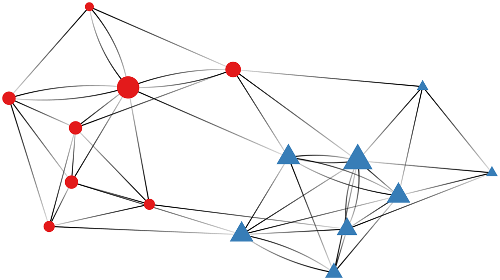
Figure 2. Higher-order dependence patterns in a network.

The visualization illustrates that actors belonging to the same group have a higher likelihood of interacting with each other, whereas interactions across groups are rarer. A prominent example of a network with this type of structure is discussed by Adamic and Glance (Reference Adamic and Glance2005), who visualize linkages between political blogs preceding the 2004 United States Presidential Election. Adamic and Glance (Reference Adamic and Glance2005) find that the degree of interaction between right- and left-leaning blogs is minimal and that most blogs are linked to others that are politically similar. This showcases the types of higher-order dependencies that can emerge in relational data. First, the fact that interactions are determined by a shared attribute, in this case political ideology, is an example of homophily. Homophily explains the emergence of patterns such as transitivity (“a friend of a friend is a friend”) and balance (“an enemy of a friend is an enemy”), which also have a long history in international relations. The other major type of meso-scopic features that emerge in relational data is community structure (Mucha et al., Reference Mucha, Richardson, Macon, Porter and Onnela2010), which is often formalized through the concept of stochastic equivalence (Anderson et al., Reference Anderson, Wasserman and Faust1992). Stochastic equivalence refers to a type of pattern in which actors can be divided into groups such that members of the same group have similar patterns of relationships. In the example above, each of the left leaning blogs would be considered stochastically equivalent to one another because any given left-leaning blog is more likely to interact with a blog of a similar political position and less likely to interact with one of a divergent political position.

These types of patterns frequently emerge in IR contexts.Footnote ³ For example, a perennial finding in the interstate trade literature emphasizes the role that geography plays in determining trade flows. Geographic proximity in the network context is an example of homophily—a shared attribute between actors that corresponds to a greater likelihood of the event of interest taking place. Alternatively, in the interstate conflict literature, we may find that actors who are each a member of a particular (formal or informal) alliance are likely to act similarly in the conflict network. Specifically, they will tend to initiate conflictual events with actors that their fellow alliance members initiate conflict with, and they will be unlikely to initiate conflict with the members of their alliance—an example of stochastic equivalence. In both these examples, we are able to explicitly parameterize the attribute that might explain the emergence of higher order dependence patterns. While sometimes the conditions driving these patterns, such as geography, are easy to identify, at other times it can be difficult to describe exactly why higher order dependence patterns in networks may develop.

3. Additive and multiplicative effect models for networks

To account for the dependencies that are prevalent in dyadic data, we turn to the AME model. The AME approach can be used to conduct inference on cross-sectional and longitudinal networks with binary, ordinal, or continuous linkages. It is flexible and easy to use for analyzing the kind of relational data often found in the social sciences. It accounts for nodal and dyadic dependence patterns, as well as higher-order dependencies such as homophily and stochastic equivalence.Footnote ⁴ The AME model combines the social relations regression model (SRRM) to account for nodal and dyadic dependencies and the latent factor model (LFM) for third-order dependencies.Footnote ⁵ For details on the SRRM see Li and Loken (Reference Li and Loken2002), Hoff (Reference Hoff2005), and Dorff and Minhas (Reference Dorff and Minhas2017). The AME model is specified as follows:

(2)$$\matrix{& y_{ij} = f( \theta_{ij}) ,\; \quad \hbox{where}\hfill \cr &\theta_{ij} = \beta_{d}^{\top} {\bf X}_{ij} + \beta_{s}^{\top} {\bf X}_{i} + \beta_{r}^{\top} {\bf X}_{\,j} \quad {( \rm Exogenous \; parameters) }\cr & \qquad + a_{i} + b_{\,j} + \epsilon_{ij} \quad {( \rm SRRM \; parameters) } \hfill\cr & \qquad+ {\bf u}_{i}^{\top} {\bf D} {\bf v}_{\,j} \quad {( \rm LFM \; parameters) }\hfill \cr }$$

where y _ij,t captures the interaction between actor i (the sender) and j (the receiver) at time t. We model a latent variable, θ _ij, first using a set of exogenous dyadic ($\beta _{d}^{\top } {\bf X}_{ij}$), sender ($\beta _{s}^{\top } {\bf X}_{i}$), and receiver covariates ($\beta _{r}^{\top } {\bf X}_{j}$). f is typically a mapping function, and can be one that applies to dichotomous, ordinal, or continuous distributions.

Next, to account for the dependencies that emerge in dyadic data that may complicate inference on the parameter associated with exogenous covariates, we add parameters from the SRRM and LFM. a _i and b _j in Equation 2 represent sender and receiver random effects incorporated from the SRRM framework:

(3)$$\matrix{ & \{ ( a_{1},\; b_{1}) ,\; \ldots,\; ( a_{n},\; b_{n}) \} {\rm iid}{\sim} N( 0,\; \Sigma_{ab}) \cr & \{ ( \epsilon_{ij},\; \epsilon_{\,ji}) \, \colon \, i \neq j\} {\hbox{iid}}{\sim} N( 0,\; \Sigma_{\epsilon}) ,\; \quad \hbox{where } \cr & \Sigma_{ab} = \left(\matrix{\sigma_{a}^{2} & \sigma_{ab} \cr \sigma_{ab} & \sigma_{b}^{2} }\right)\quad \Sigma_{\epsilon} = \sigma_{\epsilon}^{2} \left(\matrix{1 & \rho \cr \rho & 1 }\right)}$$

The sender and receiver random effects are modeled jointly from a multivariate normal distribution to account for correlation in how active an actor is in sending and receiving ties. Heterogeneity in the sender and receiver effects is captured by $\sigma _{a}^{2}$ and $\sigma _{b}^{2}$, respectively, and σ_ab describes the linear relationship between these two effects (i.e., whether actors who send [receive] a lot of ties also receive [send] a lot of ties). Beyond these first-order dependencies, second-order dependencies are described by $\sigma _{\epsilon }^{2}$ and a within dyad correlation, or reciprocity, parameter ρ.

The LFM contribution to the AME is in the multiplicative term: ${\bf u}_{i}^{\top } {\bf D} {\bf v}_{j} = \sum _{k \in K} d_{k} u_{ik} v_{jk}$. K denotes the dimensions of the latent space. The construction of the LFM here is actually quite similar to work on low rank approximations in computer science and has been applied to the development of recommender systems that companies like Amazon and Netflix use to model customer behavior (Resnick and Varian, Reference Resnick and Varian1997; Bennett and Lanning, Reference Bennett and Lanning2007).Footnote ⁶ This model posits a latent vector of characteristics u_i and v_j for each sender i and receiver j. The similarity or dissimilarity of these vectors will then influence the likelihood of activity, and provides a representation of third-order interdependencies. The LFM parameters are estimated by a process similar to computing the singular value decomposition (SVD) of the observed network. When computing the SVD we factorize our observed network into the product of three matrices: U, D, and V. This provides us with a low-dimensional representation of our original network.Footnote ⁷ Values in U provide a representation of how stochastically equivalent actors are as senders in a network or, for example, how similar actors are in terms of who they initiate conflict with. $\hat {{\bf u}}_{i} \approx \hat {{\bf u}}_{j}$ would indicate that actors i and j initiate battles with similar third actors. V provides a similar representation but from the perspective of how similar actors are as receivers. The values in D, a diagonal matrix, represent the levels of homophily in the network.Footnote ⁸ Note that this model easily generalizes to the case, common in IR, where interactions are undirected (e.g., the presence of conflict or a bilateral investment treaty). In the case of the SRRM, ρ is constrained to be one and instead of separate sender and receiver random effects a single actor random effect is utilized. For the LFM, an eigen-decomposition scheme is used to capture higher-order dependence patterns. In the application section, we show the applicability of the AME approach to both directed and undirected dyadic data. Parameter estimation in the AME takes place within the context of a Gibbs sampler in which we iteratively sample from the posterior distribution of the full conditionals for each parameter.Footnote ⁹

Non-iid observations in relational data result from the fact that there is a complex structure underlying the dyadic events or processes that we observe. Accounting for this structure is necessary if we are to adequately represent the data generating process. If one can specify each of the nodal, dyadic, and triadic attributes that influence interactions then the conditional independence assumption underlying standard approaches will be satisfied. However, it is rarely the case that this is possible even for TSCS data and thus modeling decisions must account for underlying structure. Failing to do so in either TSCS or dyadic data leads to a number of well-known challenges: (a) biased estimates of the effect of independent variables, (b) uncalibrated confidence intervals, and (c) poor predictive performance. Additionally, by ignoring these potential interdependencies, we often ignore substantively interesting features of the phenomena we investigate. The study of international relations is founded on the relations among actors. Why ignore the interdependencies that led to the study of IR in the first place?

4. Simulation study

We explore the utility of AME as an inferential tool for dyadic analysis via a simulation exercise.Footnote ¹⁰ Most scholars working with dyadic data are primarily concerned with understanding the effect of a particular independent variable on a dyadic-dependent variable. The goal of our simulation is to assess how well AME can provide unbiased and well-calibrated estimates of regression coefficients in the presence of unobserved dependencies, specifically, homophily. As discussed in the previous section, homophily is the idea that actors are more likely to have a tie if they have similar values on a particular variable, and in networks the presence of homophily can lead to third-order dependencies such as transitivity. Homophily can be operationalized by creating a dyadic covariate via the multiplication of a nodal covariate with its transpose. For example, if the nodal covariate was a binary indicator for democracy, multiplying it by its transpose would give us a dyadic covariate that represents whether any dyad is jointly democratic or not.Footnote ¹¹

Assume that the true data-generating process for a binary variable, Y, is given by:

(4)$$\eqalign{Z_{ij} & = \mu + \beta X_{ij} + \gamma W_{ij} + \epsilon_{ij},\; \quad \epsilon \sim normal( 0,\; 1) \cr Y_{ij} & = I( Z_{ij} > 0) }$$

X _ij = x × x ^T, where x is a nodal covariate that is drawn from a standard normal distribution. Similarly, W _ij = w × w ^T, where w is also a nodal covariate that is independently drawn from a standard normal distribution. We generate our binary dependent variable, Y, within a probit framework with Z serving as the latent variable. X and W are both dyadic covariates that are a part of the data-generating process for Y, but W is not observed. We compare inference for μ and β—the latter parameter would be of primary concern for applied scholars—using three models:

• • the “standard” international relations approach estimated through a generalized linear model;Footnote ¹²

• • the AME approach outlined in the previous section with a unidimensional latent factor space (K = 1);Footnote ¹³

• • and an “oracle” regression model that assumes we have measured all sources of dependencies and thus includes both x _ij and w _ij.

The first model corresponds to the “standard” approach in which little is explicitly done to account for dependencies in dyadic data. In the second model, we use the AME framework described in the previous section. For both the first and second models, we are simply estimating a linear model of X on Y, and assessing the extent to which inferences on the regression parameters are complicated by the presence of unobserved dependencies, W. In the last model, we provide an illustration of the ideal case in which we have observed and measured W and include it in our specification for Y. The oracle case provides an important benchmark for the standard and AME approaches.

For the simulation, we set the true value of μ (the intercept term) to − 2 and β (the effect of X on Y) to 1.Footnote ¹⁴ We conduct two sets of simulations, one in which the number of actors in the network is set to 50 and the other at 100. In total, we run 1000 simulations where we begin by simulating Y from the specification given in Equation 4 and then for each simulated Y we estimate a standard, AME, and oracle model.

We first compare the performance of the models in terms of how well they estimate the true values of μ and β in Figure 3. The panels on the left show the results for when the number of actors is set to 50 and on the right for 100 actors. The top pair of panels represents the estimates for μ while the bottom pair do the same for β. In each case, we find that the estimates for μ and β produced by the standard approach are notably off from their true values. On the other hand, the AME model performs just as well as the oracle at estimating the true parameter values.

Figure 3. Regression parameter estimates for the standard, AME, and oracle models from 1000 simulations. Summary statistics are presented through a traditional box plot, and the estimates from each simulation are visualized as well as points.

Next, we estimate the 95 percent credible interval for the three models in each of the simulations and estimate the proportion of times that the true value fell within those intervals. The results are summarized in Figure 4, and again we see that the AME approach performs as well as the oracle, while the standard approach performs poorly by comparison. The implication of the results presented in Figures 3 and 4 is that standard approaches can often fail at estimating parameter values and conducting inferential tasks in the presence of unobserved dependencies. The AME approach by comparison can be used as a tool for scholars working with dyadic data to still estimate the true effects of their main variables of interest, while accounting for dependencies that do often emerge in dyadic data.

Figure 4. Proportion of times the true value fell within the estimated 95 percent confidence interval for the standard, AME, and oracle models from 1000 simulations.

Moreover, the AME approach allows scholars to better understand what parameters their model may be missing. In the case of the simulation here, W is set as an unobserved dyadic covariate that has a homophilous effect on Y. The effect of W is homophilous within this framework because it is a dyadic attribute involving i and j that positively affects the degree to which actors interact with one another, i.e., y _ij. This type of unobserved dependency will be captured through the multiplicative effects portion of the model, ${\bf U}^{\top } {\bf D} {\bf V}$. To estimate how well the model performs, we recover the multiplicative effects term for each simulation and calculate the correlation between it and the unobserved dependency, W.Footnote ¹⁵ We visualize the distribution of the correlations from each of the 1000 simulations in Figure 5 for the case where the number of actors is set to 100 (top pair of panels) and 50. Additionally, we calculate the median across the correlations and display the result using a vertical line. For both n = 50 and n = 100, we find that the multiplicative effects perform very well in capturing the unobserved dependency, which indicates that the AME does not simply capture noise but also works as a tool to estimate unobserved structure.

Figure 5. Distribution of correlation between missing variable and multiplicative random effect in AME across the 1000 simulations. Vertical line through the distribution represents the median value across the simulations.

The simulation shows that beyond obtaining less biased and better-calibrated parameter estimates, a key benefit of the AME framework is to directly estimate unobserved dependencies through the random effects structure of the model. Scholars can use this framework in an iterative fashion: beginning with an estimated model, they can then empirically study the structure of the random effects to assess whether there are unobserved covariates that they want to include in their model. Importantly, this simulation underscores how a careful consideration of a systems’ interconnectedness, both through theoretical approaches and empirical models, can result in more precise estimates of direct and indirect effects across the system.

5. Applications with AME

We apply AME to three recent IR studies: Reiter and Stam (Reference Reiter and Stam2003), Weeks (Reference Weeks2012), and Gibler (Reference Gibler2017). Each of these studies use relational data of state interactions and propose both dyadic, monadic, and structural explanations for the behavior of actors in the system. We demonstrate the capabilities of AME with reference to existing studies in order to highlight several features of our network-based approach. First, we show that simply by using the AME framework scholars can better model the data generating process behind events of interest. Second, the results of AME estimation are interpretable alongside results using standard approaches. Third, through using this approach, we can also quantify the degree to which first-, second-, and third-order dependencies are present.

We obtain the data for these studies from their replication archives.Footnote ¹⁶ The chosen studies have each gained over 100 or more citations and were recently published.Footnote ¹⁷ Each of these articles are well-known and posit a hypothesis in which interdependencies are consequential. Reflecting the dominant approach in the literature, the studies test their hypothesis by employing some form of a GLM. Table 1 provides descriptive information for the studies that we replicate.

Table 1. Descriptive information about the replicated studies

For each of the studies listed above, we replicate the authors’ key model using their original estimation procedure, a GLM.Footnote ¹⁸ Next, utilizing the same covariate specifications, we estimate the models with the AME framework.Footnote ¹⁹ For Reiter and Stam (Reference Reiter and Stam2003) and Weeks (Reference Weeks2012), we use a version of AME that accounts for the directed nature of the data and for Gibler (Reference Gibler2017) we used an undirected version. In the directed formulation, separate random effects are used for senders and receivers in both the additive and multiplicative portions of the model.

A key claim that we have made is that by accounting for dependencies inherent to relational data, we can better capture the data generating process behind events of interest. To assess whether or not the AME approach successfully does this, we turn to an out-of-sample cross-validation strategy. An out-of-sample approach is essential since relying on in-sample procedures would enable models with more parameters, such as AME, to simply overfit the data. The cross-validation procedure is executed as follows. For each study, we randomly divide the data into k = 30 sets, letting s _ij,t be the set to which pair ij, t is assigned. Then for each s ∈ {1, …, k}, we estimate model parameters with {y _ij,t : s _ij,t ≠ s}, the data not in set s, and predict $\{ \hat {y}_{ij, t}\, \colon \, s_{ij, t} = s\}$ from these estimated parameters.

The result of this procedure is a set of sociomatrices ${{\hat Y}}$, in which each entry $\hat y_{ij, t}$ is a predicted value obtained from a subset of the data that does not include y _ij,t. Next we conduct a series of analyses to discern whether or not the AME model provides any benefit for each study. These analyses are summarized in Figure 6. The left-most plot in each of the panels evaluates performance using Receiver Operating Characteristic (ROC) curves. Models that have a better fit according to this metric will follow the upper-left corner border of the ROC space. In addition to ROC curves, we also use separation plots (Greenhill et al., Reference Greenhill, Ward and Sacks2011). Separation plots visualize each of the observations in the dataset according to their predicted probability. In this graph, the shaded panels correspond to the occurrence of an event. Darker panels are events, lighter panels are non-events. If a model performs well, then the events that actually occur would stack to the far right of the graph, where the predicted probabilities generated by the model are highest. The right-most plot in each of the panels evaluates performance using precision-recall (PR) curves. PR curves are useful in situations where correctly predicting events is more interesting than simply predicting non-events (Davis and Goadrich, Reference Davis and Goadrich2006). This is especially relevant in the context of our applications here, as they each are trying to model conflict within dyads, which is an infrequent occurrence.

Figure 6. Assessments of out-of-sample predictive performance using ROC curves, PR curves, and separation plots.

For each of the replications, we find that the AME approach substantially outperforms the original models in terms of out-of-sample predictive performance. This indicates that switching to the AME framework—even when using the same covariate specification as the original studies—enables scholars to better represent the data generating process of their events of interest. The fact that this analysis is done in an out-of-sample context ensures that the AME framework is not simply overfitting with more parameters. Instead, it suggests that the AME are capturing underlying structure previously missed by the exogenous covariates in the models.

Ignoring this underlying structure has consequences for inferential analysis.Footnote ²⁰ The fact that there is such a divergence in the performance of AME versus the original estimation procedures highlights that there are unobserved sources of bias in each of these studies. We hone in on the main finding of each study to draw into focus the potential consequences for ignoring these sources of bias and the inferential benefits of the AME estimation procedure. In Table 2, we present the overall results; the term Unconfirmed indicates that the statistical significance of the crucial finding in the original study is not found to hold in the AME estimation.Footnote ²¹

Table 2. Here we provide a brief summary of the key variable in each of the replications and a note about whether or not the highlighted finding remains when using our network-based approach

An important takeaway here is that many scholars are forced to make knowledge claims based on the statistical significance of a small set of covariates or the differences between these covariates. These differences may change dramatically once interdependencies are taken into account. This outcome follows from AME's ability to better account for the dependencies discussed in the previous section, whereas GLM approaches explicitly assume observational independence conditional on the specified covariates. As this is a widely-known limitation of GLM approaches, scholars often attempt to account for clustering of observations by including additional variables and adjusting the standard errors of the resulting estimates. At best, this method introduces noise and imprecision into results and at worst can produce misleading outcomes.

Next we discuss each of the replications in more detail and highlight the substantive insights drawn from the AME framework.

5.1. Reiter and Stam (Reference Reiter and Stam2003)

Reiter and Stam (Reference Reiter and Stam2003) examine the relationship between democracy, dictatorship, and the initiation of militarized disputes. Their work contests prior scholarship claiming that interstate dyads containing democracies and personalist dictatorships were particularly prone to conflict because of aggression on the part of the democratic state (Peceny et al., Reference Peceny, Beer and Sanchez-Terry2002). Using a directed dyadic dataset of almost a million observations, they find evidence against this hypothesis: dictators are in fact more likely to challenge democracies, but not the other way around. In addition, military regimes and single-party regimes are more prone to initiate disputes with democracies, but the opposite is not true.Footnote ²² As is prevalent in this literature, Reiter and Stam employ a logistic regression that includes an indicator of the time since the last dispute as well as three cubic splines. Based on their statistical analysis, they conclude that institutional constraints affect the propensity of democratic and non-democratic leaders to engage in military conflict.

The key variables in the original model measure whether or not the sender in the directed dyad is a personalist regime and the target a democratic regime (“Pers/Democ directed dyad”) or whether the opposite is true (“Democ/Pers directed dyad”). The authors find that coefficient of the Pers/Democ directed dyad indicator is positive, while the Democ/Pers directed dyad is too imprecisely measured to indicate a direction. In our re-estimation using the AME framework, we confirm these results, indicating that dictators are likely to initiate or engage in conflict with democratic regimes but not vice versa.

Even though we are able to confirm the original results, employing the AME model offers clear benefits in this case. As already shown in Figure 6, our approach performs notably better in reflecting the data generating process. The reason for this is that there is still underlying structure within this conflict system that the Reiter and Stam model does not fully capture. To highlight this we visualize the estimated sender random effects (a _i) from the SRRM portion of the AME framework in Figure 7.

Figure 7. Estimates of sender random effects (a _i) from AME for the Reiter and Stam (Reference Reiter and Stam2003) model. Positive values indicate that the particular country is more likely to be involved in conflict than predicted by the covariates in the model. Negative values indicate that the country is less likely to be involved in conflict. The left panel shows a _i estimates for all countries and right panel highlights the top ten countries in terms of positive and values of a _i.

The visualization of the sender random effects highlights that the behavior of countries does not fully accord with predictions from the covariates specified by Reiter and Stam. Specifically, we can see that countries such as Iraq, Israel, and Iran are more likely to be involved in initiating or continuing conflict with other countries than the model would predict. Further, other countries such as Sweden, Finland, and Swaziland are less likely to engage in conflict than the exogenous covariates in the model would suggest. In this case, the finding that countries in the middle east experience more conflict with other countries might lead one to more carefully examine the effects of geography on conflict initiation or to account for Colgan (Reference Colgan2010)'s theory that revolutionary petrostates are more aggressive. None of these findings change the key conclusion from Reiter and Stam's work, but by using the AME framework we are able to better understand the limitations of their model.

5.2. Weeks (Reference Weeks2012)

Weeks examines the influence of domestic institutions on the initiation of military conflicts by autocratic leaders. She argues that in some circumstances autocrats are held accountable for their foreign policy decisions, and that this is dependent on the audiences of autocrats. When the autocratic regime is nonmilitary, domestic audiences do not favor military actions, but in military autocracies this is not the case. Further, she argues that in personalistic regimes without a military or civilian domestic audience, the leaders are more likely to employ military force in their foreign policy. To study this question, Weeks employs a directed dyad design of conflict similar to that used by Reiter and Stam.

The major innovation in her study resides in the nuanced way she conceptualizes and codes regimes into four types: (a) Machine, (b) Junta, (c) Boss, and (d) Strongmen.Footnote ²³ She uses a logistic regression, following Beck et al. (Reference Beck, Katz and Tucker1998) and includes splines to capture temporal covariation in the dependent variable along with dyad clustered standard errors. The key findings of her work are that (a) juntas, boss, and strongmen regimes are more likely to initiate conflict than machine-type regimes and (b) machine-type regimes are no more belligerent than democracies.Footnote ²⁴ In the empirical analysis, Weeks finds that machines are less prone to initiate conflict than the reference category, whereas juntas, bosses, and strongmen are more conflict-prone. When analyzing the results using AME, however, we find that the parameters on each of her autocratic regime type variables are too imprecisely measured to draw any inference about their putative causal effects. Consequentially, none of the findings from her original analysis are confirmed once known dependencies among the data are taken into account via AME.

There is also a striking difference between Weeks’ original model and our estimation using AME in terms of capturing the data generating process. As with Reiter and Stam, the divergence is a result of the GLM framework's inability to account for underlying structure generating the event of interest. To uncover this structure, we illustrate another beneficial aspect of the AME framework, which is the multiplicative random effects estimated through the LFM portion of the model: ${\bf u}_{i}^{\top } {\bf D} {\bf v}_{j}$. These random effects account for higher order dependencies that manifest as a result of homophily and stochastic equivalence in dyadic data.

To visualize the multiplicative effects, we display the circular diagram shown in Figure 8. The nodes throughout the diagram represent countries and are colored according to their geographic position—a legend is provided in the center. The outer ring visualizes higher order dependence patterns through countries’ sender relationships—country positions here are estimated in the u_i random effects described in Equation 2. Countries that are more proximate to each other in this outer ring are more likely to send or initiate conflicts with similar targets. The inner ring, based on the estimates of v_i, is constructed such that countries closer together are more likely to receive conflict from the same sender countries. Last, the distance between countries in the inner and outer rings proportionately reflects who a country is more likely to be in conflict with.

Figure 8. Visualization of multiplicative effects for Weeks (Reference Weeks2012). Each circle designates a country and the color corresponds to the legend at the center of the visualization. Countries that cluster together in the outer ring are those that were found by the model to have similar sending patterns, meaning that they tend to send conflict to similar sets of countries. The inner ring clusters countries by the similarity of who they receive conflict from.

Figure 8 reveals a number of notable clusters. For example, in the bottom right corner we see the US, UK, Germany, Canada, and Israel. These states cluster together in the outer ring of this visualization because they tend to send conflicts to similar targets. Conversely, in the top left of the outer ring, we see a cluster of authoritarian countries: Iraq, Russia, Syria, North Korea, and China. We observe similar clusters in the inner ring. Specifically, we again see the US, UK, Germany, Canada, and Israel clustering together indicating that they are more likely to receive conflict from the same countries. The cluster of democratic and authoritarian countries facing each other in the inner and outer rings indicate that they are more likely to engage in conflict with one another.

Perhaps most critically, an evaluation of this visualization highlights Weeks’ original expectation of how states behave in the conflict system. Specifically, Iraq, Syria, Libya, and North Korea all fell under Weeks’ “boss” category, and each of these states tends to cluster together in the inner and outer rings. This indicates that even though we do not find support for Weeks’ assertion that certain authoritarian regime types are more likely to initiate conflict, we do find that these regimes are more likely to behave similarly in terms of who they target and receive conflict from.

5.3. Gibler (Reference Gibler2017)

The last replication we conduct with the AME model considers a study by Gibler (Reference Gibler2017). Gibler argues that the long-standing relationship between the relative parity of capabilities and initiation of militarized interstate disputes (MIDs) is almost completely mediated by the initial conditions for the members of the dyad when they joined the international system as sovereign members. In most specifications, after taking into account the initial conditions for dyadic entry, the statistical significance of power parity vanishes. This finding calls into question many IR theories about the role of balance in generating international conflict (Organski, Reference Organski1958).

To test this hypothesis, Gibler employs an undirected dyadic design and estimates his model using a GLM with dyad-clustered standard errors.Footnote ²⁵ With this design, Gibler finds support for both the insignificance of contemporary power parity, and the effect of the initial conditions for entry on driving conflict behavior. When we re-estimate using AME power parity still has a small, imprecisely measured effect, supporting Gibler's argument that contemporary power parity is an artifact of other aspects of state relations, and does not drive contemporary conflict behavior. At the same time, the AME approach finds that the effect of power parity when a country enters into the international system is too imprecisely measured to draw any inferences about its effect on the initiation of MIDs. Not only is our estimate of the effect of this variable small, but it has a very large relative standard error—over a magnitude larger than the parameter itself. Thus, while we can confirm the argument that the effect of power parity vanishes when accounting for both initial conditions and network dependencies, we find less support for the argument that initial conditions drive the initiation of MIDs.

In the two previous replications, we showed how to parse apart underlying structure using the SRM and LFM portions of the AME framework. Here we turn our focus to parameter interpretation in a substantive context. Specifically, even when the GLM and AME frameworks produce results that may seem to be in accordance with one another, the substantive interpretations of the effects of covariates can differ notably since the AME model uses a set of random effects to account for unobserved factors. To explore this, we focus on the effect of rivalry on MID initiation. Both the GLM and AME estimations find that rivalry has a positive effect on MID initiation, but the expected effects between the two models differ greatly.

To clarify the difference, we turn to a simulation-based approach. We employ mean or modal values for all independent variables, except we change the rivalry variable to indicate that there was a rivalry when the actual data suggest there is none. This provides us with two scenarios, one in which rivalry is set to one and the other zero, while in both scenarios all other parameters are set to their measure of central tendency. The expected values of this scenario are essentially a first difference plot comparing results with the model when estimated in two different ways: the GLM estimation and our AME approach.

As Figure 9 illustrates, the substantive results differ notably. The expected value of the dependent variable—the probability of the onset of a MID, is considerably lower once interdependencies are taken into account with the AME model. These are rare events, so the probabilities are low, but the difference in predictions is notable.

Figure 9. Marginal effects of a change in the Rivalry variable for both the AME and the Gibler estimation.