


1. Introduction
Electroconvection near an ion-selective surface is important in electrodialysis, desalination and rechargeable batteries with liquid electrolytes (Fleury, Chazalviel & Rosso Reference Fleury, Chazalviel and Rosso1993; Rubinstein, Zaltzman & Kedem Reference Rubinstein, Zaltzman and Kedem1997; Kim et al. Reference Kim, Ko, Kang and Han2010). This phenomenon is governed by strong couplings between electrostatic effects, fluid flow in the bulk region and the selective ion transport/reaction at the surface (Mani & Wang Reference Mani and Wang2020). So far, all previous studies on electroconvection have assumed infinitely fast ion transport across the surface so that the ions in solution are always in equilibrium with the adjacent electrode surface (Zaltzman & Rubinstein Reference Zaltzman and Rubinstein2007; Demekhin, Nikitin & Shelistov Reference Demekhin, Nikitin and Shelistov2013; Druzgalski, Andersen & Mani Reference Druzgalski, Andersen and Mani2013). However, experiments of electrodeposition on a metal surface in a dilute electrolyte shows that the current–voltage relation is strongly affected by the surface kinetics. Indeed, the reaction kinetics plays a key role in many flows of coupled transport and reaction, such as combustion (Williams Reference Williams1971) and CO $_2$ dissolution into a porous medium (Andres & Cardoso Reference Andres and Cardoso2011). To have a full understanding of electroconvection in real electrohydrodynamic systems, it is important to study the interaction between surface kinetics and electroconvection.
Caused by an electrohydrodynamic instability in a strong electric field (Rubinstein & Zaltzman Reference Rubinstein and Zaltzman2001; Rubinstein, Zaltzman & Lerman Reference Rubinstein, Zaltzman and Lerman2005), electroconvection enhances the mixing of the salt solution in the bulk region and generates the so-called ‘overlimiting current’. This phenomenon has been widely observed in various experimental settings, such as in microchambers connected by nanochannels (Kim et al. Reference Kim, Wang, Lee, Jang and Han2007; Yossifon & Chang Reference Yossifon and Chang2008; Abu-Rjal et al. Reference Abu-Rjal, Leibowitz, Park, Zaltzman, Rubinstein and Yossifon2019) and near an ion-selective membrane (Rubinstein et al. Reference Rubinstein, Manukyan, Staicu, Rubinstein, Zaltzman, Lammertink, Mugele and Wessling2008; de Valença et al. Reference de Valença, Wagterveld, Lammertink and Tsai2015) or a metal electrode surface (Fleury et al. Reference Fleury, Chazalviel and Rosso1993; Rubinstein et al. Reference Rubinstein, Manukyan, Staicu, Rubinstein, Zaltzman, Lammertink, Mugele and Wessling2008; Zhang et al. Reference Zhang, Warren, Li, Cheng, Han, Zhao, Liu, Deng and Archer2020). In all these examples, the surfaces are ion selective and only allow cations, for instance, to pass through or deposit, while blocking the anions because of the overlapping anion double layers inside the nanochannel or the interfacial chemistry of the metal electrode. In a strong electric field, the ions are fully depleted near the ion-selective surfaces generating a thin space charge layer outside the usual equilibrium double layer. Above a critical voltage, small perturbations of the ion concentration and electric field in the space charge layer grow and cause the electroconvective instability (Rubinstein & Zaltzman Reference Rubinstein and Zaltzman2000). This effect is very different from many other electrokinetic flows which may also be named as electroconvection. For example, the electrohydrodynamic instability may occur in an insulating fluid with unipolar charge injection (Lacroix, Atten & Hopfinger Reference Lacroix, Atten and Hopfinger1975), the deformation and instability of the interface between two weakly conducting and dielectric fluids are caused by the surface charge (Taylor Reference Taylor1966) and the conductance gradient (Lin et al. Reference Lin, Storey, Oddy, Chen and Santiago2004; Oddy & Santiago Reference Oddy and Santiago2005), and the electrohydrodynamic flow which generates colloidal assembly is directly related to the local change of ion conductance due to the colloids’ deposition on the electrode surface (Trau, Saville & Aksay Reference Trau, Saville and Aksay1997).
Through a linear stability analysis, Rubinstein and coworkers studied the instability of the quasi-electroneutral bulk region on a surface with no kinetic limitations (Rubinstein & Zaltzman Reference Rubinstein and Zaltzman2000, Reference Rubinstein and Zaltzman2001; Rubinstein et al. Reference Rubinstein, Zaltzman and Lerman2005). In this bulk analysis, they found that the second-kind electroosmotic slip velocity at the edge of the space charge layer is the key effect that causes the instability above a critical voltage. It predicts that the critical voltage for the onset of electroconvection is inversely proportional to the square root of the Péclet number. The other two effects, i.e. the first-kind slip velocity outside the equilibrium double layer as well as the bulk electroconvection due to charge density perturbations in the bulk region, do not generate instabilities by themselves in most realistic electrolytes (Zholkovskij, Vorotyntsev & Staude Reference Zholkovskij, Vorotyntsev and Staude1996; Lerman, Rubinstein & Zaltzman Reference Lerman, Rubinstein and Zaltzman2005). They marginally influence the critical voltage but do not qualitatively change the instability (Rubinstein et al. Reference Rubinstein, Zaltzman and Lerman2005). However, the bulk analysis underestimates the critical voltage for the onset of the electroconvection and it incorrectly predicts an infinite growth rate at infinite wavenumber. To overcome these issues, Zaltzman & Rubinstein (Reference Zaltzman and Rubinstein2007) performed a full analysis on the linear stability of the entire system, including the electroneutral bulk region, space charge layer and double layer. They found that the critical voltage predicted by the bulk analysis is lower than that predicted by the full analysis by approximately  $4\ln \delta$, where
  $\delta$ is the dimensionless double layer thickness normalized by the interelectrode distance. However, the source of this discrepancy was unclear. In this work, we will show that the difference results from a combination of the potential differences across the double layer and space charge layer. On a surface with finite reaction rate, the potential difference across the double layer increases and delays the onset of the electroconvective instability.
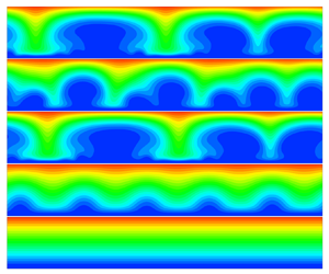
The nonlinear dynamics of electroconvective flows at high voltages has been studied through direct numerical simulations solving the Poisson–Nernst–Planck–Stokes equations. In a two-dimensional simulation, Pham et al. (Reference Pham, Li, Lim, White and Han2012) showed that the electric current exhibits hysteresis when changing the voltage. Demekhin and coworkers studied the time evolution of the electroconvection (Demekhin, Shelistov & Polyanskikh Reference Demekhin, Shelistov and Polyanskikh2011) and the dynamical transitions from limiting current to overlimiting current (Demekhin et al. Reference Demekhin, Nikitin and Shelistov2013). They showed that the onset of electroconvection is supercritical at small Péclet number and subcritical at high Péclet number. As one increases the voltage, the ion transport exhibits four regimes: one-dimensional (1-D) steady diffusion, steady electroconvection, periodic convection and chaotic motion. Druzgalski et al. (Reference Druzgalski, Andersen and Mani2013) analysed the statistics and the spatial/temporal spectra of electroconvection in these different regimes. Their simulations show that at a high voltage, the vortices strongly interact with the space charge layer and randomly generate short-time hot spots of high current density on the surface and therefore increase the mean current density. The three-dimensional simulations show similar results to the two-dimensional cases, with differences being quantitative rather than qualitative (Druzgalski & Mani Reference Druzgalski and Mani2016). More numerical simulations further investigated the influences of different effects on the electroconvection and ion transport, including an imposed flow (Kwak et al. Reference Kwak, Pham, Lim and Han2013; Pham et al. Reference Pham, Kwon, Kim, White, Lim and Han2016), the buoyancy force (Karatay et al. Reference Karatay, Andersen, Wessling and Mani2016), a patterned ion-selective surface (Davidson, Wessling & Mani Reference Davidson, Wessling and Mani2016), confinement by sidewalls (Andersen et al. Reference Andersen, Wang, Schiffbauer and Mani2017) and viscoelasticity due to polymer additives (Li, Archer & Koch Reference Li, Archer and Koch2019).
All previous studies so far have used the equilibrium boundary condition for ion concentration at the electrode–electrolyte interface. In reality, the reaction or passing rate of the ions on a surface is finite and interfacial kinetics is important. For instance, the exchange current density is 0.2–40  $\mathrm {mA}\ \mathrm {cm}^{-2}$ for lithium depending on electrolyte (Munichandraiah et al. Reference Munichandraiah, Scanlon, Marsh, Kumar and Sircar1994; Lopez et al. Reference Lopez, Pei, Oh, Wang, Cui and Bao2018) and 1–3
  $\mathrm {mA}\ \mathrm {cm}^{-2}$ for zinc and copper (Milora, Henrickson & Hahn Reference Milora, Henrickson and Hahn1973; Guerra et al. Reference Guerra, Kelsall, Bestetti, Dreisinger, Wong, Mitchell and Bizzotto2004), and the typical current density in experiments ranges from 0.1 to 10
  $\mathrm {mA}\ \mathrm {cm}^{-2}$. Therefore, the Damköhler number
  $Da$, which characterizes the ratio between the ion reaction and transport rates, ranges from 0.01 to 10. In Rubinstein et al. (Reference Rubinstein, Manukyan, Staicu, Rubinstein, Zaltzman, Lammertink, Mugele and Wessling2008) and Zhang et al. (Reference Zhang, Warren, Li, Cheng, Han, Zhao, Liu, Deng and Archer2020), electroconvection in dilute electrolytes is studied using copper and Nafion-covered zinc metal as the anode surface, respectively. The experiment of Rubinstein et al. (Reference Rubinstein, Manukyan, Staicu, Rubinstein, Zaltzman, Lammertink, Mugele and Wessling2008) is performed at a higher current density and observes smaller slopes in the current–voltage curves in both under- and overlimiting regimes and a delayed onset of overlimiting current than Zhang et al. (Reference Zhang, Warren, Li, Cheng, Han, Zhao, Liu, Deng and Archer2020). This result strongly suggests that in practical electrohydrodynamic cells, the surface kinetics has non-negligible influences on the electroconvective instability. Despite the strong experimental evidence of the effect of surface kinetics on electroconvection, this effect and the related flow field have not been studied in previous theoretical and simulation studies.
The Butler–Volmer (B–V) equation has been widely used to describe the non-equilibrium ion deposition on a metal surface (Bard et al. Reference Bard, Faulkner, Leddy and Zoski1980). The B–V equation is developed based on transition state theory considering both cathodic and anodic reactions, and it describes the dependence of the current flux on the electric potential drop across the interface (Bazant Reference Bazant2013). Although more sophisticated models, such as the electron transfer theory (Marcus Reference Marcus1956), have been developed to include more physical processes, the B–V condition is most commonly used for its simplicity and reasonable agreement with experiments. In steady electrodeposition on a metal surface, the linear stability analysis shows that B–V kinetics significantly affect the morphological instability in both underlimiting (Sundström & Bark Reference Sundström and Bark1995) and limiting (Nielsen & Bruus Reference Nielsen and Bruus2015a) current regimes. At the same wavenumber, the growth rate of an unstable mode increases with increasing Damköhler number. Through a phase-field simulation, Cogswell (Reference Cogswell2015) showed that the morphology of the long-time electrodeposition on a metal surface is directly controlled by the B–V kinetics at the interface. Depending whether the ion flux is reaction- or transport-limited, either smooth or dendritic electrodeposition can be observed in experiments for copper electrodeposition (Bai et al. Reference Bai, Li, Brushett and Bazant2016). So far, there has been no study to consider the effects of finite kinetic rates of the surface on electroconvection. The present study focuses primarily on the influence of surface kinetics on the instability of 1-D ion transport to a fixed surface, which is important for electrodialysis, desalination and planar electrodeposition in a liquid electrolyte. Additionally, we perform a linear stability analysis of a non-fixed surface to provide physical insight into the effects of electroconvective modes on the initial morphological evolution of an ion-depositing surface.
It is important to note that the B–V condition is applied at the edge of the bulk region and therefore is incompatible with the traditional equilibrium conditions of prescribed ion concentration or potential at the electrode–electrolyte interface. Since the exact microstructure of the interface is not fully understood, different boundary conditions derived from the B–V condition have been used in previous studies. Bazant, Chu & Bayly (Reference Bazant, Chu and Bayly2005) specified the electric potential drop by considering the capacitance of the Stern layer inside the diffusive double layer. In this method, the B–V condition is applied at the inner edge of the double layer instead of at the outer edge as in most studies. Chazalviel (Reference Chazalviel1990) and Nielsen & Bruus (Reference Nielsen and Bruus2015a) used a different boundary condition that assumes the depositing ion has zero gradient on the surface. This condition gives the same results for the 1-D ion transport as Bazant et al. (Reference Bazant, Chu and Bayly2005) with a specific Stern layer thickness and is more efficient in simulations since it avoids resolving the extremely thin double layer whose thickness is typically 0.1–1 nm. In some model experiments with extremely dilute salt concentration ( $\sim$1–10 mM), the double layer thickness can reach to approximately 3–10 nm. In this work, we extend the condition of Chazalviel (Reference Chazalviel1990) and Nielsen & Bruus (Reference Nielsen and Bruus2015a) to a more general case which is applicable for both underlimiting and overlimiting currents. As we will show later, neglecting the double layer does not qualitatively affect the linear instability or the nonlinear dynamics of the electroconvection. Nielsen & Bruus (Reference Nielsen and Bruus2015a) studied the linear morphological instability of a surface with finite reaction rate by focusing on the electroneutral region.
On many metal surfaces, electroconvection tends to enhance the variation of the surface topography by causing spatially and temporally varying ion fluxes and enhances the morphological instability (Fleury et al. Reference Fleury, Chazalviel and Rosso1993; Huth et al. Reference Huth, Swinney, McCormick, Kuhn and Argoul1995). This effect can be removed either by using a membrane to cover the surface or using a metal, such as zinc, whose planar electrodeposition is stable. As mentioned above, this work will mainly consider the pure electroconvection case without surface evolution. For the coupled electroconvective and morphological instabilities, most studies to date have only considered the early stage of surface evolution by conducting a linear stability analysis. The influence of B–V condition on the linear morphological variation of the metal surface has been studied by Nielsen & Bruus (Reference Nielsen and Bruus2015a). To understand the nonlinear surface development in a liquid electrolyte, full simulations with boundary-tracking techniques are required to capture the surface growth. Possible choices for such techniques include the phase-field method (Takaki Reference Takaki2014; Cogswell Reference Cogswell2015), level-set method (Gibou et al. Reference Gibou, Fedkiw, Caflisch and Osher2003), immersed boundary method (Griebel, Merz & Neunhoeffer Reference Griebel, Merz and Neunhoeffer1999) and the sharp interface model with a deforming grid (Nielsen & Bruus Reference Nielsen and Bruus2015b). In particular, Nielsen & Bruus (Reference Nielsen and Bruus2015b) studied the ramified growth of electrodeposition on a surface with the nonlinear B–V reaction model in the absence of electroconvection. They found that the dominant length scale of the deposition structures depends linearly on the most unstable wavelength obtained from a linear stability analysis.
In this work, we study the electroconvection in a liquid electrolyte near an interface with a finite reaction rate. The main goal is to understand the effects of finite kinetics on the hydrodynamics of pure electroconvection without dendritic growth. In addition, the morphological consequences of the electroconvection are studied using a linear stability analysis. In § 2, we describe the governing equations of the problem and the boundary conditions. The kinetics of the interface is described using the B–V condition. Section 3 shows the effects of the B–V condition on 1-D ion transport. The results are compared with the ones with traditional equilibrium conditions. In § 4, we study the linear instability of the 1-D transport using a spectral method. Both the purely electroconvective instability and its interaction with the morphological instability are considered. Theoretical analysis of the bulk region is also made and compared with the full analysis. In § 5, we perform a direct numerical simulation of the electroconvection near a fixed surface to study the effects of the interfacial kinetics on the nonlinear dynamics. Section 6 presents the summary and conclusion.
2. Governing equations and boundary conditions
As shown in figure 1, we consider a binary liquid electrolyte (valence  $\pm z$) between an ion-selective surface and a stationary reservoir. At high voltage, three regions are formed in the electrolyte, of which we resolve the space charge layer (micrometre thickness) and the electroneutral bulk region (millimetre thickness), but not the double layer (nanometre thickness). The governing equations are the Nernst–Planck equation for ion transport, the Poisson equation for the electric potential and the Stokes equation for the incompressible fluid. In dimensionless form, they are
 $$\begin{gather} \frac{\partial c^+}{\partial t} +Pe {\boldsymbol u}\boldsymbol{\cdot}\boldsymbol{\nabla} c^+ = \frac{1}{2(1-t_c)}[\nabla^2c^+ + \boldsymbol{\nabla}\boldsymbol{\cdot}(c^+\boldsymbol{\nabla}\varPhi)], \end{gather}$$
 $$\begin{gather}\frac{\partial c^-}{\partial t} +Pe {\boldsymbol u}\boldsymbol{\cdot}\boldsymbol{\nabla} c^- = \frac{1}{2t_c}[\nabla^2c^- - \boldsymbol{\nabla}\boldsymbol{\cdot}(c^-\boldsymbol{\nabla}\varPhi)], \end{gather}$$
 $$\begin{gather}-2\delta^2\nabla^2\varPhi=c^+ - c^-, \end{gather}$$
 $$\begin{gather}-\boldsymbol{\nabla} p+\nabla^2{\boldsymbol u} +{\boldsymbol f}_e=0, \end{gather}$$
 $$\begin{gather}\boldsymbol{\nabla}\boldsymbol{\cdot}{\boldsymbol u}=0, \end{gather}$$
where  $c^{\pm }$ are the concentrations of cation and anion,
  $\varPhi$ the electric potential,
  ${\boldsymbol u}$ the fluid velocity in a frame moving with the average speed of the evolving surface (on a fixed ion-selective surface, the frame is stationary),
  $p$ the pressure,
  ${\boldsymbol f}_e=\nabla ^2\varPhi \boldsymbol {\nabla }\varPhi$ the electric body force. Here
  $t_c=D^+/(D^++D^-)=0.5$ is the cation transference number,
  $D^+$ and
  $D^-$ are the diffusivities of cation and anion,
  $\delta =\sqrt {\varepsilon _r\varepsilon _0 RT/(2z^2F^2C_0)}/L$ is the dimensionless thickness of the electrical double layer,
  $L$ is the gap distance,
  $C_0$ is the bulk average ion concentration,
  $\varepsilon _r, \varepsilon _0, R, T, z$ and
  $F$ are the dielectric constant, vacuum permittivity, gas constant, temperature, valence of the ion and Faraday constant, respectively. The valence of the ion is set as
  $z=1$. The above equations are non-dimensionalized as follows: lengths by the gap distance
  $L$; velocity by
  $U_0=\varepsilon _r\varepsilon _0(RT)^2/(z^2F^2\eta L)$; time by
  $L^2/D_0$; ion concentration by
  $C_0$; and potential by
  $RT/zF$, where
  $\eta$ is the fluid viscosity and
  $D_0=2D^+D^-/(D^++D^-)$ is the average ‘salt’ diffusivity. The inertia term in the momentum equation is neglected because the Schmidt number
  $Sc=\eta /(\rho _0D_0)$ for ions in aqueous solutions is typically
  $O(10^3)$, where
  $\rho _0$ is the fluid density. The Péclet number
  $Pe =U_0L/D_0$ is independent of the electrolyte concentration. In this study, we set
  $Pe =0.5$ as in typical aqueous solutions unless otherwise specified. Linear stability analysis predicts that near an equilibrium ion-selective surface, the critical voltage for the onset of the electroconvection scales as
  $V_{cr}\sim Pe^{-1/2}$ (Rubinstein et al. Reference Rubinstein, Zaltzman and Lerman2005).

Figure 1. Schematic of the different regions (not drawn to scale) formed in an electrolyte near a fixed ion-selective surface of finite kinetics under an applied voltage  $V$. The double layer of nanometre thickness is not resolved. At high voltage, the electrolyte undergoes an electroconvective instability governed by the potential difference
  $V-\varPhi _s$, where
  $\varPhi _s$ is the interfacial potential at the inner edge of the space charge layer. For a non-fixed depositing surface such as metal electrode, the bottom boundary is subjected to a morphological perturbation.
Although the governing equations (2.1) for ion transport in a bulk fluid are well-understood, the appropriate boundary conditions are less clear and comprise substantial approximations. Here, we describe the boundary conditions at the boundary between the double layer and the bulk electrolyte or space charge layer. The adsorption of anions on the cation-selective surface ( $y=0$) is neglected and the first boundary condition is zero anion flux,
 \begin{equation} {\boldsymbol n}\boldsymbol{\cdot}(\boldsymbol{\nabla} c^{-} - c^{-}\boldsymbol{\nabla}\varPhi)=0, \end{equation}
where  ${\boldsymbol n}$ is the unit normal vector to the surface pointing into the electrolyte. The second condition at
  $y=0$ is the Butler-Volmer equation for the electrodeposition kinetics
 \begin{equation} I=2Da(c^+a_e^z\, \textrm{e}^{\alpha_c(\varPhi-Ca\kappa)}-a_m\, \textrm{e}^{-\alpha_a(\varPhi-Ca\kappa)}), \end{equation}
where  $I=|I^+_y(y=0)|$ is the dimensionless current density on the electrode surface,
  $I^+_y=\partial c^+/\partial y+c^+\partial \varPhi /\partial y$ is the cation flux in
  $y$-direction,
  $c^+$ is the cation concentration at the outer edge of the double layer which varies with the applied voltage,
  $a_e$ and
  $a_m$ are the activities of the electron and metal. Here we set
  $a_e=a_m=1$ and the valence of the ions
  $z=1$. The Damköhler number
 \begin{equation} Da=i_0/(2zFD^+C_0/L), \end{equation}
is the ratio between the exchange current density  $i_0$ and the limiting current. Here
  $\alpha _c$ and
  $\alpha _a=1-\alpha _c$ are the transfer coefficients for the cathodic and anodic reactions. Here
  $\kappa$ is the dimensionless curvature of the electrode surface,
  $Ca=\gamma \nu ^*_m/(LRT)$ is the capillary number of the depositing cation,
  $\kappa Ca$ represents the energy required to form a new surface. For lithium metal, the molar volume of the lithium is
  $\nu ^*_m=13.3\ \textrm {cm}^3\ \textrm {mol}^{-1}$,
  $\gamma =1.716\ \textrm {J}\ \textrm {m}^{-2}$ and
  $Ca=9.15\times 10^{-6}$. In (2.3), we have assumed the reference cation concentration is the same as the bulk average concentration
  $C_0$, and the standard electrode potential is zero since their specific values are not important in this study. The B–V condition is based on transition state theory for a one-step, one-electron process and includes both the cathodic and anodic reactions on the same electrode surface (Bard et al. Reference Bard, Faulkner, Leddy and Zoski1980). Recent studies show that the empirical B–V condition can be derived from more fundamental theories based on electron transfer (Rubi & Kjelstrup Reference Rubi and Kjelstrup2003) and non-equilibrium thermodynamics (Dickinson & Wain Reference Dickinson and Wain2020). Experimental measurements of the exchange current density and the transfer coefficients in the B–V equation have been conducted for different ions using various electrochemical techniques (Holze Reference Holze2007). Since the thickness of the double layer is very thin, the electrochemical reaction of the cations can be assumed to occur at the outer edge of the double layer instead of the metal or membrane surface. Both the potential
  $\varPhi$ and the cation concentration
  $c^+$ vary with the applied voltage. As
  $Da\to \infty$, (2.3) reduces to the equilibrium condition
  $\ln c^++\varPhi -Ca\kappa =0$, which is also consistent with the traditional boundary conditions
  $c^+=1$ and
  $\varPhi =0$ at
  $y=0$ if one neglects the surface tension. Other constant values of
  $c^+$ at
  $y=0$ used in previous studies can also be recovered by choosing different values of the reference concentrations and potentials in (2.3).
If one only considers the quasi-electroneutral bulk region of  $c^+=c^-=c$, the boundary conditions (2.2) and (2.3) are sufficient to solve the reduced Nernst–Planck–Poisson equations
  $\partial c/\partial t+Pe {\boldsymbol u}\boldsymbol {\cdot }\boldsymbol {\nabla } c=\nabla ^2 c$ and
  $(1-2t_c)\nabla ^2 c=\boldsymbol {\nabla }(c\boldsymbol {\nabla }\varPhi )$. However, to consider the non-electroneutral space charge layer, a third boundary condition is required. Here, we assume the cation and anion have the same gradient at the surface,
 \begin{equation} {\boldsymbol n}\boldsymbol{\cdot}\boldsymbol{\nabla} c^{+} = {\boldsymbol n}\boldsymbol{\cdot}\boldsymbol{\nabla} c^-, \end{equation}
which is similar to the condition in Chazalviel (Reference Chazalviel1990) and Nielsen & Bruus (Reference Nielsen and Bruus2015a) but here it is applied for both the under- and over-limiting current regimes. The above condition also gives the same base state solution as Bazant et al. (Reference Bazant, Chu and Bayly2005) for a specific Stern layer thickness. It is more efficient in simulations since it avoids resolving the extremely thin double layer. At a small current, (2.5) applies at the edge of the bulk region and recovers the quasi-electroneutrality condition. At a high enough current, when the anion is fully depleted near the surface, condition (2.5) leads to a zero cation gradient at the inner edge of the space charge layer. This condition enables us to precisely define the cation concentration and the electric potential at the edge of the double layer. Note that the concentration yielding a thin double layer ( $\sim$3 nm at 10 mM) is much lower than the concentration having strong effects of finite ion size and ion–ion interactions (100–1000 M). These effects are typically important in ionic liquids and are better described by the modified Nernst–Planck–Poisson models (Bockris & Reddy Reference Bockris and Reddy1998; Bazant, Storey & Kornyshev Reference Bazant, Storey and Kornyshev2011; Wang et al. Reference Wang, Bao, Pan and Sun2017). In a relatively dilute electrolyte, the effects of a non-ideal solution are negligible, meanwhile the condition of a thin double layer is still valid.
For the fluid, we use the no-penetration and no-slip boundary condition at  $y=0$,
 $$\begin{gather} \frac{\nu_m}{\nu_m-\nu_c}{\boldsymbol n}\boldsymbol{\cdot}{\boldsymbol u} =\frac{1}{Pe}\frac{\partial h}{\partial t} =\frac{\nu_m}{2Pe(1-t_c)}(i-i_{1D}), \end{gather}$$
 $$\begin{gather}(\boldsymbol{\mathsf{I}}-{\boldsymbol n}{\boldsymbol n}) \boldsymbol{\cdot}{\boldsymbol u}=0, \end{gather}$$
where  $h$ is the perturbation of the interface height,
  $i$ is the local current,
  $i_{1D}$ is the 1-D base state current, and
  $\boldsymbol{\mathsf{I}}$ is the identity matrix. On a fixed surface,
  $\partial h/\partial t=0$ and the fluid normal velocity is zero. Note that the above conditions only keep the leading-order terms in the Taylor expansion of the velocity at the anode surface. The Péclet number appears here due to the non-dimensionalization,
  $\nu _m=\nu ^*_mC_0$ and
  $\nu _c=\nu ^*_cC_0$ are the dimensionless partial molar volumes of the metal atom and the cation in the electrolyte solution. Here, the expression is based on the volume average velocity and has a different prefactor than that derived for the mass average velocity in Sundström & Bark (Reference Sundström and Bark1995). We choose to use the volume average velocity because it is divergence-free for a solution with additive partial molar volumes (Brenner Reference Brenner2005a) even though the mass density changes with ion concentration. Brenner (Reference Brenner2005b) has also suggested that the velocity appearing in the deviatoric stress tensor should be the volume average velocity. The exact partial molar volume of the cation is difficult to measure in experiments because the cation and anion are added simultaneously to the solution. Marcus & Hefter (Reference Marcus and Hefter2004) studied sequences of salts with the same anion and different cations and assumed the partial molar volume of the largest cation was the same as its van der Waals volume. It was then inferred that small ions such as lithium have very small partial molar volumes, because the change of volume of the solvent nearly cancels the volume of the cation itself. Thus, we assume
  $\nu _c=0$ in this study. Nevertheless, the exact value of
  $\nu _c$ has a small effect on the final results for the morphological instability. Equations (2.2)–(2.6) form the full boundary conditions at
  $y=0$. In comparison, the traditional equilibrium boundary conditions at
  $y=0$ are
  $c^+=1, \varPhi =0$, and (2.2), (2.6).
On the other side, at  $y=1$, we assume the liquid electrolyte is under equilibrium conditions. The boundary conditions include fixed cation/anion concentration, fixed electric potential
 \begin{equation} c^+ = c^- = 1, \quad \varPhi=V, \end{equation}
and the no-slip condition  ${\boldsymbol u}=0$. Compared with the no-slip condition, Druzgalski et al. (Reference Druzgalski, Andersen and Mani2013) also used the stress-free condition at
  $y=1$ assuming it is at the boundary of the fully mixed electrolyte. This difference has minor effects on the results since electroconvection mainly occurs near the bottom surface.
In typical experiments with aqueous electrolytes, the half-interelectrode distance is around 1 mm, the double layer thickness ranges from 0.1–10 nm, the dynamic viscosity  $\eta =10^{-3}\ \textrm {Pa}\,\textrm {s}$, the dielectric constant of water
  $\varepsilon =80$, the ion diffusivity
  $10^{-9}\ \textrm {m}^2\ \textrm {s}^{-1}$, the ion concentration
  $C_0=0.01$–
 $1$ M, the exchange current density
  $i_0=10^{-2}$–
 $10\ \textrm {mA}\ \textrm {cm}^{-2}$ and the applied voltage up to 4 Volts. Based on these parameters, we choose
  $Pe=0.5, \delta =10^{-6}$–
 $10^{-3}, V=20$–
 $100$ and
  $Da=10^{-3}$–
 $\infty$ for this study.
3. 1-D ion transport
To compare the B–V condition with the traditional boundary condition, we first consider the 1-D version of (2.1) for steady diffusion and migration
 $$\begin{gather} \frac{\partial c^+}{\partial y}+c^+\frac{\partial\varPhi}{\partial y}=I, \end{gather}$$
 $$\begin{gather}\frac{\partial c^-}{\partial y}-c^-\frac{\partial\varPhi}{\partial y}=0, \end{gather}$$
 $$\begin{gather}-2\delta^2\frac{\partial^2\varPhi}{\partial y^2}=c^+ - c^-, \end{gather}$$
with boundary conditions (2.2)–(2.5) and (2.7a,b).
In the limit of zero space charge layer thickness, the current is
 \begin{equation} I=2Da[\textrm{e}^{\alpha_c V}(1-I/2)^{1+\alpha_c} - \textrm{e}^{-\alpha_a V}(1-I/2)^{-\alpha_a}]. \end{equation}
As  $Da\to \infty$, (3.2) recovers the classical relation
  $I=I_{lim}(1- \textrm {e}^{-V/2})$ with the limiting current density
  $I_{lim}=2$ at zero space charge layer thickness (Rubinstein & Zaltzman Reference Rubinstein and Zaltzman2000).
For the electroneutral bulk region with  $c^+=c^-=c$, the ion concentration and potential are
 \begin{equation} c^\pm = c=\frac{I}{2}(y-1)+1, \quad \varPhi=\ln c+V. \end{equation}
At the interface  $y=0$, the ion concentration is
  $c_s=1-I/2$ and the electric potential jump is
  $\varPhi _s=\ln c_s+V$. Using (3.3a,b), the current can be written in a form which only depends on the potential drop across the electrolyte
 \begin{equation} I=2(1- \textrm{e}^{-(V-\varPhi_s)}). \end{equation}
This expression is derived from the zero-flux condition of anion (or constant electrochemical potential of anion) and the electroneutral condition, and removes the effects of the interfacial kinetics. Equations (3.2) and (3.4) give the current at leading order for small  $\delta$. More discussion on the high-order corrections on the current can be found in Rubinstein & Zaltzman (Reference Rubinstein and Zaltzman2001), Ben & Chang (Reference Ben and Chang2002) and Yariv (Reference Yariv2009).
Figure 2( $a$) shows the current–potential curves at different Damköhler numbers for
  $\delta =10^{-3}$. The current monotonically increases with the applied voltage and it has two regimes, the underlimiting current regime at low voltage, and the limiting current regime with a smaller slope at high current. Although this is not shown in the figure, the slope of the limiting current decreases with decreasing
  $\delta$ and it approaches the asymptotic solution (3.2) as
  $\delta \to 0$. At the same voltage, the influence of the B–V kinetics on the current also has two regimes. In the underlimiting regime, the current is strongly affected by
  $Da$, while at the limiting current, the influence is much weaker. As
  $Da\to \infty$, the B–V condition agrees well with the traditional equilibrium condition, the difference further decreases at smaller double layer thickness. Figure 2(
 $b$) shows that the current only depends on the potential drop
  $V-\varPhi _s$ across the bulk electrolyte.

Figure 2. The current for steady 1-D ion transport as a function of ( $a$) the applied total voltage
  $V$ and (
 $b$) the voltage across the electrolyte
  $V-\varPhi _s$ at
  $\delta =10^{-3}$. The results for the B–V conditions (coloured lines) overlay with each other.
Figure 3 shows the profiles of the ion concentrations and potential at  $V=2$ and 20 obtained using the two boundary conditions. The results for the traditional equilibrium condition have been shown in many previous studies. At small voltage, the electrolyte has two regions, the electroneutral bulk and the thin double layer. At high voltage, the space charge layer is formed outside the double layer. In the bulk region, the ion concentration and potential have linear and logarithmic profiles, respectively. With the new boundary condition (2.3) and (2.5), the double layer is replaced by a jump condition at
  $y=0$, while the space charge layer and the bulk region remain similar to the ones obtained using the equilibrium condition. The differences between the two results would be further reduced by decreasing
  $\delta$.

Figure 3. ( $a$) The ion concentrations (red,
  $c^+$; blue,
  $c^-$) and (
 $b$) potential
  $\varPhi$ profiles for the 1-D steady ion transport,
  $\delta =10^{-3}$.
The interfacial properties at  $y=0$ are important since they directly control the ion transport through the B–V condition. For underlimiting currents, the ion concentrations
  $c^\pm _s=c_s$ and the potential jump
  $\varPhi _s$ are directly determined by (3.3a,b) at
  $y=0$,
 $$\begin{gather} c_s=1-Da(\textrm{e}^{\alpha_c V}c_s^{1+\alpha_c}-\textrm{e}^{-\alpha_a V}c_s^{-\alpha_a}), \end{gather}$$
 $$\begin{gather}e^V-\textrm{e}^{\varPhi_s}=Da(\textrm{e}^{(1+\alpha_c)\varPhi_s}-\textrm{e}^{V-\alpha_a\varPhi_s}), \end{gather}$$
which satisfies  $\varPhi _s=\ln c_s+V$. At the limiting current, the above equation predicts
  $c_s\to 0$ and
  $\varPhi _s\to V/2$. However, in reality a space charge layer will be formed near the electrode where the anion is fully depleted at
  $y=0$ while the cation retains a small but non-zero concentration. Assuming that ion migration dominates over diffusion inside the space charge layer, the thickness of the space charge layer
  $\delta _s$, the cation concentrations
  $c^+_s, c^-_s$ and the potential
  $\varPhi _s$ at the interface are
 $$\begin{gather} \delta_s=\left(\frac{9\delta^2(V-\varPhi_s)^2}{8}\right)^{1/3}, \end{gather}$$
 $$\begin{gather}c^+_s=c_s=\frac{\sqrt{2}\delta}{\sqrt{\delta_s}} =\left(\frac{8\delta^2}{3(V-\varPhi_s)}\right)^{1/3}, \quad c^-_s=0, \end{gather}$$
 $$\begin{gather}c_s\, \textrm{e}^{\varPhi_s}-\frac{1}{Da}\, \textrm{e}^{\alpha_a\varPhi_s}=1. \end{gather}$$
The above results are similar to those of Chazalviel (Reference Chazalviel1990), except that here we use  $V-\varPhi _s$ instead of
  $V$ for the potential drop. For
  $Da\to \infty$, the potential jump recovers the equilibrium condition for the chemical potential of the cation
  $\varPhi _s+\ln c_s=0$. At a high voltage, the right-hand side of (3.6c) is negligible and
  $\varPhi _s\approx -\ln (Dac_s)/\alpha _c$. In the next section, (3.6a) is needed to consider the morphological instability of a surface with B–V kinetics at the limiting current.
Figures 4( $a$) and 4(
 $b$) compare the numerical and asymptotic results for
  $c^\pm _s$ and
  $\varPhi _s$ as functions of
  $V$. For the simulations with (2.3) and (2.5), they can be directly determined at
  $y=0$, and for simulations with equilibrium boundary conditions, we take the minimum
  $c^+$ as
  $c_s$ and the corresponding potential as
  $\varPhi _s$ (see figure 3). The asymptotic solutions (3.5a) and (3.6a) agree with the numerical results in both underlimiting and limiting current regimes. At smaller
  $Da$, the slower interfacial kinetics delay the transition between the two regimes. Nevertheless, once the space charge layer is formed, the cation concentration
  $c_s$ at the inner boundary of the space charge layer becomes independent of
  $Da$. The equilibrium condition predicts similar results for
  $c_s$, while it greatly overestimates
  $\varPhi _s$ in the limiting current regime due to the rapid variation of the potential inside the space charge layer. In figures 4(
 $c$) and 4(
 $d$), we compare the thickness of the space charge layer
  $\delta _s$ obtained using different boundary conditions. For the calculations shown,
  $\delta _s$ is defined as the position of the local maximum space charge density
  $\rho =c^+-c^-$. We also calculated
  $\delta _s$ by extending the linear bulk concentration and determining its intercept with the
  $x$-axis. The difference between the two results is around
  $1\,\%$. The two numerical results and the asymptotic solution (3.6a) agree with each other, particularly at small double layer thickness.

Figure 4. The effects of the boundary condition, double layer thickness  $\delta$ and Damköhler number on the variations of (
 $a$) the ion concentrations
  $c^\pm _s$, (
 $b$) potential
  $\varPhi _s$ at the interface and (
 $c,d$) the thickness of the space charge layer
  $\delta _s$ with the applied voltage
  $V$ for 1-D transport.
4. Linear instability
In this section, we discuss the linear instability of the 1-D ion transport described in the last section. Depending on whether the surface is fixed or allowed to evolve with ion deposition, the instability can either be purely electroconvective or include morphological instability. We use two methods to solve the instability problem. In the full analysis, which considers both the quasi-electroneutral bulk region and the space charge layer, we numerically solve the eigenvalue problem using the ultraspherical spectral method (Olver & Townsend Reference Olver and Townsend2013). In the bulk analysis, we only consider the instability in the bulk region and the space charge layer is replaced by an electroosmotic slip velocity proposed by Rubinstein and coworkers (Rubinstein et al. Reference Rubinstein, Zaltzman and Lerman2005; Zaltzman & Rubinstein Reference Zaltzman and Rubinstein2007). In the next subsection, we will first study the purely electroconvective instability using these two methods.
4.1. Purely electroconvective instability
For the purely electroconvective instability, the electrolyte–electrode interface is fixed,  $h=\kappa =0$. The ion concentration, electric potential and velocity are perturbed as
  $c^\pm =c^\pm _0+c^\pm _1(y)\, \textrm {e}^{\textrm {i}kx+\sigma t}, \varPhi =\varPhi _0+\varPhi _1(y)\, \textrm {e}^{\textrm {i}kx+\sigma t}$, and
  ${\boldsymbol u}={\boldsymbol u}_1(y)\, \textrm {e}^{\textrm {i}kx+\sigma t}$. Here
  $c^\pm _0, \phi _0$ are the base state solution obtained from (3.1a),
  $c^\pm _1, \varPhi _1$ and
  ${\boldsymbol u}_1$ are the perturbed variables governed by
 $$\begin{gather} \sigma c^+_1+Pe\, v_1c_0^{+\prime} =\frac{1}{2(1-t_c)}[c^{+\prime\prime}_1 -k^2c^+_1-k^2c^+_0\varPhi_1+(c^+_0\varPhi_1'+c^+_1\varPhi_0')'], \end{gather}$$
 $$\begin{gather}\sigma c^-_1+Pe\, v_1c_0^{-\prime} =\frac{1}{2t_c}[c^{-\prime\prime}_1 -k^2c^-_1+k^2c^-_0\varPhi_1-(c^-_0\varPhi_1'+c^-_1\varPhi_0')'], \end{gather}$$
 $$\begin{gather}2\delta^2(\varPhi_1''-k^2\varPhi_1)=c^-_1-c^+_1, \end{gather}$$
 $$\begin{gather}v_1^{(4)}-2k^2v_1''+k^4v_1=k^2((\varPhi_1''-k^2\varPhi_1)\varPhi_0'- \varPhi_1\varPhi_0^{(3)}). \end{gather}$$
The governing equations above are the same as those studied by Rubinstein et al. (Reference Rubinstein, Zaltzman and Lerman2005) and Zaltzman & Rubinstein (Reference Zaltzman and Rubinstein2007). The perturbed boundary conditions are, at  $y=0$,
 $$\begin{gather} c_1^{-\prime}-c_0^-\varPhi_1'-c_1^-\varPhi_0'=0, \end{gather}$$
 $$\begin{gather}c_1^{+\prime}+c_0^+\varPhi_1'+c_1^+\varPhi_0' =2Da[(c^+_1+c^+_0\alpha_c\varPhi_1)\, \textrm{e}^{\alpha_c\varPhi_0} +\alpha_a\varPhi_1\, \textrm{e}^{-\alpha_a\varPhi_0}], \end{gather}$$
 $$\begin{gather}c_1^{+\prime}-c_1^{-\prime}=0, \end{gather}$$
 $$\begin{gather}v_1=v_1'=0, \end{gather}$$
and at  $y=1$,
 \begin{equation} c_1^+ = 0, \quad c_1^- = 0, \quad \varPhi_1=0, \quad v_1=v_1'=0. \end{equation}
In the limit  $Da\to \infty$, the perturbed B–V kinetic boundary condition reduces to
  $c^+_1+c^+_0\varPhi _1=0$ by applying
  $\ln c^+_0+\varPhi _0=0$ at
  $y=0$.
Both the base state (3.1a) and the perturbed (4.1) are solved using the ultraspherical spectral method (Olver & Townsend Reference Olver and Townsend2013). Unlike the classical Chebyshev collocation method, this method constructs the matrices in the coefficient space and uses banded operators to generate a well-conditioned generalized eigenvalue problem. Therefore, it is capable of solving eigenvalue problems with thin boundary layers. The electroconvective instability in an electrolyte bounded by surfaces with two different boundary conditions, the B–V kinetic condition with  $Da\to \infty$ and the traditional equilibrium condition, are also compared. The neutral stability curves show that resolving the thin double layer decreases the critical voltage by a constant value independent of wavenumber. Detailed comparisons are given in the Appendix.
Figure 5( $a$) shows the neutral stability curves in the
  $k-V$ space at different
  $Da$ predicted by the full analysis. The double layer thickness is
  $\delta =10^{-3}$. As
  $Da\to \infty$, the critical voltage is
  $V_{cr}=22.02$ and the corresponding wavenumber is
  $k_{cr}=4.78$. With decreasing
  $Da$, the critical voltage monotonically increases, while
  $k_{cr}$ is not affected. In figure 5(
 $b$), all the neutral stability curves collapse well when plotted with
  $V_{cr}-\varPhi _s$, showing that the electroconvective instability is insensitive to the potential drop across the double layer. As we will see in the following, this is because the electroosmotic slip velocity which causes the instability is driven by the potential drop across the bulk electrolyte.

Figure 5. The neutral stability curves plotted in terms of ( $a$)
$a$)  $V$ and (
 $b$)
$b$)  $V-\varPhi _s$ versus the wavenumber
  $k$ for the electroconvective instability at different
  $Da$ predicted by the full analysis,
  $\delta =10^{-3}$.
To further understand the effects of interfacial kinetics on the electroconvective instability, we consider the linear instability of the quasi-electroneutral bulk region where  $c^+=c^-=c$. In most realistic electrolytes, the electroconvective instability occurs only at the limiting current and is caused by the second-kind electroosmotic slip velocity at the edge of the space charge layer. Following Rubinstein et al. (Reference Rubinstein, Zaltzman and Lerman2005), we introduce the electrochemical potential of the anion
  $\mu =\ln c-\varPhi$ to simplify the equations. The details of the linear stability analysis in the bulk region can be found in Rubinstein et al. (Reference Rubinstein, Zaltzman and Lerman2005). Here we only summarize the main results. The base state solutions (3.3a,b) are
 \begin{equation} c_0=1+\frac{I}{2}(y-1), \quad \mu_0= - V, \end{equation}
where  $I=2$ in the limiting current regime. Noticing
  $\mu _1=c_1/c_0-\varPhi _1$, the perturbed equations can be written as
 $$\begin{gather} \sigma c_1+Pe\, c_0'v_1 =c^{\prime\prime}_1 -k^2c_1, \end{gather}$$
 $$\begin{gather}\sigma c_1+Pe\, c_0'v_1 =\frac{1}{2t_c}[(c_0\mu_1')^{\prime} -k^2c_0\mu_1], \end{gather}$$
 $$\begin{gather}v_1^{(4)}-2k^2v_1''+k^4v_1=0, \end{gather}$$
which are exactly the same as the corresponding equations in Rubinstein et al. (Reference Rubinstein, Zaltzman and Lerman2005). At  $y=0$, the perturbed boundary conditions (2.2), (2.3) and (2.6) become
 $$\begin{gather} c_1=0, \quad \mu_1'=0, \quad v_1=0, \end{gather}$$
 $$\begin{gather}v_1'=V^*k^2\left(\mu_1-\frac{c_1'}{c_0'}\right) -\frac{1}{8}V^{*2}k^2 \frac{c_1'}{c_0'}. \end{gather}$$
At  $y=1$, the boundary conditions are
 \begin{equation} c_1=0, \quad \frac{c_1}{c_0}-\mu_1=0, \quad v_1=v_1'=0. \end{equation}
Note that in (4.6a), the condition  $c_1=0$ at
  $y=0$ is due to the full depletion of the ions at the edge of the bulk region at the limiting current. In the condition (4.6b),
  $V^*=V-\varPhi _s+\frac {2}{3}\ln \delta$ where
  $\varPhi _s$ is the potential jump across the double layer. The term
  $\frac {2}{3}\ln \delta$ is the characteristic potential difference across the space charge layer, whose thickness scales as
  $\delta ^{2/3}$ and wherein the potential roughly follows the same logarithmic profile as the bulk region. Rubinstein & Zaltzman (Reference Rubinstein and Zaltzman2001) also derived this term for the slip velocity (their (2.102)) but later neglected it by assuming
  $V\gg |\ln \delta |$ although this limit is not typically achieved in practice. Here, we use the simple estimation of the potential difference in the space charge layer to improve the quantitative prediction of the bulk analysis. The slip velocity (4.6b) has the same expression as Reference Rubinstein, Zaltzman and LermanRubinstein et al.'s (Reference Rubinstein, Zaltzman and Lerman2005) (203), it includes the contributions from both the first-kind (
 ${\sim}V^*$) and the second-kind slip velocities (
 ${\sim}V^{*2}$). The second-kind slip velocity is caused by the tangential variation of the normal ion concentration gradient and it is the dominant effect that causes the electroconvective instability. The first-kind slip velocity is caused by the tangential variation of the voltage and it slightly increases the critical voltage for the onset of the electroconvective instability. More systematic discussion on the structures and the potential drops in the equilibrium and non-equilibrium double layers as well as the unified asymptotic description of the thin layers can be found in Zaltzman & Rubinstein (Reference Zaltzman and Rubinstein2007).
In the bulk analysis, the linear instability is affected by the B–V kinetics only through the slip velocity (4.6b), and the results are the same as those in Rubinstein et al. (Reference Rubinstein, Zaltzman and Lerman2005) except that  $V$ is replaced by
  $V^*$. The critical voltage for the onset of the electroconvective instability is determined by the modes with large wavenumbers (
 $k\gg 1$),
 \begin{equation} V_{cr}=V^*_{cr}+\varPhi_{s,cr}-\tfrac{2}{3}\ln\delta, \end{equation}
where
 \begin{equation} V^*_{cr}=4\left(\sqrt{\frac{2}{Pe}+\left(\frac{8t_c}{3}-1\right)^2} +\frac{8t_c}{3}-1\right), \end{equation}
is the same as Rubinstein et al. (Reference Rubinstein, Zaltzman and Lerman2005) (207). Without the first-kind slip velocity, it reduces to the well known expression  $V^*_{cr}=4\sqrt {2/Pe}$ (Rubinstein & Zaltzman Reference Rubinstein and Zaltzman2000). The Damköhler number
  $Da$ is embedded in
  $\varPhi _{s,cr}$ by solving (3.6a) with
  $V=V_{cr}$ at the limiting current. The above result agrees with the full analysis prediction that the onset of the electroconvective instability occurs at a value of
  $V-\varPhi _s$ that is independent of
  $Da$.
$Da$.
At small  $Da$,
$Da$,  $\varPhi _s\approx -\ln (Dac_s)/\alpha _c$ and (4.8) can be simplified as
 \begin{equation} V_{cr}-\frac{1}{3\alpha_c}\ln V_{cr} =V^*_{cr}-\frac{1}{\alpha_c}\ln Da-\frac{2(1+\alpha_c)}{3\alpha_c}\ln\delta -\frac{1}{3\alpha_c}\ln\frac{8}{3}, \end{equation}
showing that the critical voltage increases logarithmically with decreasing  $Da$. As
  $Da\to \infty$, the critical voltage
 \begin{equation} V_{cr}-\tfrac{1}{3}\ln
V_{cr}=V^*_{cr} -\tfrac{4}{3}\ln\delta-\tfrac{1}{3}\ln\tfrac{8}{3},
\end{equation}
\begin{equation} V_{cr}-\tfrac{1}{3}\ln
V_{cr}=V^*_{cr} -\tfrac{4}{3}\ln\delta-\tfrac{1}{3}\ln\tfrac{8}{3},
\end{equation}
in which the term  $(4/3)\ln \delta$, representing the potential differences across the double layer and the space charge layer, was also derived by Zaltzman & Rubinstein (Reference Zaltzman and Rubinstein2007) for the microscopic non-equilibrium space charge layer.
Figure 6( $a$) shows the dependence of the critical voltage
  $V_{cr}$ on the Damköhler number
  $Da$ predicted by the full and bulk analyses. The bulk analysis underestimates the critical voltage but, in general, it agrees well with the full analysis. At large
  $Da$, the critical voltage reaches a constant and the electroconvective instability is only controlled by the ion transport. At small
  $Da$, the kinetics becomes important and the critical voltage increases with decreasing
  $Da$ following
 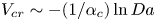 $V_{cr}\sim -({1}/{\alpha _c})\ln Da$. The transition between the two regimes occurs at
 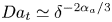 $Da_t\simeq \delta ^{-2\alpha _a/3}$, where
  $\alpha _a=1-\alpha _c$. At
  $\alpha _c=0.5$,
  $Da_t\sim 10$ for
  $\delta =10^{-3}$, and
  $Da_t\sim 10^2$ for
  $\delta =10^{-6}$, showing that the effects of the B–V kinetics on the electroconvective instability become even more important in real electrohydrodynamic systems. For a typical aqueous electrolyte of concentration 0.1 M and
  $\delta =10^{-6}$, the onset voltage for the electroconvective instability almost doubles from
  ${\sim}0.7$ V for
  $Da=10^3$ to
  ${\sim}1.3$V for
  $Da=10^{-2}$. This result can potentially be verified in experiments using electrodes with different ion exchange current density. For instance, in typical salt solutions, the exchange current density is
  $O(1)\ \textrm {A}\ \textrm {cm}^{-2}$ for copper and
  $O(10^{-5})\ \textrm {A}\ \textrm {cm}^{-2}$ for Cobalt (Bockris & Reddy Reference Bockris and Reddy1998). A noticeable difference in the critical voltage for the onset of electroconvection can be expected for these systems. In figure 6(
 $b$), the critical voltage
  $V_{cr}$ increases with decreasing Péclet number
  $Pe$ and it scales as
  $V_{cr}\sim Pe^{-1/2}$ for
  $Pe<10^{-2}$. In a typical aqueous electrolyte, for which
  $Pe\sim 0.1$, the effect of the first-kind slip velocity is important and the critical voltage is higher than the
  ${\sim}Pe^{-1/2}$ scaling. It is worth noting that although the modified slip velocity (4.6b) improves the bulk analysis results for the critical voltage, it still predicts an unstable mode at infinitely large wavenumber, which is intrinsically different from the full analysis.

Figure 6. ( $a$) The dependence of the critical voltage
  $V_{cr}$ on the Damköhler number
  $Da$ at
  $Pe=0.5$. (
 $b$) The dependence of the critical voltage
  $V_{cr}$ on the Péclet number
  $Pe$ for
  $\delta =10^{-5}$.
Figure 7 compares the eigenfunctions of the perturbations with  $k=10$ at different
  $Da$ for
  $V=25, \delta =10^{-3}$ and
  $Pe=0.5$. The plots are normalized such that the perturbed ion concentrations have the same peak value. The perturbations are stable for
  $Da=0.01, 0.1$ and 1 and unstable at larger
  $Da$. At
  $Da=10$ and
  $\infty$, the ion concentration has a large perturbation near the surface and it generates a large disturbance to the potential field and a large slip velocity, thereby causing the electroconvective instability. With decreasing
  $Da$, the concentration disturbance moves away from the surface, leading to a weaker potential field and a smaller slip velocity, and therefore the perturbation decays.

Figure 7. Eigenfunctions for perturbed ( $a, b$) ion concentration, (
 $c$) potential and (
 $d$) velocities for the electroconvective instability predicted by the full analysis for
  $V=25, k=10$ and
  $\delta =10^{-3}$.
4.2. Combined electroconvective and morphological instability
To consider the interaction between the electroconvective and morphological instabilities, we derive the eigenfunctions and eigenvalue with  $h=h_1\, \textrm {e}^{\textrm {i}kx+\sigma t}$ being an unknown variable. In the full analysis, the perturbed equations for
  $c_1^\pm, \varPhi _1$ and
  ${\boldsymbol u}_1$ and the boundary conditions at
  $y=1$ are the same as (4.1) and (4.3a–d). The boundary conditions at
  $y=0$ become
 $$\begin{gather} c_1^{-\prime}-c_0^-\varPhi_1'-c_1^-\varPhi_0'=0, \end{gather}$$
 $$\begin{gather}c_1^{+\prime}+c_0^+\varPhi_1'+c_1^+\varPhi_0' =2Da[(c^+_1+c^{+\prime}_0h_1+c^+_0\alpha_cG)\, \textrm{e}^{\alpha_c\varPhi_0} +\alpha_aG\, \textrm{e}^{-\alpha_a\varPhi_0}], \end{gather}$$
 $$\begin{gather}\sigma h_1 =\frac{\nu_m}{2(1-t_c)}(c_1^{+\prime}+c_0^+\varPhi_1'+c_1^+\varPhi_0'), \end{gather}$$
 $$\begin{gather}c_1^{+\prime}-c_1^{-\prime} +(c_0^{+\prime\prime}-c_0^{-\prime\prime})h_1=0, \end{gather}$$
 $$\begin{gather}v_1=\frac{\sigma h_1}{Pe}, \quad v_1'=0, \end{gather}$$
where  $G=\varPhi _1+\varPhi _0'h_1-Cak^2h_1$. In the limit
  $Da\to \infty$, the perturbed B–V kinetic boundary condition reduces to
  $c^+_1+c^{+\prime }_0h_1+c^+_0G=0$ by applying
  $\ln c^+_0+\varPhi _0=0$ at
  $y=0$.
For the bulk analysis, the growth rate of the purely morphological instability ( $v_1=0$) for large wavenumbers (
 $k\gg 1$) is
 \begin{equation} \sigma=\frac{\nu_mk}{1-t_c}\frac{\dfrac{I}{2} \left(\dfrac{2-b\alpha_a}{\alpha_c}A_c+bA_a\right)-c_sCa(A_c+A_a)k^2} {\dfrac{2-b\alpha_a}{\alpha_c}A_c+bA_a+\dfrac{c_s}{Da}k}, \end{equation}
where  $A_c=c_s\alpha _c\, \textrm {e}^{\alpha _c\varPhi _s}$ and
  $A_a=\alpha _a\, \textrm {e}^{-\alpha _a\varPhi _s}$. The constant
  $b$ is 1 and 2 for underlimiting and limiting currents, respectively. The difference is due to the different dominant mechanisms of ion flux near the surface, ambipolar diffusion and migration, in the two current regimes. The current
  $I$ and the interfacial ion concentration and potential
  $c_s, \varPhi _s$ are solved by (3.2), (3.5a) and (3.6a) for any given voltage. The above equation is very similar to the result of Nielsen & Bruus (Reference Nielsen and Bruus2015a), except the second term in the numerator that arises from a small difference in the form of the B–V condition used in two studies. If one neglects the surface tension (
 $Ca=0$), (4.13) recovers the classical result
  $\sigma =({1}/{2(1-t_c)})\nu _mIk$ for
  $Da\to \infty$, while at a finite
  $Da$, the growth rate approaches a constant value
  $\sigma =({\nu _mIDa}/{2(1-t_c)c_s})((({2-b\alpha _a})/{\alpha _c})A_c+bA_a)$ at large
  $k$.
$k$.
Figure 8 shows the dependence of the growth rate on the wavenumber at different Damköhler numbers and two voltages,  $V=2$ and 25. The growth rate of the morphological instability increases with increasing wavenumber
  $k$ until it reaches a peak value and eventually is stabilized by the surface tension. The growth rate of the morphological instability decreases with decreasing
  $Da$. For
  $k\ll 1$, the growth rate reaches a constant value
  $\sigma =\nu _mI/[2(1-t_c)]$. At an underlimiting current, the bulk analysis in general agrees well with the full analysis at large wavenumbers. At an overlimiting current, the bulk analysis overpredicts the wavenumber
  $k_0$ at which the perturbation becomes stable, showing that the non-electroneutrality of the electrolyte in the space charge layer becomes important at high wavenumbers. The wavenumber
  $k_{m, {M}}$ for the fastest growing morphological mode is of order
  $10^2$–
 $10^3$, representing ramified dendrite growth of the electrodeposition. At a high voltage
  $V=25$, the onset of the electroconvective instability generates a second peak at
  $k_{m, {EC}}\sim O(10)$, corresponding to mossy electrodeposition. Different from our recent work (Li et al. Reference Li, Townsend, Archer and Koch2021), where an imposed shear flow only suppresses the electroconvective instability while not the morphological instability, here decreasing the reaction rate of the surface stabilizes both instabilities. The two peaks of growth rate suggest that the electrodeposition can show very different length scales with and without electroconvection, consistent with previous experiments (Tu et al. Reference Tu, Chao, Sang, Huang and Zou2008; Wei et al. Reference Wei, Cheng, Nath, Tikekar, Li and Archer2018). In the presence of the electroconvection, zinc deposition at the microscopic scale displays an orderly alignment of grain flakes (
 $1\times 2\times 0.1\ \mathrm {\mu }$m) with a preferred orientation, which involves two length scales, the small wavelength (
 $\sim 1\ \mathrm {\mu }$m) determined by an individual grain and the large wavelength (
 $\sim 10^2\ \mathrm {\mu }$m) set by the groups of arrayed grains with the same orientation. When the electroconvection is suppressed by adding agar gel into the electrolyte, the zinc deposition has a morphology of randomly oriented grains which only has the small wavelength (Tu et al. Reference Tu, Chao, Sang, Huang and Zou2008). More recently, Wei et al. (Reference Wei, Cheng, Nath, Tikekar, Li and Archer2018) showed that sodium deposition on a planar metal electrode surface transitions from mossy mushroom structures (large wavelength) to needle-like structures (small wavelength) as electroconvection is suppressed by adding high-molecular-weight molecules into the electrolyte. Our results predict that similar effects can be achieved by decreasing the reaction rate of the surface.

Figure 8. The growth rate for the full analysis of the combined electroconvective (EC) and morphological instability (lines) and the bulk analysis of the purely morphological instability for  $k\gg 1$ (circles) at different
  $Da$.
$Da$.
Figure 9( $a$) shows the characteristic dependence of the wavenumbers of the unstable modes on the applied voltage. The wavenumbers
  $k_{m, {M}}, k_{m, {EC}}$ represent the most unstable electroconvective and morphological modes, and
  $k_0$ is the critical wavenumber below which the growth rate is positive. The two wavenumbers for the morphological instability increase with increasing
  $V$. The slope of the increment becomes smaller at the limiting current due to the formation of the space charge layer. Above a critical voltage, the electroconvective instability incorporating the growth of the electrode surface starts to emerge and
  $k_{m, {EC}}$ has a non-monotonic dependence on
  $V$. Both the electroconvective and morphological modes become more unstable at higher voltage. Yet the growth rate of the most unstable electroconvective mode increases much faster than the most unstable morphological mode, so that the electroconvective mode quickly dominates the electrodeposition with increasing
  $V$. When plotted as a function of
  $V-\varPhi _s$,
  $k_{m, {EC}}$ and
  $k_0$ are nearly independent of
  $Da$, while
  $k_{m, {M}}$ is strongly affected by
  $Da$. Figure 9(
 $b$) shows the dependence of the wavenumber of the most unstable morphological mode on
  $Da$ at
  $V=25$. Furthermore,
  $k_{m, {M}}=k_0/\sqrt {3}$ at large
  $Da$ and it decreases with decreasing
  $Da$. At the limiting current,
  $k_{m, {M}}\sim \delta ^{-1/3}$ since the stabilizing effect of the surface tension is directly influenced by the cation concentration at the electrode–electrolyte interface. Below the limiting current,
  $k_{m, {M}}$ becomes independent of
  $\delta$ and roughly follows a power law scaling with the reaction rate corresponding to
  $k_{m, {M}}\sim Da^{0.45}$ for this specific case of
  $V=25$. At small enough Damköhler number,
  $Da\ll \, \textrm {e}^{-\alpha _cV}$, the current
  $I\simeq 2Da\, \textrm {e}^{\alpha _cV}$ and
  $k_{m, {M}}=Da^{2/3}\, \textrm {e}^{2\alpha _cV/3}(1+\alpha _c)^{2/3}(2\alpha _c Ca)^{-1/3}$. At small and large
  $Da$, the analytical result agrees with the full analysis although it always overestimates
  $k_{m, {M}}$ at large
  $Da$. At intermediate
  $Da$, where the interaction between the kinetics and transport becomes important, the analysis which assumes a strong effect of the perturbed electric field (Nielsen & Bruus Reference Nielsen and Bruus2015a) predicts a constant
  $k_{m, {M}}$ and is inaccurate.

Figure 9. ( $a$) The dependence of the characteristic wavenumbers of the unstable modes on the applied voltage for (red)
  $Da\to \infty$ and (green)
  $Da=1$,
  $\delta =10^{-3}$ obtained from the full analysis. The wavenumbers
  $k_{m, {EC}}$ and
  $k_{m, {M}}$ correspond to the most unstable electroconvective and morphological modes, and
  $k_0$ is the critical wavenumber above which the modes decay. The circles show the voltages at which the growth rate of the most unstable electroconvective mode exceeds that of the morphological mode. (
 $b$) Dependence of
  $k_{m, {M}}$ on
  $Da$ at
  $V=25$. The thick dashed line is an empirical fit.
5. Nonlinear dynamics of electroconvection
To study the nonlinear dynamics of electroconvection near a surface with B–V kinetics, we numerically solve (2.1) in a two-dimensional rectangular domain using a hybrid spectral-finite-volume method (Druzgalski et al. Reference Druzgalski, Andersen and Mani2013; Li et al. Reference Li, Archer and Koch2019). The domain is periodic in the  $x$-direction, and the electric field is applied along the
  $y$-direction. The Stokes equation is solved in Fourier space along the
  $x$-direction and in physical space in the
  $y$-direction. Following the numerical strategy of Druzgalski (Reference Druzgalski2016), we take advantage of the linearity of the velocity and pressure fields and use an unconventional method to impose the incompressibility condition. Along each line of constant
  $x$, the Fourier transformation of the pressure
  $\hat {p}$ is decomposed into three terms
 \begin{equation} \hat{p}=\hat{p}_0+c_1\hat{p}_1+c_2\hat{p}_2, \end{equation}
where  $\hat {p}_0$ satisfies the Poisson equation
  $({\textrm {d}^2}/{{\textrm {d} y}^2}-k^2)\hat {p}_0=ik\hat {f}_{ex}+({\textrm {d}}/{\textrm {d} y})\hat {f}_{ey}$ with homogeneous boundary conditions
  $\hat {p}_0=0$ at
  $y=0$ and 1,
  $\hat {p}_1$ and
  $\hat {p}_2$ satisfy the Laplace equation
  $({\textrm {d}^2}/{{\textrm {d} y}^2}-k^2)\hat {p}_{1,2}=0$ with inhomogeneous boundary condition on one side,
  $\hat {p}_1|_{y=0}=\hat {p}_2|_{y=1}=1$ and
  $\hat {p}_1|_{y=1}=\hat {p}_2|_{y=0}=0$. The coefficients
  $c_1$ and
  $c_2$ are determined by enforcing the incompressible condition at the two boundaries. The full coupling equations (2.1) are solved using Newton's iteration method (Karatay, Druzgalski & Mani Reference Karatay, Druzgalski and Mani2015). In our simulations, five iterations per time step are usually enough to ensure convergence with relative difference less than
  $10^{-5}$. The computational domain is a rectangular domain of aspect ratio 6, the grid is uniform along the
  $x$-direction and stretched in the
  $y$-direction, the grid size is
  $\Delta x=5.8\times 10^{-3}, \Delta y_{min}=10^{-4}$ and
  $\Delta y_{max}=3.6\times 10^{-2}$, the time step is
  $\Delta t=10^{-6}$. The steady state solution for 1-D ion transport is used as the initial state for the simulations.
To validate our numerical simulations, in figures 10 and 11 we compare the average current  $\langle \bar {I}\rangle$, and the average profiles of cation
  $\langle \bar {c}^+\rangle$ and the kinetic energy
  $\langle \overline {E_k}\rangle$ of the electroconvective flows with previous simulations (Druzgalski et al. Reference Druzgalski, Andersen and Mani2013; Pimenta & Alves Reference Pimenta and Alves2018). The angle brackets and overbar represent the averages over the
  $x$-direction and time, respectively. At
  $V=20$, the traditional equilibrium condition predicts an overlimiting current, while the B–V condition as
  $Da\to \infty$ does not. This result is consistent with linear stability analysis which predicts that the critical voltages for the onset of the electroconvective instability with these boundary conditions are
  $V_{cr}=18.53$ and 22.01, respectively (see Appendix for details). The B–V condition predicts slightly weaker electroconvection than the traditional boundary condition because it generates a smaller electroosmotic slip velocity due to the neglect of the double layer. The simulation results for the equilibrium boundary condition agree well with the previous study (Druzgalski et al. Reference Druzgalski, Andersen and Mani2013) at
  $Da\to \infty$.

Figure 10. Comparison the simulation and experiment results of the time- and  $x$-averaged current density
  $\langle \bar {I}\rangle$ at different voltages and Damköhler numbers.

Figure 11. Distribution of ( $a$) time and
  $x$-averaged cation concentration
  $\langle \overline {c^+}\rangle$ and (
 $b$) mean kinetic energy
  $\langle \overline {E_k}\rangle$ versus wall-normal coordinate
  $y$ at different voltages
  $V=20$ (red),
  $V=40$ (green),
  $V=60$ (blue) and
  $V=80$ (black) for
  $\delta =10^{-3}$. The inset in (
 $a$) is a closer view near
  $y=0$.
At a given applied voltage, the interfacial kinetics strongly affects the ion flux on the ion-selective surface. To quantify this effect, we compare the simulation results with the available experimental data in figure 10. Zhang et al. (Reference Zhang, Warren, Li, Cheng, Han, Zhao, Liu, Deng and Archer2020) used 50 mM zinc sulphate solution as electrolyte, zinc metal covered by a Nafion membrane as anode, zinc metal as cathode, the interelectrode distance is 1 cm, and the limiting current density is around 2  $\mathrm {mA}\ \mathrm {cm}^{-2}$. Rubinstein et al. (Reference Rubinstein, Manukyan, Staicu, Rubinstein, Zaltzman, Lammertink, Mugele and Wessling2008) used 10 mM copper sulphate solution as electrolyte, copper metal as anode, Neosepta CMX membrane as cathode, and the interelectrode distance is 0.5 mm. The limiting current density is not reported, but it is probably higher than the one in Zhang et al. (Reference Zhang, Warren, Li, Cheng, Han, Zhao, Liu, Deng and Archer2020) due to a smaller interelectrode distance. In their sulphate solutions, zinc and copper have similar exchange current densities, 1–3
  $\mathrm {mA}\ \mathrm {cm}^{-2}$ for zinc and copper (Milora et al. Reference Milora, Henrickson and Hahn1973; Guerra et al. Reference Guerra, Kelsall, Bestetti, Dreisinger, Wong, Mitchell and Bizzotto2004). In two experiments, the deposition of zinc and copper ions is stable and uniform so the growth of the anode surface is negligible. The result in Zhang et al. (Reference Zhang, Warren, Li, Cheng, Han, Zhao, Liu, Deng and Archer2020) indicates relatively weak kinetic effects, the estimated
  $Da\sim 0.1 - 1$ is consistent with the measurements of the exchange current density. In comparison, the result of Rubinstein et al. (Reference Rubinstein, Manukyan, Staicu, Rubinstein, Zaltzman, Lammertink, Mugele and Wessling2008) indicates a smaller
  $Da$ (
 $\sim 0.01 - 0.1$), the slopes of ohmic and overlimiting currents are smaller, and the onset of overlimiting current occurs at a higher voltage. This difference is highly likely due to the surface kinetics. Indeed, decrease
  $Da$ in simulation improves the comparison with the result of Rubinstein et al. (Reference Rubinstein, Manukyan, Staicu, Rubinstein, Zaltzman, Lammertink, Mugele and Wessling2008).
Figure 12( $a$) shows the time histories of
  $\langle I\rangle$ at different
  $Da$ and
  $V=40$. Decreasing
  $Da$ delays the onset of electroconvection and drastically changes the time history of the current, which successively shows high-frequency oscillation, low-frequency oscillation and a steady state. As expected, the current
  $\langle \bar {I}\rangle$, averaged over time and
  $x$, in general decreases with decreasing
  $Da$, while its variation strongly depends on
  $Da$ (figure 12
 $b$). For
  $Da>10^2$, the overlimiting current is almost independent of
  $Da$ since the interfacial kinetics are fast. From
  $Da=10^2$ to
  $Da=10$,
  $\langle \bar {I}\rangle$ drops significantly from 5.25 to 3.79 because the kinetics limit episodes of high local current density, which can greatly exceed the median current density. For
  $0.1< Da<10$, the average current has a weak dependence on
  $Da$ and a non-monotonic behaviour occurs at
  $Da\sim 0.1$ due to the change of the pattern of the electroconvection. For
  $Da<0.1$,
  $\langle \bar {I}\rangle$ continues to decrease with decreasing
  $Da$ and it eventually reaches the limiting current for
  $Da<10^{-3}$. It is worth noting that the domain size of the numerical simulation affects the overlimiting current and electroconvection. However, its effect becomes less important in the chaotic regime of electroconvection at high voltages and the general trend of current with respect to
  $Da$ is similar for different domain sizes. Perhaps surprisingly, the average interfacial potential
  $\langle \bar {\varPhi }_s\rangle$ is the same as the potential for 1-D ion transport and monotonically increases with decreasing
  $Da$.
$Da$.

Figure 12. ( $a$) Time history of the
  $x$-average current
  $\langle I\rangle$ at
  $V=40$ and
  $\delta =10^{-3}$. Circles show the time instants for the flow fields in figure 13. (
 $b$) The dependence of average current
  $\langle \bar {I}\rangle$ and average interfacial potential
  $\langle \bar {\varPhi }_s\rangle$ on
  $Da$. The red triangles represent the interfacial potential for the 1-D ion transport. The bars show the standard deviations.
The effect of  $Da$ on the current is directly related to the variation of the flow field. Figure 13 shows the typical ion concentration and normal velocity fields at different
  $Da$. The white contour lines show the regions of high cation flux
  $I_y^+=2(1-t_c)Pe\,c^+v-({\partial c^+}/{\partial y}+c^+({\partial \phi }/{\partial y}))=-6$ for figure 13(
 $a$–
$a$– $d$) and
  $I_y^+=-3$ for figure 13(
 $e$). The black lines are the streamlines. For all the cases, the electroconvective vortices inside the gap generate local regions of strong downward flows, which bring more ions from the top to bottom surface and increase the local ion flux (white contour lines). As
  $Da\to \infty$, the flow is composed of large and small vortices, whose sizes correspond to the gap distance (
 ${\sim}1$) and the space charge layer thickness (
 $\delta _s\sim (3V\delta /4)^{2/3}\simeq 0.1$), respectively. The small vortices evolve much faster than the large vortices and generate the high frequency oscillations in the current. At
  $Da=1$, the distinction between the large and small vortices becomes less obvious and the strong interaction between the vortices generates the high frequency fluctuations in the current. Note that the magnitude of the fluid velocity at
  $Da=1$ is slightly larger than the field for
  $Da\to \infty$, meaning that the ion transport is more influenced by the pattern of the electroconvection than by its strength. At
  $Da=0.1$, the flow field has fewer vortices and their interactions become milder. Occasionally, the vortices become very long and induce a weak downward flow and therefore generate a low current (see figure 13
 $d$). At
  $Da=2.5\times 10^{-3}$, the electroconvection has a small velocity and becomes steady. These results are similar to the different flow regimes observed in previous studies with equilibrium boundary conditions by changing the applied voltage (Demekhin et al. Reference Demekhin, Nikitin and Shelistov2013; Druzgalski Reference Druzgalski2016). Here, we show that the transitions can also occur by changing the interfacial kinetics.

Figure 13. The typical concentration and velocity fields (left – cation concentration  $c^+$; right – normal velocity
  $v$) at
  $V=40$ and different
  $Da$. The white contour lines show high flux regions of (
 $a$–
$a$– $d$)
$d$)  $I^+_y=-6$ and (
 $e$)
$e$)  $I^+_y=-3$. The black lines are the streamlines. Movies are available in the supplementary movies are available at https://doi.org/10.1017/jfm.2021.907.
Since the average interfacial potential  $\langle \bar {\varPhi }_s\rangle$ for electroconvection is close to the potential for the 1-D transport problem, it is convenient to characterize the properties of electroconvection as a function of
  $V-\langle \bar {\varPhi }_s\rangle$, and the results are summarized in figure 14. Despite there being scattering, the general trend of the data is clear. The average current increases with increasing potential and it roughly scales as
  $\Delta I\sim \Delta V^{1/2}$, where
  $\Delta I=\langle \bar {I}\rangle -I_{lim}$ is the current increment above the limiting current
  $I_{lim}\simeq 2$ and
  $\Delta V=V-\langle \bar {\varPhi }_s\rangle -(V_{cr}-\langle \bar {\varPhi }_{s, cr}\rangle )$ is the potential increment above the critical voltage difference
  $V_{cr}-\langle \bar {\varPhi }_{s, cr}\rangle \simeq 17$ (see figure 5
 $b$ and 14
 $a$). This scaling can be understood in the following manner. The strength of the electroconvection linearly increases with the voltage difference as confirmed in figure 14(
 $b$), meaning that the Péclet number defined by the characteristic fluid velocity
  $Pe_u=u_cL/D$ linearly increases with
  $V-\langle \bar {\varPhi }_s\rangle$. The classical theory for mass transport due to convection and diffusion with
  $Pe_u\gg 1$ and
  $Re\ll 1$ predicts that the flux scales as
  $\sim Pe_u^{1/2}$ when the normal velocity
  $v\sim y$ such as near a fluid–fluid interface, and
  $\sim Pe_u^{1/3}$ when
  $v\sim y^2$ such as near a no-slip surface (Leal Reference Leal2007). Inside the space charge layer, the cation flux is dominated by the migration so the classical theory for the transport near a no-slip surface is not valid. Instead, we should consider the cation flux at the outer edge of the space charge layer, where the combined contribution of the convective and diffusive fluxes equals the migration flux and accounts for half of the total cation transport. Since the normal velocity grows linearly with the distance away from the edge of the space charge layer and its magnitude increases linearly with the voltage, the increment of ion flux scales as
  $\Delta I\sim \Delta V^{1/2}$. Figure 14(
 $c$) shows the
  $y$-positions of the peak r.m.s. velocities. The peak position for
  $u_{rms}$, which we denote as
  $\delta _x$, can be considered as the thickness of the space charge layer. It roughly remains a constant
  $\delta _x\simeq 0.04$ at all voltages. This value is also close to the position of the maximum value of the average charge density
  $\delta _s$. The thickness of the space charge layer in an electroconvective flow is much smaller than in the 1-D transport problem because the electroconvection mixes the ions and attenuates the ion polarization. The peak position of
  $v_{rms}$, denoted as
  $\delta _y$, increases with increasing potential difference, showing that the downward and upward flows have longer penetration length into the bulk region at higher voltage. In figure 14(
 $d$), the interfacial cation concentration
  $\langle \bar {c}^+\rangle$ becomes higher than the one in 1-D transport for
  $V-\langle \bar {\varPhi }_s\rangle \gtrsim 17$ because the onset of electroconvection brings more ions to the bottom surface. It increases with the voltage difference and quickly reaches a plateau after
  $V-\langle \bar {\varPhi }_s\rangle \sim 24$, meaning that convection-induced ion accumulation close to the surface is saturated.

Figure 14. The dependence of ( $a$) the average current
  $\langle \bar {I}\rangle$, (
 $b$) the peak values
  $u_{max}$ and
  $v_{max}$ of the root mean square (r.m.s.) of velocities
  $u'$ and
  $v'$, (
 $c$) the corresponding positions
  $\delta _x$ and
  $\delta _y$ for the peaks of
  $u_{max}$ and
  $v_{max}$ and (
 $d$) the average interfacial cation concentration
  $\langle \bar {c}^+_s\rangle$ on
  $V-\langle \bar {\varPhi }_s\rangle$ for simulations with different choices of applied voltage
  $V$ and domain length
  $W$. Fitting curves are plotted to guide the eye. The bars in (
 $a$) and (
 $d$) show the standard deviations. The inset in (
 $a$) shows the scaling of the overlimiting current increment
  $\Delta I=\langle \bar {I}\rangle -I_{lim}$ versus the voltage difference
  $\Delta V=V-\langle \bar {\varPhi }_s\rangle -(V_{cr}-\langle \bar {\varPhi }_{s, cr}\rangle )$. The inset in (
 $b$) shows the definitions of
  $u_{max}, v_{max}$ and
  $\delta _x, \delta _y$ and the distribution of r.m.s. of velocities
  $u'$ and
  $v'$ at
  $V=40$ and
  $Da=1$.
So far we have shown that the Damköhler number  $Da$ affects electroconvection mainly by changing the average interfacial potential
  $\langle \bar {\varPhi }_s\rangle$, which is close to the potential for 1-D transport. The potential difference
  $V-\langle \bar {\varPhi }_s\rangle$ across the electrolyte can well describe the properties of electroconvection averaged in time and spanwise direction. To capture the entire picture of the effects of interfacial kinetics, however, we also look into the non-averaged properties. Figure 15 compares the instantaneous distributions of several different variables across the electrolyte along the
  $x$-axis for
  $Da=200, 20$ and 2 at
  $t=1.6$ and
  $V=40$. In all three cases, the downward flow increases the local interfacial cation concentration (green lines) and enhances the local cation transport (blue lines). However, the distributions of the electric potential are different. The downward flow decreases the local interfacial potential
  $\varPhi _s$ at
  $Da=200$, while it increases
  $\varPhi _s$ at
  $Da=20$ and 2 (red lines). At large
  $Da$,
$Da$,  $\varPhi _s$ decreases in the region of downward flow because the local cation concentration increases while retaining a constant chemical potential
  $\ln c_s+\varPhi _s=0$ at the electrode–electrolyte interface. However, the cations brought by the flow are not consumed rapidly at small
  $Da$ and their accumulation at the interface increases the local potential. This effect is directly related to
  $Da$ instead of
  $V-\langle \bar {\varPhi }_s\rangle$ and significantly affects the cation transport inside the electrolyte–electrode interface (thick black lines). At
  $Da=200$, the migration of cations counteracts the diffusion and the flux inside the interface
  $I_x^+$ is negligible. In comparison, at
  $Da=20$ and 2, both migration and diffusion drive the cations away from the local influx region and have a stabilizing effect on the ion deposition on the interface. Since the morphological stability of the ion-depositing surface is largely influenced by the cation distribution on the surface, this effect can potentially be utilized to achieve uniform ion deposition.

Figure 15. The instantaneous distribution of different variables across the electrolyte along the  $x$-axis for (
 $a$)
$a$)  $Da=200$ (
 $b$)
$b$)  $Da=20$ and (
 $c$)
$c$)  $Da=2$ at
  $t=1.6$,
  $V=40$. The grey regions show the normal velocity
  $v$ of the fluid. The alternating regions of positive and negative
  $v$ show the upward and downward flows at this particular time instant. The red solid and green dash–dotted lines show the fluctuations of the interfacial potential
  $\varPhi _s-\langle \bar {\varPhi }_s\rangle$ and the interfacial cation concentration
  $c_s-\langle \bar {c}_s\rangle$, the average potentials are
  $\langle \bar {\varPhi }_s\rangle =5.19, 6.69, 10.5$ and concentration
  $\langle \bar {c}_s\rangle =8.7\times 10^{-3}, 7.8\times 10^{-3}, 7.9\times 10^{-3}$, respectively. The thick black and blue dotted lines show the two components of the cation flux
  $I_x^+$ and
  $I_y^+$ at the bottom surface.
6. Conclusion
To summarize, we investigate the effects of the interfacial kinetics on the linear instability and nonlinear electrohydrodynamics of ion transport in a liquid electrolyte. In the linear stability analysis, we consider both the electroconvective instability near a fixed ion-selective surface and the morphological instability of electrodeposition. For the nonlinear dynamics, the electroconvection near the ion-selective surface is simulated in a two-dimensional domain using a hybrid spectral-finite-volume method. The ion transport, the electric field and the fluid flow are modelled by solving the Nernst–Planck–Poisson–Stokes equations. The kinetics of the cations on the electrode–electrolyte interface are modelled using the B–V equation with the key dimensionless parameter, the Damköhler number  $Da$, and a gradient condition for the cation concentration is used to describe the boundary condition at the inner edge of the space charge layer. This treatment avoids resolving the double layer and predicts very similar results as the traditional equilibrium condition for the 1-D ion transport as
  $Da\to \infty$.
Our study shows that finite reaction rates significantly affect the ion transport in many ways. Decreasing  $Da$ reduces the 1-D transport, increases the critical voltage for the onset of the electroconvective instability, decreases the growth rate of the morphological instability, and changes the patterns of the electroconvective flows and the overlimiting current. For the electroconvective instability, we derive an analytical prediction for the critical voltage using the bulk analysis in (4.8). It extends Rubinstein's results for the critical voltage of infinite interfacial kinetics rate (Rubinstein et al. Reference Rubinstein, Zaltzman and Lerman2005) to arbitrary
  $Da$ and agrees well with the result of the full analysis. We find that the critical voltage for the onset of the electroconvective instability is
  $V_{cr}\simeq V^*_{cr}-\frac {4}{3}\ln \delta$ for
  $Da>\delta ^{-2\alpha _a/3}$, where the bulk analysis prediction
  $V^*_{cr}$ only depends on the Péclet number
  $Pe$ and the transference number of the cation, and
  $\frac {4}{3}\ln \delta$ is the voltage difference across the double layer and the space charge layer. This result is consistent with the previous analysis of
  $Da\to \infty$ (Zaltzman & Rubinstein Reference Zaltzman and Rubinstein2007). At smaller
  $Da$, the critical voltage increases with decreasing
  $Da$ and scales as
  $V_{cr}\simeq V^*_{cr}-({1}/{\alpha _c})\ln Da$. By introducing the interfacial potential
  $\varPhi _s$, we find that the 1-D transport and the electroconvective instability are simply determined by the effective voltage
  $V_e=V-\varPhi _s$ across the liquid electrolyte regardless of the total voltage. These results are helpful to understand the electroconvection near a metal surface with stable electrodeposition. Future experiments can directly test our prediction by measuring the voltage difference across the liquid electrolyte. For the morphological instability, our results show that the bulk analysis (Nielsen & Bruus Reference Nielsen and Bruus2015a) agrees reasonably well with the full analysis result for
  $Da\ll 1$ and
  $Da\gg 1$, whereas for
  $Da\sim 1$ which is more common in real applications, it largely overestimates the wavenumber of the most unstable mode. The growth rate approaches a constant value
  $\sigma \sim Da$ at finite
  $Da$ whereas
  $\sigma \sim k$ for
  $Da\to \infty$. At large
  $k$, the morphological instability is suppressed by the surface tension above a wavenumber that is solely determined by
  $V_e$. In contrast, the wavenumber for the most unstable morphological mode depends on
  $Da$ and
  $V_e$. These results can be applied to guide the design of electrochemical cells. For example, one can modify the exchange current density by coating a polymer layer on the electrode to reduce the morphological instability (Lopez et al. Reference Lopez, Pei, Oh, Wang, Cui and Bao2018).
Above the critical voltage for the onset of the electroconvective instability, numerical simulation shows that decreasing  $Da$ attenuates the strength of electroconvection. The average interfacial potential
  $\langle \bar {\varPhi }_s\rangle$ in the presence of nonlinear electroconvection is the same as the potential
  $\varPhi _s$ in 1-D transport. The voltage across the liquid electrolyte
 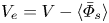 $V_e=V-\langle \bar {\varPhi }_s\rangle$ largely determines the transitions between different modes of electroconvection as well as the key properties of the flows. With increasing
  $V_e$, the electroconvection transits from steady vortices to unsteady flow composed of large vortices with relatively weak interactions, and eventually becomes a chaotic flow with vortices of different sizes that interact strongly. The common feature of the vortices is that they generate downward flow which increases the local cation concentration and generates local high-current hot spots. The strength of the electroconvection roughly follows a linear relation with
  $V_e$. The average overlimiting current scales as
 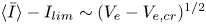 $\langle \bar {I}\rangle -I_{lim}\sim (V_e-V_{e,cr})^{1/2}$ due to the existence of the space charge layer. This result is similar to the mass transport near a fluid interface for
  $Re\ll 1$ and
  $Pe\gg 1$.
The interfacial kinetics have a strong influence on the ion diffusion inside the electrolyte–electrode interface. While the local hot spots always increase the local interfacial cation concentration  $c^+_s$, their effects on the interfacial potential
  $\varPhi _s$ depend on the Damköhler number. At large
  $Da$,
$Da$,  $\varPhi _s$ is lower in the hot spot regions than the surroundings. At small
  $Da$, the result is the opposite, meaning that both diffusion and migration drive the cations away from the hot spots and therefore weaken the morphological instability. This effect can only be observed near an interface with finite kinetic rates. Although in the current study the lateral transport of ions inside the interface is two orders of magnitude smaller than the transport in the normal direction, we expect that this effect may be more dramatic in a highly conducting interfacial layer, such as the sodium bromide interphase layer (Choudhury et al. Reference Choudhury2017), so that is may help to mitigate the dendritic electrodeposition. Finally, it would be of interest to determine how the insights obtained in the present study into the effects of surface kinetics on electroconvection influence the unstable electrodeposition on a metal surface, without accounting for the nonlinear evolution of electrode surface. The coupling between deposition and convection near an electrode surface with nonlinear morphological evolution has important implications in diverse applications and should be rigorously investigated in future studies.
Supplementary movies
Supplementary movies are available at https://doi.org/10.1017/jfm.2021.907.
Funding
This work was supported by Department of Energy Basic Energy Science grant DE-SC0016082. G.L. thanks to the Natural Science Foundation of China (Grant 1210021309). The work of A.T. is supported by NSF-DMS grant 1818757.
Declaration of interests
The authors report no conflict of interest.
Appendix. Electroconvective instability with different boundary conditions
We compare the electroconvective instability using two different boundary conditions, the traditional equilibrium boundary condition applied inside a resolved double layer, and the new condition (2.2)–(2.6) at  $Da\to \infty$ applied without resoling the double layer. Figure 16 shows the neutral stability curves for the two conditions at different double layer thickness. The new condition predicts a higher critical voltage for the onset of electroconvection than the traditional condition by a constant voltage. The comparison of the eigenfunctions in figure 17 shows that the difference between the two results is mainly caused by the perturbed electric potential field. The new condition predicts a smaller potential inside the space charge layer and therefore leads to a weaker electroosmotic flow.

Figure 16. Comparison of the neutral curves for the electroconvective instability derived by two different boundary conditions. In ( $b$), the lines for the traditional boundary conditions which resolve the double layer are shifted upward by a constant voltage
 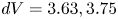 $dV=3.63, 3.75$ and 3.89 for
  $\delta =10^{-3}, 10^{-4}$ and
  $10^{-5}$, respectively.

Figure 17. Comparison of the eigenfunctions for the electroconvective instability using two different boundary conditions for  $V=40, k=10$ and
  $\delta =10^{-3}$.


